Lévy-stable two-pion Bose-Einstein correlations in √
s
NN= 200 GeV Au + Au collisions
A. Adare,12C. Aidala,39,45N. N. Ajitanand,63,*Y. Akiba,57,58,†R. Akimoto,11J. Alexander,63M. Alfred,24H. Al-Ta’ani,52 A. Angerami,13K. Aoki,32,57N. Apadula,29,64Y. Aramaki,11,57H. Asano,35,57E. C. Aschenauer,7E. T. Atomssa,64 T. C. Awes,54B. Azmoun,7V. Babintsev,25A. Bagoly,17M. Bai,6B. Bannier,64K. N. Barish,8B. Bassalleck,51S. Bathe,5,58
V. Baublis,56S. Baumgart,57A. Bazilevsky,7R. Belmont,12,69A. Berdnikov,60Y. Berdnikov,60D. S. Blau,34,50M. Boer,39 J. S. Bok,51,52,72K. Boyle,58M. L. Brooks,39J. Bryslawskyj,5,8H. Buesching,7V. Bumazhnov,25S. Butsyk,51S. Campbell,13,64
V. Canoa Roman,64P. Castera,64C.-H. Chen,58,64C. Y. Chi,13M. Chiu,7I. J. Choi,26J. B. Choi,10,*S. Choi,62 R. K. Choudhury,4P. Christiansen,41T. Chujo,68O. Chvala,8V. Cianciolo,54Z. Citron,64,70B. A. Cole,13M. Connors,21,58,64
M. Csanád,17T. Csörgő,18,71S. Dairaku,35,57T. W. Danley,53A. Datta,44M. S. Daugherity,1G. David,7,64K. DeBlasio,51 K. Dehmelt,64A. Denisov,25A. Deshpande,58,64E. J. Desmond,7K. V. Dharmawardane,52O. Dietzsch,61L. Ding,29
A. Dion,29,64J. H. Do,72M. Donadelli,61L. D’Orazio,43O. Drapier,36A. Drees,64K. A. Drees,6J. M. Durham,39,64 A. Durum,25S. Edwards,6Y. V. Efremenko,54T. Engelmore,13A. Enokizono,54,57,59S. Esumi,68K. O. Eyser,7,8B. Fadem,46
W. Fan,64N. Feege,64D. E. Fields,51M. Finger,9M. Finger, Jr.,9F. Fleuret,36S. L. Fokin,34J. E. Frantz,53A. Franz,7 A. D. Frawley,20Y. Fukao,57Y. Fukuda,68T. Fusayasu,48K. Gainey,1C. Gal,64P. Gallus,14P. Garg,3,64A. Garishvili,66 I. Garishvili,38H. Ge,64A. Glenn,38X. Gong,63M. Gonin,36Y. Goto,57,58R. Granier de Cassagnac,36N. Grau,2S. V. Greene,69
M. Grosse Perdekamp,26T. Gunji,11L. Guo,39H.- ˚A. Gustafsson,41,*T. Hachiya,57,58J. S. Haggerty,7K. I. Hahn,19 H. Hamagaki,11S. Y. Han,19J. Hanks,13,64S. Hasegawa,30T. O. S. Haseler,21K. Hashimoto,57,59E. Haslum,41R. Hayano,11
X. He,21T. K. Hemmick,64T. Hester,8J. C. Hill,29K. Hill,12A. Hodges,21R. S. Hollis,8K. Homma,23B. Hong,33 T. Horaguchi,68Y. Hori,11T. Hoshino,23N. Hotvedt,29J. Huang,7S. Huang,69T. Ichihara,57,58H. Iinuma,32Y. Ikeda,57,68 J. Imrek,16M. Inaba,68A. Iordanova,8D. Isenhower,1M. Issah,69D. Ivanishchev,56B. V. Jacak,64M. Javani,21Z. Ji,64J. Jia,7,63
X. Jiang,39B. M. Johnson,7,21K. S. Joo,47V. Jorjadze,64D. Jouan,55D. S. Jumper,26J. Kamin,64S. Kaneti,64B. H. Kang,22 J. H. Kang,72J. S. Kang,22J. Kapustinsky,39K. Karatsu,35,57S. Karthas,64M. Kasai,57,59G. Kasza,17,18D. Kawall,44,58 A. V. Kazantsev,34T. Kempel,29V. Khachatryan,64A. Khanzadeev,56K. M. Kijima,23B. I. Kim,33C. Kim,8,33D. J. Kim,31 E.-J. Kim,10H. J. Kim,72K.-B. Kim,10M. Kim,62M. H. Kim,33Y.-J. Kim,26Y. K. Kim,22D. Kincses,17E. Kinney,12Á. Kiss,17 E. Kistenev,7J. Klatsky,20D. Kleinjan,8P. Kline,64T. Koblesky,12Y. Komatsu,11,32B. Komkov,56J. Koster,26D. Kotchetkov,53
D. Kotov,56,60A. Král,14F. Krizek,31S. Kudo,68G. J. Kunde,39B. Kurgyis,17K. Kurita,57,59M. Kurosawa,57,58Y. Kwon,72 G. S. Kyle,52R. Lacey,63Y. S. Lai,13J. G. Lajoie,29A. Lebedev,29B. Lee,22D. M. Lee,39J. Lee,19,65K. B. Lee,33K. S. Lee,33
S. H. Lee,29,64S. R. Lee,10M. J. Leitch,39M. A. L. Leite,61M. Leitgab,26Y. H. Leung,64B. Lewis,64N. A. Lewis,45X. Li,39 S. H. Lim,39,72L. A. Linden Levy,12M. X. Liu,39S. Lökös,17,18B. Love,69D. Lynch,7C. F. Maguire,69Y. I. Makdisi,6
M. Makek,70,73A. Manion,64V. I. Manko,34E. Mannel,7,13H. Masuda,59S. Masumoto,11,32M. McCumber,12,39 P. L. McGaughey,39D. McGlinchey,12,20,39C. McKinney,26M. Mendoza,8B. Meredith,26W. J. Metzger,18Y. Miake,68 T. Mibe,32A. C. Mignerey,43D. E. Mihalik,64A. Milov,70D. K. Mishra,4J. T. Mitchell,7G. Mitsuka,58Y. Miyachi,57,67
S. Miyasaka,57,67A. K. Mohanty,4S. Mohapatra,63H. J. Moon,47T. Moon,72D. P. Morrison,7S. I. Morrow,69
S. Motschwiller,46T. V. Moukhanova,34T. Murakami,35,57J. Murata,57,59A. Mwai,63T. Nagae,35K. Nagai,67S. Nagamiya,32,57 K. Nagashima,23J. L. Nagle,12M. I. Nagy,17,71I. Nakagawa,57,58H. Nakagomi,57,68Y. Nakamiya,23K. R. Nakamura,35,57 T. Nakamura,57K. Nakano,57,67C. Nattrass,66A. Nederlof,46M. Nihashi,23,57R. Nouicer,7,58T. Novák,18,71N. Novitzky,31,64
A. S. Nyanin,34E. O’Brien,7C. A. Ogilvie,29K. Okada,58J. D. Orjuela Koop,12J. D. Osborn,45A. Oskarsson,41 M. Ouchida,23,57K. Ozawa,11,32,68R. Pak,7V. Pantuev,27V. Papavassiliou,52B. H. Park,22I. H. Park,19,65J. S. Park,62
S. Park,57,62,64S. K. Park,33S. F. Pate,52L. Patel,21M. Patel,29H. Pei,29J.-C. Peng,26W. Peng,69H. Pereira,15 D. V. Perepelitsa,7,12,13G. D. N. Perera,52D.Yu. Peressounko,34C. E. PerezLara,64R. Petti,7,64C. Pinkenburg,7R. P. Pisani,7 M. Proissl,64A. Pun,53M. L. Purschke,7H. Qu,1P. V. Radzevich,60J. Rak,31I. Ravinovich,70K. F. Read,54,66D. Reynolds,63 V. Riabov,50,56Y. Riabov,56,60E. Richardson,43D. Richford,5T. Rinn,29D. Roach,69G. Roche,40,*S. D. Rolnick,8M. Rosati,29
Z. Rowan,5J. Runchey,29B. Sahlmueller,64N. Saito,32T. Sakaguchi,7H. Sako,30V. Samsonov,50,56M. Sano,68M. Sarsour,21 K. Sato,68S. Sato,30S. Sawada,32B. K. Schmoll,66K. Sedgwick,8R. Seidl,57,58A. Sen,21,29,66R. Seto,8A. Sexton,43 D. Sharma,64,70I. Shein,25T.-A. Shibata,57,67K. Shigaki,23M. Shimomura,29,49,68K. Shoji,35,57P. Shukla,4A. Sickles,7,26
C. L. Silva,29,39D. Silvermyr,41,54K. S. Sim,33B. K. Singh,3C. P. Singh,3V. Singh,3M. J. Skoby,45M. Slunečka,9 R. A. Soltz,38W. E. Sondheim,39S. P. Sorensen,66I. V. Sourikova,7P. W. Stankus,54E. Stenlund,41M. Stepanov,44,*A. Ster,71
S. P. Stoll,7T. Sugitate,23A. Sukhanov,7J. Sun,64J. Sziklai,71E. M. Takagui,61A. Takahara,11A Takeda,49A. Taketani,57,58 Y. Tanaka,48S. Taneja,64K. Tanida,30,58,62M. J. Tannenbaum,7S. Tarafdar,3,69A. Taranenko,50,63G. Tarnai,16E. Tennant,52 H. Themann,64R. Tieulent,42A. Timilsina,29T. Todoroki,57,68L. Tomášek,28M. Tomášek,14,28H. Torii,23C. L. Towell,1 R. S. Towell,1I. Tserruya,70Y. Tsuchimoto,11T. Tsuji,11Y. Ueda,23B. Ujvari,16C. Vale,7H. W. van Hecke,39M. Vargyas,17,71 S. Vazquez-Carson,12E. Vazquez-Zambrano,13A. Veicht,13J. Velkovska,69R. Vértesi,71M. Virius,14A. Vossen,26V. Vrba,14,28 E. Vznuzdaev,56X. R. Wang,52,58Z. Wang,5D. Watanabe,23K. Watanabe,68Y. Watanabe,57,58Y. S. Watanabe,11F. Wei,29,52
R. Wei,63S. N. White,7D. Winter,13S. Wolin,26C. L. Woody,7M. Wysocki,12,54B. Xia,53C. Xu,52Q. Xu,69
Y. L. Yamaguchi,11,57,58,64R. Yang,26A. Yanovich,25P. Yin,12J. Ying,21S. Yokkaichi,57,58J. H. Yoo,33Z. You,39I. Younus,37,51 H. Yu,52I. E. Yushmanov,34W. A. Zajc,13A. Zelenski,6S. Zharko,60and L. Zou8
(PHENIX Collaboration)
1Abilene Christian University, Abilene, Texas 79699, USA
2Department of Physics, Augustana University, Sioux Falls, South Dakota 57197, USA
3Department of Physics, Banaras Hindu University, Varanasi 221005, India
4Bhabha Atomic Research Centre, Bombay 400 085, India
5Baruch College, City University of New York, New York, New York 10010, USA
6Collider-Accelerator Department, Brookhaven National Laboratory, Upton, New York 11973-5000, USA
7Physics Department, Brookhaven National Laboratory, Upton, New York 11973-5000, USA
8University of California-Riverside, Riverside, California 92521, USA
9Charles University, Ovocný trh 5, Praha 1, 116 36, Prague, Czech Republic
10Chonbuk National University, Jeonju, 561-756, Korea
11Center for Nuclear Study, Graduate School of Science, University of Tokyo, 7-3-1 Hongo, Bunkyo, Tokyo 113-0033, Japan
12University of Colorado, Boulder, Colorado 80309, USA
13Columbia University, New York, New York 10027 and Nevis Laboratories, Irvington, New York 10533, USA
14Czech Technical University, Zikova 4, 166 36 Prague 6, Czech Republic
15Dapnia, CEA Saclay, F-91191, Gif-sur-Yvette, France
16Debrecen University, H-4010 Debrecen, Egyetem tér 1, Hungary
17ELTE, Eötvös Loránd University, H-1117 Budapest, Pázmány P.s. 1/A, Hungary
18Eszterházy Károly University, Károly Róbert Campus, H-3200 Gyöngyös, Mátrai út 36, Hungary
19Ewha Womans University, Seoul 120-750, Korea
20Florida State University, Tallahassee, Florida 32306, USA
21Georgia State University, Atlanta, Georgia 30303, USA
22Hanyang University, Seoul 133-792, Korea
23Hiroshima University, Kagamiyama, Higashi-Hiroshima 739-8526, Japan
24Department of Physics and Astronomy, Howard University, Washington, DC 20059, USA
25IHEP Protvino, State Research Center of Russian Federation, Institute for High Energy Physics, Protvino, 142281, Russia
26University of Illinois at Urbana-Champaign, Urbana, Illinois 61801, USA
27Institute for Nuclear Research of the Russian Academy of Sciences, prospekt 60-letiya Oktyabrya 7a, Moscow 117312, Russia
28Institute of Physics, Academy of Sciences of the Czech Republic, Na Slovance 2, 182 21 Prague 8, Czech Republic
29Iowa State University, Ames, Iowa 50011, USA
30Advanced Science Research Center, Japan Atomic Energy Agency, 2-4 Shirakata Shirane, Tokai-mura, Naka-gun, Ibaraki-ken 319-1195, Japan
31Helsinki Institute of Physics and University of Jyväskylä, P.O. Box 35, FI-40014 Jyväskylä, Finland
32KEK, High Energy Accelerator Research Organization, Tsukuba, Ibaraki 305-0801, Japan
33Korea University, Seoul, 136-701, Korea
34National Research Center “Kurchatov Institute,” Moscow 123098, Russia
35Kyoto University, Kyoto 606-8502, Japan
36Laboratoire Leprince-Ringuet, Ecole Polytechnique, CNRS-IN2P3, Route de Saclay, F-91128, Palaiseau, France
37Physics Department, Lahore University of Management Sciences, Lahore 54792, Pakistan
38Lawrence Livermore National Laboratory, Livermore, California 94550, USA
39Los Alamos National Laboratory, Los Alamos, New Mexico 87545, USA
40LPC, Université Blaise Pascal, CNRS-IN2P3, Clermont-Fd, 63177 Aubiere Cedex, France
41Department of Physics, Lund University, Box 118, SE-221 00 Lund, Sweden
42IPNL, CNRS/IN2P3, Université Lyon, Université Lyon 1, F-69622, Villeurbanne, France
43University of Maryland, College Park, Maryland 20742, USA
44Department of Physics, University of Massachusetts, Amherst, Massachusetts 01003-9337, USA
45Department of Physics, University of Michigan, Ann Arbor, Michigan 48109-1040, USA
46Muhlenberg College, Allentown, Pennsylvania 18104-5586, USA
47Myongji University, Yongin, Kyonggido 449-728, Korea
48Nagasaki Institute of Applied Science, Nagasaki-shi, Nagasaki 851-0193, Japan
49Nara Women’s University, Kita-uoya Nishi-machi Nara 630-8506, Japan
50National Research Nuclear University, MEPhI, Moscow Engineering Physics Institute, Moscow, 115409, Russia
51University of New Mexico, Albuquerque, New Mexico 87131, USA
52New Mexico State University, Las Cruces, New Mexico 88003, USA
53Department of Physics and Astronomy, Ohio University, Athens, Ohio 45701, USA
54Oak Ridge National Laboratory, Oak Ridge, Tennessee 37831, USA
55IPN-Orsay, Université Paris-Sud, CNRS/IN2P3, Université Paris-Saclay, BP1, F-91406, Orsay, France
56PNPI, Petersburg Nuclear Physics Institute, Gatchina, Leningrad region, 188300, Russia
57RIKEN Nishina Center for Accelerator-Based Science, Wako, Saitama 351-0198, Japan
58RIKEN BNL Research Center, Brookhaven National Laboratory, Upton, New York 11973-5000, USA
59Physics Department, Rikkyo University, 3-34-1 Nishi-Ikebukuro, Toshima, Tokyo 171-8501, Japan
60Saint Petersburg State Polytechnic University, St. Petersburg 195251, Russia
61Universidade de São Paulo, Instituto de Física, Caixa Postal 66318, São Paulo CEP05315-970, Brazil
62Department of Physics and Astronomy, Seoul National University, Seoul 151-742, Korea
63Chemistry Department, Stony Brook University, SUNY, Stony Brook, New York 11794-3400, USA
64Department of Physics and Astronomy, Stony Brook University, SUNY, Stony Brook, New York 11794-3800, USA
65Sungkyunkwan University, Suwon, 440-746, Korea
66University of Tennessee, Knoxville, Tennessee 37996, USA
67Department of Physics, Tokyo Institute of Technology, Oh-okayama, Meguro, Tokyo 152-8551, Japan
68Tomonaga Center for the History of the Universe, University of Tsukuba, Tsukuba, Ibaraki 305, Japan
69Vanderbilt University, Nashville, Tennessee 37235, USA
70Weizmann Institute, Rehovot 76100, Israel
71Institute for Particle and Nuclear Physics, Wigner Research Centre for Physics, Hungarian Academy of Sciences (Wigner RCP, RMKI) H-1525 Budapest 114, P.O. Box 49, Budapest, Hungary
72Yonsei University, IPAP, Seoul 120-749, Korea
73Department of Physics, Faculty of Science, University of Zagreb, Bijenička c. 32 HR-10002 Zagreb, Croatia
(Received 19 September 2017; published 14 June 2018)
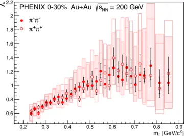
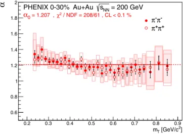
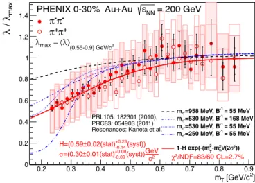
We present a detailed measurement of charged two-pion correlation functions in 0–30% centrality√ sNN = 200 GeV Au+Au collisions by the PHENIX experiment at the Relativistic Heavy Ion Collider. The data are well described by Bose-Einstein correlation functions stemming from Lévy-stable source distributions. Using a fine transverse momentum binning, we extract the correlation strength parameterλ, the Lévy index of stabilityα, and the Lévy length scale parameterRas a function of average transverse mass of the pairmT. We find that the positively and the negatively charged pion pairs yield consistent results, and their correlation functions are represented, within uncertainties, by the same Lévy-stable source functions. Theλ(mT) measurements indicate a decrease of the strength of the correlations at lowmT. The Lévy length scale parameterR(mT) decreases with increasingmT, following a hydrodynamically predicted type of scaling behavior. The values of the Lévy index of stabilityαare found to be significantly lower than the Gaussian case ofα=2, but also significantly larger than the conjectured value that may characterize the critical point of a second-order quark-hadron phase transition.
DOI:10.1103/PhysRevC.97.064911 I. INTRODUCTION
Femtoscopy is a well-established subfield of high-energy particle and nuclear physics that encompasses all the methods that allow for measuring lengths and time intervals on the femtometer (fm) scale. While the name was coined in 2001 [1], several earlier methods were developed in other fields of science that can be considered as predecessors. As femtoscopy typically deals with intensity correlations of particle pairs (or multiplets), the earliest intensity correlation measurements that were performed in radio and optical astronomy to measure the angular diameters of main sequence stars by Hanbury Brown and Twiss (HBT) [2] are considered as the experimental foundations of this field. The clear understanding of the HBT effect, as well as of the lack of intensity correlations in lasers, by Glauber is considered to be the opening of a new and prosperous field of science called quantum optics [3–5].
*Deceased.
†Corresponding author: akiba@rcf.rhic.bnl.gov
Intensity correlations of identical pions were observed in proton-antiproton annihilation while searching for theρmeson [6], and these correlations were explained by Goldhaber, Goldhaber, Lee and Pais (GGLP) on the basis of the Bose- Einstein symmetrization of the wave function of identical pion pairs [7]. Hence, in particle physics these correlations are also called GGLP or simply Bose-Einstein correlations. Because the two-particle Bose-Einstein correlation function is related to the Fourier transform of the phase-space density of the particle emitting source, by measuring the correlation function one can readily map out the particle source on a femtometer scale.
The discovery of the strongly coupled quark gluon plasma (sQGP) at the Relativistic Heavy Ion Collider [8–11] (RHIC) relied also on the contribution from Bose-Einstein correlation studies, beyond other important observables, many of which were confirmed and further elaborated at the Large Hadron Collider (LHC). The approximate transverse mass (mT) de- pendence of the measured Gaussian source radii (RGauss) is R−2Gauss∝a+bmT (where a and b are constants), which is almost universal across collision centrality, particle type, colliding energy, and colliding system size [12,13]. This is a direct consequence of a strong longitudinal as well as radial
hydrodynamical expansion [14–20]. Directional Hubble flows seem to be a crucial property of the sQGP formation in heavy ion collisions, or so-called little bangs [14–17]. The so- called RHIC HBT puzzle, the apparent contradiction between several hydrodynamical model predictions and the observed ratio of the HBT radii [8,9], also turned out to be resolv- able in a hydrodynamical picture with more realistic physics conditions and refined models of three-dimensional Hubble flows [15,18,19,21–23]. For a more detailed introduction and review of Bose-Einstein correlations and their application in high-energy heavy-ion collisions, see the review papers in Refs. [20,24–32].
To fully exploit the power of HBT correlations (as observ- ables deemed to provide insight into the dynamics of the matter produced in heavy-ion collisions), one can and must go beyond the Gaussian parameterization and the Gaussian source radii, as observed ine+e−collisions at the Large Electron-Positron Collider (LEP) [33] and inp+p,p+Pb, and Pb+Pb collisions at the LHC [34–36]. One of the observables that is rather sensitive to the actual shape of the Bose-Einstein correlation function is the so-called “intercept parameter” (or strength)λ of the correlation function, as its value depends on the result of an extrapolation of the observed correlation function to zero relative momentum. The experimental determination of the parameterλfor pions can provide information about the ratio of primordial pions to those that are decay products of long-lived resonances [37,38] and may also give insight into the possibility of coherent pion production [25,27,37]. The shape of the correlation functions, in particular their non-Gaussian behavior, may also hint at the vicinity of the critical point of the quark-hadron phase transition [39,40].
In this paper, we present a precise measurement of two- pion HBT correlation functions in√
sNN =200 GeV Au+Au collisions by the PHENIX experiment at RHIC. We use the data recorded in the 2010 data-collection period. This data sample allows us to use a fine transverse mass binning and to infer the shape of the correlation function more precisely than was possible with earlier data sets. The significance of this will become evident when we extract the source parameters. It turns out that the measured correlation functions cannot be described by a Gaussian approximation in a statistically acceptable way.
A generalized random walk or anomalous diffusion suggests the appearance of Lévy-stable distributions for the phase-space density of the particle emitting source [40,41]. We have inves- tigated whether a Lévy-stable generalization of the Gaussian source distributions is consistent with our measurements and found that (with the proper treatment of the final-state Coulomb interaction) Lévy-stable source distributions—applied here for the first time in heavy-ion HBT analyses—give a high-quality, statistically acceptable description of the measured correlation functions.
The structure of this paper is as follows: SectionIIpresents the PHENIX experimental setup with emphasis on the tracking and particle identification detectors that were used for this analysis. In Sec.III, we present the measurement procedure of the two-pion correlation functions. In Sec.IV, we discuss the shape analysis of the measured HBT correlation functions for Lévy-stable source distributions, and the procedure for determining the Lévy parameters. In Sec.VI, we present our
West Beam View PHENIX Detector 2010
East
HBD
PbSc PbSc
PbSc PbSc
PbSc PbGl
PbSc PbGl
TOF-E
PC1 PC1
PC3 PC2
Central
Magnet TECPC3
BB
RICH RICH
DC DC
Aerogel
TOF-W 7.9 m = 26 ft
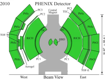
FIG. 1. View of the PHENIX central arm spectrometer detector setup during the 2010 run.
results, namely the extracted Lévy parameters of the source as a function of the transverse mass of the pair. We also discuss here some of the possible interpretations of these results. Finally, we summarize and conclude.
II. EXPERIMENTAL SETUP
The PHENIX experiment was designed to study various different particle types produced in heavy-ion collisions, including photons, electrons, muons, and charged hadrons, trading spatial acceptance for segmentation, good energy and momentum resolution, and high luminosity capability. Figure1 shows a schematic beam view drawing of the PHENIX exper- iment during the 2010 data-collection period. The detailed de- scription of the basic experimental configuration (without the upgrades made after the early 2000s) can be found elsewhere [42]; here we give only a brief description of the detectors that played a role in this analysis.
A. Event characterization detectors
This analysis uses the beam-beam counters (BBC) for event characterization. Its two arms (“north” and “south”) are located at±144 cm along the beam axis (zaxis) from the center of PHENIX, corresponding to the 3.0<|η|<3.9 pseudorapid- ity interval. Each arm of the BBC contains 64 quartzČerenkov counters, covering 2πin azimuth. They provide minimum-bias (MB) triggering; the MB trigger condition requires at least two hits in coincidence in both BBC arms, thus capturing 92±3%
of the total Au+Au inelastic cross section [43]. The charge sum in both BBC arms is used for event centrality determination.
The BBCs also measure the average hit time in the north- and south-arm photomultipliers (PMTs), thus providing collision vertex position measurements along thezdirection (from the hit time difference) as well as initial timing information for the collision. With an intrinsic timing resolution of≈40 ps, thez-vertex resolution is≈0.5 cm and≈1.5 cm in central and peripheral Au+Au collisions, respectively.
B. Central arm tracking
PHENIX has two central arm spectrometers (“east” and
“west”), each covering|η|<0.35 in pseudorapidity andϕ = π/2 in azimuth, as seen in Fig.1. In each central arm, charged particle tracks are reconstructed using hit information from the drift chamber (DC), the first layer of pad chambers (PC1), and the collisionz-vertex position measured by the BBC [44].
The DCs are located at a radial distance of 202–246 cm from the beam axis. They provide trajectory measurement in the transverse plane, with an angular resolution of≈1 mrad. The PC1s are multiwire proportional chambers with pad readout, located immediately behind the DCs. They provide track position measurement both in theϕ andzdirections, with a zresolution of≈1.7 mm.
The PHENIX central arm spectrometer magnet generates a magnetic field approximately parallel to the beam line.
It comprises two pairs of independently operable concen- tric coils, an inner and an outer coil pair, located at radial distances of ≈60 cm and ≈180 cm, respectively. The DCs are positioned so that they are in the reduced field region.
Charged-particle-momentum determination is enabled by the measurement of the bending of the track in the magnetic field.
The transverse momentumpT is determined by the bending angle measured by the DC, while the polar angle of the momentum is determined by the zcoordinate measured by PC1 and thez-vertex coordinate from the BBC. Reconstructed tracks are then projected to the outer detectors used for track verification and timing measurement.
Because at not too low pT the momentum resolution is governed mainly by the angular resolution of the DC, high bending fields are desirable. Thus, usually the two coil pairs are operated with currents flowing in the same direction (this is called “++” or “−−” mode), to achieve the designed maximum total field integral of
Bdl≈1.1 T m (this is the relevant quantity for the bending, and in turn for the momentum measurement).
In 2010, the Hadron Blind Detector (HBD), a specialized Čerenkov counter located around the nominal collision point for the measurement of dielectron pairs, was installed [45].
The operation of the HBD required a fieldfree region around the collision point, which was achieved by running the inner and outer coils in the opposite directions (in “+−” or “−+” modes). This reduced the field integral to≈40% of its maxi- mum value. However, the present analysis deals with low- and intermediate-pT hadrons (up topT ≈0.85 GeV/c), so high- pT momentum resolution is not crucial. (The momentum res- olution forpT in the dataset used is estimated to beδpT/pT ≈ 1.3%⊕1.2%×pT[GeV/c] [46]. Thepzmomentum resolu- tion has, in addition, a component stemming from the BBC z-vertex resolution.) Moreover, the reduced magnetic field had a beneficial side effect for the present analysis. Namely, the low-momentum acceptance of this dataset is extended to lower values of transverse momentum, enabling a relatively clean identified pion sample down topT ≈0.2 GeV/c. This would have been much harder, if not impossible, with the normal++
or−−field setting, because of too large bending angles and residual bending outside of the DC nominal radius, which is not taken into account in the standard PHENIX track projection algorithm.
C. Particle identification detectors
In the present analysis, we identify charged pions by their time of flight from the collision point to the outer detectors. We use the lead-scintillator electromagnetic calorimeter (PbSc) as well as the high-resolution time-of-flight detectors (TOF east and TOF west) [47].
The PbSc is a sampling calorimeter located approximately 5.1 m radial distance from the beam axis. It covers|η|<0.35 in both arms, and in terms ofϕ, it covers allπ/2 acceptance of the west arm, andπ/4 (i.e., half) of the east arm, as seen in Fig.1. It is a finely segmented detector, consisting of 15 552 individual channels (“towers”). After careful tower-by-tower and energy- dependent calibration, a timing resolution of ≈400–600 ps (depending on deposited energy, incident angle, individual channel electronics imperfections, etc.) was achieved for pions.
The part of the east arm acceptance not covered by the PbSc is covered by the lead-glass (PbGl) calorimeter, which has a much worse timing resolution for hadrons and thus was not used for the present analysis.
The TOF east detector is also located at approximately 5.1 m from the beam axis and covers much of the PbGl acceptance in the east arm. It is made of 960 plastic scintillator slats, with two PMTs attached to each side of them. After calibration, the timing resolution was found to be ≈150 ps [48]. The TOF west detector takes advantage of the multigap resistive plate chamber (MRPC) technology. It has two separate panels, each coveringϕ≈π/16 in the west arm, at around 4.8 m radial distance from the beam pipe. Each panel comprises 64 MRPCs and has 256 individual copper readout strips. After calibration, a timing resolution of≈90 ps was achieved.
III. MEASUREMENT OF TWO-PION CORRELATION FUNCTIONS
A. Event and track selection, particle identification The MB-triggered data sample used in this analysis com- prises≈7.3×10⁹√
sNN=200 GeV Au+Au events recorded by PHENIX during the 2010 running period. This sample is reduced to ≈2.2×10⁹ events when we apply a 0–30%
centrality selection. The event z-vertex position was con- strained between±30 cm in order to have an efficient BBC response as well as to avoid scattering in the central magnet steel.
We selected tracks of good quality, i.e., those where the DC and PC1 information was unambiguously matched. To reduce in-flight decays as well as random associations between tracks and hits in the PbSc/TOF detectors, a track matching cut of 2σwas applied for the difference between the projected track position and the closest hit position in these detectors, in both theϕ andzdirections. As part of the systematic uncertainty investigation, we studied the dependence of the final results on these selection criteria.
For the present analysis, a clean sample of identified pions was necessary. Charged pion identification was performed with the help of time-of-flight information (t) from the PbSc/TOF detectors and the BBC, as well as using path length information (L) from the track model and the momentum valuepmeasured by the DC/PC1. The reconstructed squared massm2of a track
is then
m2= p2 c2
ct L
2
−1
, (1)
and pions were selected by applying a 2σ cut in the m2 distribution of the PbSc and the TOF detectors. For the pT
range of interest in this analysis, the contamination in the pion sample caused by misidentified kaons or protons is negligible.
A more important contamination in the pion sample comes from the random association of tracks and hits in the PbSc or the TOF detectors at low momentum, reaching≈2–3% for the TOF detectors, and as high as 8–10% for the PbSc at or below pT ≈0.2 GeV/c. This background quickly diminishes for even slightly higherpT(atpT ≈0.25 GeV/c), as inferred from the observedm2distributions. However, even at lowpT this is a gross overestimation of the contamination. Most of the tracks are pions, even those for which the track projection algorithm did not find the proper hit because of the residual bending at low momentum. The systematic uncertainty stemming from misidentified particles is mapped out by varying the mentioned standard 2σ cut on them2 spectrum of pions, as detailed in Sec.V. In this analysis, we apply apT >0.16 GeV/cselection, including all identified pions above this threshold into our sample.
B. Construction of the correlation functions
In general, the two-particle correlation functionC2(p1,p2) is defined as
C2spm(p1,p2)= N2(p1,p2)
N1(p1)N1(p2), (2) where N1(p1),N1(p2), andN2(p1,p2) are the one- and two- particle invariant momentum distributions at four-momenta p1 andp2, and the superscript “spm” denotes that here the correlation function is written as a function of the single- particle momenta.
There can be many causes of correlated particle production, such as collective flow, jets, resonance decays, and conser- vation laws. In heavy-ion collisions, the main cause of like- sign pion pairs correlation at small relative momentum is the quantum-statistical Bose-Einstein or HBT correlation stem- ming from the indistinguishability (and thus the symmetrical pair wave function) of two identical bosons. This source of correlations grows with the mean number of pairs at small relative momentum, which is approximately proportional to the mean multiplicity squared. Other possible sources of correlations (for example, pion pair production from resonance decays) increase only linearly with the mean multiplicity.
Hence, for the large multiplicity heavy-ion collisions, Bose- Einstein correlations dominate the correlation function at small relative momenta.
Experimentally, the method of the measurement is the so-called event mixing. To discuss that in this subsection, let us denote any experimental choice for the measure of the two-pion relative momentum byq, defining our particular choice later in Sec.III D. In the present subsection, we discuss only those properties of the two-pion Bose-Einstein correlation functions that are generally valid, independently of the particular exper-
imental choice ofqfor the measure of the relative momentum of the pion pair.
Let us defineA(q,K) as the actualq distribution of pion pairs for a given average four-momentum K, where both members of the pair stem from the same event. Note also that our choice forKis detailed later in Sec.III D. ThisA(q,K) distribution will contain effects which have to be excluded from the Bose-Einstein correlation function (such as resonance decay effects, kinematics, acceptance effects, etc.). For this purpose, one defines a background distribution with pairs of pions from different events. Let us denote this background distribution with B(q,K). A usual method is to construct the background distribution by keeping an event pool of a predefined size, and correlating each pion of the investigated event with all same charged pions of the background pool.
However, in this case, multiple particle pairs will come from the same event pair. In this analysis, we use the method described in Ref. [33] that eliminates any possible residual correlation of this type as well. For each “actual” event, we form a “mixed”
event by choosing pions (of the same number as in the actual event for each charge) from other randomly selected events within the background pool (that has to be larger than the maximal multiplicity of pions of a given charge), under the condition that no two tracks may originate from the same event.
After this procedure, each “mixed” event comprises pions originating from different events. The background distribution is then created from the (same charge) pairs of this mixed event.
It must also be noted that in order for the background event to exhibit the same kinematics and acceptance effects, one has to build the background event from the same event class (i.e., from events of similar centrality and of similarzcoordinate of the collision vertex). We used 3%-wide centrality and 2-cm-wide z-vertex bins to achieve that goal.
If we now take the ratio of the actual and the background distributions, we get the prenormalized correlation function as
C2(q,K)= A(q,K) B(q,K)
B(q,K)dq
A(q,K)dq, (3) where the integral is performed over a range where the corre- lation function is not supposed to exhibit quantum statistical features. Let us note that the method described above is applied to pairs belonging to a given range of average momenta, and in that caseK denotes the mean of these average momenta in the given range. Furthermore, in the mixing technique described above, the number of actual and background pairs is the same—aside from the effect of two-track cuts, which is outlined in the next subsection.
C. Two-track cuts
When forming pairs to construct the aforementioned actual A(q) and backgroundB(q) pair distributions, one has to take into account detector inefficiencies and peculiarities of the track reconstruction algorithm which sometimes doubles or splits one track into two (creating so-called ghost tracks). It is also possible that two different tracks are not well distinguished when they approach one another too closely. To remove these possible track-splitting and track-merging effects, we studied track separation distributions in each detector involved, in each
of the transverse momentum bins used in this analysis. Then we applied the following cuts in theϕ-zplane (in units of radians and cm, respectively) of pairs of hits in the given detector, associated with track pairs:
ϕ >0.15
1− z
11 cm
and ϕ >0.025 (DC), (4) ϕ >0.14
1− z
18 cm
and ϕ >0.020 (PbSc), (5) ϕ >0.13
1− z
13 cm
(TOF east), (6)
ϕ >0.085 orz >15 cm (TOF west). (7) We applied these two-track cuts to both the actual and the background samples.
In addition to these cuts, if we found multiple tracks that are associated with hits in the same tower of the PbSc, slat of the TOF east, or strip of the TOF west detector, we removed all but one of them. This ensured that we do not take into account any ghost tracks that would have remained in the sample after the above-mentioned pair cuts.
Our analysis method is somewhat different from those of earlier measurements of Bose-Einstein correlations in heavy- ion collisions, in particular with respect to the kinematic variables and the application of Lévy-stable distributions. Thus we proceed carefully here and provide a thorough and detailed description of the concepts and procedures that we applied in the determination of the proper kinematic variables and the shape analysis of the Bose-Einstein correlation functions.
D. Variables of the two-pion correlation function The correlation function, as defined in Eq. (2), depends on single-particle and pair momentum distributions. These can be calculated in the Wigner function formalism, assuming chaotic particle emission, from the single-particle and pair wave functions, as detailed in Refs. [14,27,49,50]. For the pair momentum distribution, neglecting dynamical two-particle correlations, one obtains the Yano-Koonin formula [49]
N2(p1,p2)=
d4x1d4x2S(x1,p1)S(x2,p2)p(s)1,p2(x1,x2)2, (8) by means of the phase-space density of the particle-emitting sourceS(x,p), sometimes referred to as “source distribution”
or simply as “source,” and p(s)1,p2(x1,x2), the symmetrized pair wave function. Neglecting final-state Coulomb and strong interactions, as well as possible higher order wave-function symmetrization effects on the level of two-particle correlation functions, the pair wave function is a properly symmetrized plane wave, i.e., in this case,
p(s)1,p2(x1,x2)2=1+cos[(p1−p2)(x1−x2)]. (9) This approximation in turn leads to the expression of the pure quantum-statistical correlation function (C2(0)) as [14,27,49,50]
C2(0),spm(p1,p2)=1+ReS(q,p1)S∗(q,p2)
S(0,p1)S∗(0,p2), (10)
where complex conjugation is denoted by ∗, the (0) index signals that the Coulomb effect is not taken into account, the superscript “spm” denotes that the correlation function is written as a function of the single-particle momenta, and from now on
q ≡p1−p2=(q0,q), (11) stands for the difference of the four-momenta of particles 1 and 2 (q0denotes energy difference, i.e., the zeroth component of the relative four-momentumq) andS(q,p) denotes the Fourier transform of the source
S(q,p)≡
S(x,p)eiqxd4x. (12) For source distributions and typical kinematic domains encountered in heavy-ion collisions, the dependence ofS(q,p) as defined in Eq. (12) is much smoother [28] in the originalp momentum variable than in the relative momentumq, coming from the Fourier transform. Hence, it is customary to apply the p1 ≈p2≈Kapproximation in Eq. (10), where
K≡ 12(p1+p2)=(K0,K) (13) is the average four-momentum of the pair (K0 denotes the average energy of the pair, i.e., the zeroth component of the average four-momentumK). With this,
C2(0)(q,K)≈1+|S(q,K)|2
|S(0,K)|2. (14) The validity of these approximations was reviewed in Refs. [26,27] and for typically exponential single-particle spectra the approximation was found to be within 5% of the more detailed and substantiated calculations.
If the above approximations are justified, the two-particle Bose-Einstein correlation function is unity plus a positive definite function of the relative momentumq. In the√
sNN= 200 GeV, 0–30% centrality Au+Au data reported in this analysis, we found that Eq. (14) is consistent with the data; we did not observe the nonpositive definite, oscillatory behavior that was observed ine+e−collisions at LEP [33], and inp+p collisions at the LHC [34,36]. Note that in e+e− collisions at LEP and in p+p collisions at the LHC the smoothness approximation indicated above is not valid, but the Yano- Koonin formula of Eq. (8) still holds [33,34].
In general, as described above, the correlation function depends on four-momenta p1 and p2 or, equivalently, onq and K. However, the Lorentz product of q andK is zero, i.e., qK =q0K0−q K =0. Here q and K are defined as three-vector components ofqandKas
q≡(qx,qy,qz), K ≡(Kx,Ky,Kz). (15) This in turn implies
q0=q K
K0. (16)
Based on this relation, one may transform the q-dependent correlation function to depend on q instead. If the particles contributing to the correlation function are similar in energy, thenKis approximately on shell; thus, the correlation function can be measured as a function ofK andq.
As the dependence onKin heavy-ion reactions is typically smoother than onq, one may think ofqas the “main” kinematic variable. Then one may assume a parametrization of the q dependence and explore the dependence of the parameters on
K. Close to midrapidity, instead of K, the dependence on KT ≡0.5
Kx2+Ky2 (17) or, alternatively, on the transverse mass
mT ≡
m2+(KT/c)2 (18) may be investigated, with m being the particle (e.g., pion) mass. Note that the average four-momentum K is not on mass shell, butmT would be the transverse mass of a particle with momentumK. Furthermore,mT also corresponds to the average transverse mass of the particle pair,MT =0.5(mT ,1+ mT ,2) in the limit of vanishing relative momentum|q| →0.
As earlier results were frequently given in terms ofKT, which is a unique function ofmT of Eq. (18), we decided to usemT
instead ofMT to characterize the transverse momentum of a pair of identical pions.
Let us also note that Eq. (14) can be reinterpreted if we introduce the pair distribution as
D(r,K)≡
S(ρ+r/2,K)S(ρ−r/2,K)d4ρ, (19) where r is the pair separation four-vector andρ is the four- vector of the center of mass of the pair. Then the correlation function can be expressed as
C2(0)(q,K)=1+D(q,K)
D(0,K), (20) whereDis defined with the Fourier transformation as
D(q,K)≡
D(r,K)eiqrd4r. (21) Thus the two-particle Bose-Einstein correlation function is connected to the pion pair distributionD(r,K), so this is the quantity that can be reconstructed from two-particle correlation data directly. Different source distributions that keepD(r,K) invariant yield equivalent results from the point of view of two-particle Bose-Einstein correlation measurements.
At any fixed value of the average pair momentumK, the correlation function C2(q,K) can be measured as a function of various decompositions of the components of the relative momentumq. The Bertsch-Pratt (BP) or side-out-longitudinal decomposition [51,52] is frequently used. Here
qBP≡(qout,qside,qlong), (22) withqlongpointing in the beam direction,qoutin the direction of the average transverse momentum (Kx,Ky), and the “side” di- rection orthogonal to these two directions. The transformation to the BP variables corresponds to a rotation in the transverse plane, depending on the direction of the average momentum.
For the BP decomposition, it is particularly favorable to use the longitudinal co-moving system (LCMS) of the pair, where the average momentum is perpendicular to the beam axis. Here the BP decomposition of the average momentum is simply KBP≡(KT,0,0), asKT =Kout, and the temporal
information of the source is coupled to theoutcomponent of the Bose-Einstein correlation function [26,27].
However, the Bertsch-Pratt variables require three- dimensional Bose-Einstein correlation measurements, so a detailed shape analysis in terms of them can suffer from a lack of statistical precision. For example, it is very difficult to identify any non-Gaussian structure in a three-dimensional analysis of correlation functions. For this reason, sometimes the two-particle correlation function is measured as a function of a one-dimensional momentum variable [33,35]. The Lorentz invariant relative momentum, corresponding to the Lorentz length ofqμ, is defined as
qinv≡
−qμqμ =
qx2+qy2+qz2−(E1−E2)2. (23) In the LCMS, using the Bertsch-Pratt variablesqinvis expressed as
qinv2 = 1−βt2
qout2 +qside2 +qlong2 , (24) whereβt =2KT/(E1+E2) is the “average transverse speed”
of the pair.
Let us introduce also the rest frame of the pair, here referred to as the pair center-of-mass system (PCMS), and define the relative three-momentum in this system as qPCMS. Then the variableqinvcan be expressed as
qinv= |qPCMS|. (25) Equation (24) shows thatqinvcan be very small at moderateKT, even for not very smallqoutvalues. It is also well known that the Bertsch-Pratt radii (Rout,Rside,Rlong) are of similar magnitude in√
sNN =200 GeV Au+Au reactions at RHIC, so the Bose- Einstein correlation functions are nearly spherically symmetric in the LCMS frame [12,13,53,54]. This also implies that the correlation function boosted to the PCMS frame is definitely not spherically symmetric (especially for intermediate or high KT, i.e., forβtvalues approaching 1). The conclusion is that qinvis not a proper one-dimensional variable of Bose-Einstein correlations of pions in√
sNN =200 GeV Au+Au collisions.
We look for a novel one-dimensional variable whose small value is only possible in the case whenqout,qside, andqlong
are all small. Hence, we introduce LCMS three-momentum differenceqLCMSThis quantity is invariant for Lorenz boosts in the beam direction. For the sake of simplicity, we hereafter define
Q≡ |qLCMS|, (26) which can be expressed with the laboratory-system compo- nents of the individual particle momenta as
Q=
(p1x−p2x)2+(p1y−p2y)2+qlong,LCMS2 , (27) where
qlong,LCMS2 = 4(p1zE2−p2zE1)2
(E1+E2)2−(p1z+p2z)2. (28) Because the correlation functions are approximately spher- ically symmetric in the LCMS, the measured correlation functions are approximately independent of the orientation of qLCMS.
We thus conclude thatQcan be introduced in a reasonable manner as the proper one-dimensional variable of the Bose- Einstein correlations in√
sNN=200 GeV Au+Au collisions.
In order to perform a detailed shape analysis in the LCMS, we thus measured them as univariate functions ofQ(forKT
values in various ranges). Thus, this one-dimensional analysis in the LCMS in terms ofQcan be viewed as an approximation to a three-dimensional analysis with the approximation that the three HBT radii are equal.
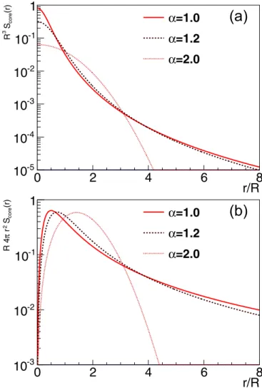
In principle, a more complete picture of the source geometry can be obtained by a three-dimensional Lévy analysis, utilizing Eqs. (49)–(52) of Ref. [40]. Given that the details of these studies go beyond the scope of the current paper, let us make only some general remarks here. If the source is a symmetric three-dimensional Gaussian, then in a one-dimensional anal- ysis (in ourQvariable, measured in the LCMS), one would obtainα=2 for the Lévy shape parameter. If the source is an asymmetric 3D Gaussian, then non-Gaussian 1D correlation functions would be obtained, but also strong deviations from the Lévy shape could be observed. We investigated this using the method of Lévy expansion of the correlation functions [55]
for eachmT bin, and found no first-order deviations from the Lévy shape. However, anmT averaged correlation function shows deviations from the pure Lévy shape, which may be attributed to the mT dependence of α. These observations suggest that the observed Lévy shapes do not originate from an asymmetric three-dimensional Gaussian source.
IV. STRENGTH AND SHAPE OF TWO-PION CORRELATION FUNCTIONS
We recapitulate some of the important general properties of the two-pion Bose-Einstein correlation functions. First, we discuss the strength of the correlation functions, and the main features of its interpretation, following the lines of Refs. [37,38]. Then we describe the shape assumption used in this paper, and the physical interpretation of the relevant parameters.
A. Correlation strength and its implications
If the final-state strong and Coulomb interactions can be neglected, then Eq. (14) implies that the correlation function takes the value 2 at vanishing relative momentum,C2(0)(Q= 0,K)=2. However, experimentally the two-track resolution (corresponding to a minimum value ofQmin of at least 6–8 MeV, depending on track momentum) prevents the measure- ment of correlation functions at Q=0. So the correlation function is measured at nonzero relative momenta and then extrapolated toQ=0. This extrapolated value in general can be different from the exact value atQ=0, and this can be quantified by defining
λ≡ lim
Q→0C2(Q,K)−1, (29) whereλmay depend on average momentumK.
In our analysis, we measure theC2correlation functions as a ratio of actual and background distributionsAandB, and we have carefully checked in our dataset that limQ→0A(Q,KT)
=0 and limQ→0B(Q,KT)=0 in every transverse momentum
range, indicating that the split tracks have been removed from our data sample. The two-track resolution, embodied into the values of two-track cuts as seen in Sec.III C, corresponds to a maximum spatial resolution ofRmax≈h/Q¯ min ≈25–30 fm.
In our analysis, source details on spatial scales larger or equal toRmaxcannot be experimentally resolved.
This (perhaps with different Rmax values) is a general feature of any similar experiment, and it leads to the core-halo picture of Bose-Einstein correlations in high-energy heavy-ion reactions [37,38]. The core-halo picture treats the particle emitting source as a composite one, corresponding to particle emission from a hydrodynamically behaving fireball-type core, surrounded by a halo of long-lived resonances. Such a picture is particularly relevant for pion production. Several long-lived resonances with decay widths of Qmin (like the η,η, KS0 mesons, and, depending on the experimental two-track resolution, maybe theωmeson) decay to pions that contribute to the halo region. The general structure of the core-halo model may hold not only for pion production but for the production of other mesons as well.
In short, limQ→0C2(Q,K)=1+λ(K) is in general dif- ferent from the exact value ofC2(Q=0,K) which (indepen- dently ofK) is 2 for a thermal, fully chaotic particle source.
In most data sets,λ <1 holds; see again the overview papers in Refs. [20,24–32].
In the core-halo picture, for thermal particle emission, the interceptλ, the extrapolation of the measuredresolvablepart of the correlation function to zero relative momentum, is the square of the fraction of pions coming from the core, defined as
fc≡ Ncore
Ncore+Nhalo, (30) because both pions have to come from the core if they are to contribute to the resolvable correlation function. This requires a physical assumption that the phase-space density of the pion- emitting source is made up of two components, i.e.,
S=Score+Shalo, (31) each component having a Fourier transform defined as
Score(q,K)≡
Score(x,K)eiqxd4x, (32) Shalo(q,K)≡
Shalo(x,K)eiqxd4x, (33) where we again used the four-vector variables q=p1−p2
and K=(p1+p2)/2. Then each component has a space- time integral corresponding to the contribution of the given component to the momentum distribution. We then may define
Ncore(K)≡
Score(x,K)d4x =Score(0,K), (34) Nhalo(K)≡
Shalo(x,K)d4x=Shalo(0,K). (35) Here the first equations in Eqs. (34) and (35) represent our physical assumption about the phase-space density of the core and the halo, while the second equations in Eqs. (34) and (35) indicate a mathematical identity about the Fourier transform.