József Smidla
Veszprém
2021
Numerically Stable Simplex Method Implementation
József Smidla Supervisors:
István Maros, DSc Tamás Terlaky, DSc
Doctoral School of Information Science and Technology University of Pannonia
Veszprém 2021
DOI:10.18136/PE.2021.801
NUMERICALLY STABLE SIMPLEX METHOD IMPLEMENTATION Thesis for obtaining a PhD degree in the Doctoral School of Information Science
and Technology of the University of Pannonia in the branch of Information Sciences
Written by: József Smidla Supervisors:
István Maros, DSc Tamás Terlaky, DSc
Proposes acceptance (yes/no)
Supervisor(s) As reviewer, I propose acceptance of the thesis:
Name of Reviewer: (yes/no)
Reviewer
Name of Reviewer: (yes/no)
Reviewer
The PhD-candidate has achieved % at the public discussion:
Veszprém,
Chairman of the Committee The grade of the PhD Diploma
Veszprém,
Chairman of the UDHC
The simplex method is one of the most important algorithms used to solve linear opti- mization problems (LO). Its development since the 1950s has been closely connected with the development of computer hardware and algorithms. While the first versions were only capable of solving small-scale problems, today’s software occasionally can handle problems even with millions of decision variables and constraints. However, solution of large scale optimization models may be problematic due to several reasons. Some of them can be attributed to the unavoidable use of floating-point arithmetic required by the solution algorithms. Though considerable progress has been made to alleviate these problems it is not uncommon that we encounter models that resist to the solution attempt. Great progress has also been achieved in dealing with models involving various numerical difficulties, such as scaling, perturbation, anti-degeneration strategies. It is important that these methods do not significantly slow down the completion of the entire task. But even the current software is unable to solve all the linear optimization problems correctly, as there are numerical errors that we cannot handle with traditional number representation. Existing software can also give poor results, such as cannot solve a prob- lem due to numerical difficulties or not converging to the optimum. This gave us the motivation to incorporate automatic features into our software (Pannon Optimizer) that can detect that the default floating-point number representation cannot solve the given model, so it is worth switching to more accurate arithmetic. This is a great help to the user as there is less doubt as to the correctness of the program output. In connection with this, we developed stable adder and dot-product implementations that do not contain conditional branching, so their computational overhead will be smaller. Moreover, we describe the acceleration method of one of the time consuming elementary steps of the simplex method. When discussing numerical algorithms, we provide information also on their speed efficiency.
A szimplex módszer az egyik legfontosabb algoritmus, amelyet a lineáris optimalizálási problémák (LO) megoldására használnak. Fejlesztése az 1950-es évek óta szorosan össze- függ a számítógépes hardverek és algoritmusok fejlesztésével. Míg az els˝o verziók csak kisméret˝u problémák megoldására voltak képesek, a mai szoftverek alkalmanként képe- sek kezelni olyan problémákat is, amelyek döntési változók millióiból és korlátozásaiból állnak. A nagyméret˝u optimalizálási modellek megoldása azonban több okból is prob- lematikus lehet. Ezek egy része a lebeg˝opontos aritmetika elkerülhetetlen használatának tulajdonítható, amelyet a megoldó algoritmusok megkövetelnek. Bár jelent˝os el˝orelépés történt e problémák enyhítése érdekében, nem ritka, hogy olyan modellekkel találkozunk, amelyek ellenállnak a megoldási kísérletnek. Nagy el˝orelépés történt a különféle nu- merikus nehézségekkel járó modellek kezelése terén is, például skálázás, perturbálás, degeneráció-ellenes stratégiák terén. Fontos, hogy ezek a módszerek ne lassítsák jelen- t˝osen az egész feladat megoldási folyamatát. De még a jelenlegi szoftverek sem képesek minden lineáris optimalizálási problémát helyesen megoldani, mivel vannak olyan nu- merikus hibák, amelyeket a hagyományos számábrázolással nem tudunk kezelni. A meglév˝o szoftverek gyenge eredményeket is adhatnak, például numerikus nehézségek miatt nem tudnak megoldani egy problémát, vagy nem konvergálnak az optimumhoz.
Ez adta a motivációt arra, hogy szoftverünkbe (Pannon Optimizer) beépítsünk olyan au- tomatikus eljárásokat, amelyek észlelhetik, hogy az alapértelmezett lebeg˝opontos ábrá- zolás nem tudja megoldani az adott modellt, ezért érdemes átállni a pontosabb számábrá- zolásra. Ez nagy segítség a felhasználó számára, mivel kevesebb kétség merül fel a pro- gram kimenetének helyességével kapcsolatban. Ennek kapcsán olyan stabil összeadó és skalár szorzat implementációkat fejlesztettünk ki, amelyek nem tartalmaznak feltételes elágazást, így számítási költségük kisebb lesz. Ezenkívül leírjuk a szimplex módszer egyik id˝oigényes elemi lépésének gyorsítási módszerét. A numerikus algoritmusok tár- gyalásakor ismertetjük a mérési eredményeinket is.
Simplexová metóda je jedným z najdôležitejších algoritmov používaných na riešenie problémov s lineárnou optimalizáciou (LO). Jeho vývoj od 50. rokov 20. storoˇcia bol úzko spätý s vývojom poˇcítaˇcového hardvéru a algoritmov. Zatial’ ˇco prvé verzie boli schopné riešit’ iba problémy malého rozsahu, dnešný softvér obˇcas dokáže zvládnut’
problémy aj s miliónmi rozhodovacích premenných a obmedzení. Riešenie vel’kých op- timalizaˇcných modelov však môže byt’ problematické z niekol’kých dôvodov. Niektoré z nich možno pripísat’ nevyhnutnému použitiu aritmetiky s pohyblivou rádovou ˇciarkou, ktorú vyžadujú algoritmy riešenia. Napriek tomu, že na zmiernenie týchto problémov bol urobený znaˇcný pokrok, nie je neobvyklé, že sa stretávame s modelmi, ktoré odolá- vajú pokusu o riešenie. Vel’ký pokrok sa dosiahol aj pri riešení modelov zah´rˇnajúcich rôzne numerické t’ažkosti, ako sú škálovanie, poruchy, stratégie proti degenerácii. Je dôležité, aby tieto metódy výrazne nespomal’ovali dokonˇcenie celej úlohy. Dokonca ani súˇcasný softvér nie je schopný správne vyriešit’ všetky problémy s lineárnou opti- malizáciou, pretože existujú numerické chyby, ktoré si s tradiˇcným zobrazovaním ˇcísel nevieme rady. Existujúci softvér môže tiež poskytovat’ zlé výsledky, napríklad nemôže vyriešit’ problém z dôvodu numerických problémov alebo nesúladu s optimom. To nás motivovalo zaˇclenit’ do nášho softvéru (Pannon Optimizer) automatické funkcie, ktoré dokážu zistit’, že predvolená reprezentácia ˇcísla s pohyblivou rádovou ˇciarkou nemôže vyriešit’ daný model, preto stojí za to prejst’ na presnejšiu aritmetiku. Je to vel’ká pomoc pre užívatel’a, pretože už nie sú žiadne pochybnosti o správnosti výstupu programu. V súvislosti s tým sme vyvinuli stabilné implementácie sˇcitaˇcky a skalárneho súˇcinu, ktoré neobsahujú podmienené vetvenie, takže ich výpoˇctová réžia bude menšia. Okrem toho popisujeme akceleraˇcnú metódu jedného z ˇcasovo nároˇcných elementárnych krokov sim- plexovej metódy. Pri diskusii o numerických algoritmoch poskytujeme informácie aj o ich rýchlosti.
Abstract iv
Abstract in Hungarian v
Abstract in Slovak vi
Acknowledgements xiii
Preface 1
Introduction 2
1 The simplex method 4
1.1 Short history . . . 4
1.2 Linear optimization problems . . . 4
1.3 The simplex method . . . 6
1.4 Product form of the inverse . . . 17
1.5 Computation of the reduced costs . . . 19
1.5.1 Reduced costs in phase-1 . . . 19
1.5.2 Reduced costs in phase-2 . . . 20
1.6 The dual simplex method . . . 22
1.7 Pannon Optimizer . . . 22
2 Floating-point numbers 24 2.1 A brief preview . . . 24
2.2 The floating-point format . . . 25
2.2.1 Rounding . . . 27
2.3 The IEEE 754 Standard . . . 33
3 Improvement techniques of pricing 37 3.1 Updating the phase-1 simplex multiplier . . . 37
3.2 Column-wise BTRAN algorithm . . . 40
3.3 Row-wise BTRAN algorithm . . . 44
3.4 Test results . . . 51
3.5 Major results and summary of accomplishments . . . 51
4.2 The Rounded Hilbert matrix . . . 60
4.2.1 Rounded Hilbert matrix example problem . . . 61
4.2.2 Analyzing the solutions . . . 65
4.2.3 Primary test . . . 69
4.3 Test results . . . 71
4.4 Major results and summary of accomplishments . . . 77
5 Low-level optimizations 78 5.1 Intel’s SIMD architecture . . . 78
5.2 Vector addition . . . 80
5.2.1 SIMD vector addition . . . 84
5.3 Vector dot-product . . . 86
5.4 Implementation details . . . 90
5.5 Computational experiments . . . 95
5.5.1 Vector addition . . . 96
5.5.2 Dot-product . . . 98
5.6 Conclusions . . . 98
5.7 Major results and summary of accomplishments . . . 99
Summary 100
A Column-wise and row-wise BTRAN test results 101
B Numerical error detector test results 105
C Low-level vector operation test results 117
D Orchard-Hays and simplified adder tests 132
E Some low-level vector implementations 136
F Abstract in Japanese 151
References 152
Index 161
List of Figures
1 Connections between the chapters . . . 3
1.1 Flow chart of the simplex method . . . 9
1.2 A simple linear optimization problem, and its MPS representation . . . 10
1.3 The simplified model after the presolver . . . 11
1.4 The scaled model . . . 11
1.5 The model with logical variables. In this example, y1and y2are the initial basic variables. . . 11
1.6 Computing phase-1 reduced cost vector using simplex multiplier rowwise matrix representation . . . 21
1.7 Pannon Optimizer architecture . . . 23
2.1 Convert 0.110to binary. . . 28
2.2 Different rounding modes. . . 29
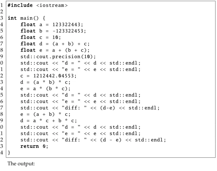
2.3 A short demo code in C++ to demonstrate the lack of associativity and distributivity. Compiled with gcc version 9.1.0. . . 30
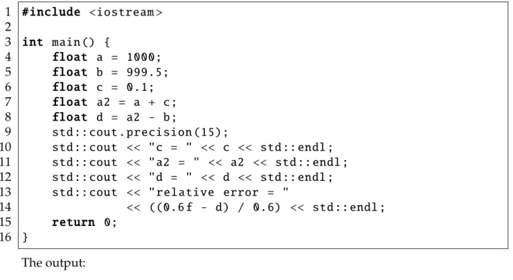
2.4 A short demo code in C++to demonstrate the cancellation error. Compiled with gcc version 9.1.0. . . 32
2.5 A short demo code in C++to demonstrate the double rounding. Compiled with gcc version 9.1.0. . . 36
3.1 Ab example for column-wise matrix representation . . . 39
3.2 Execution times of different sorting algorithms . . . 40
3.3 Example for a column-wise BTRAN implementation . . . 43
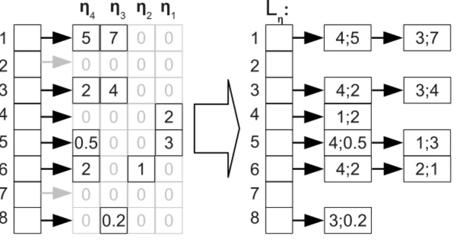
3.4 Theηvectors of example (3.3) using row-wise representation . . . 44
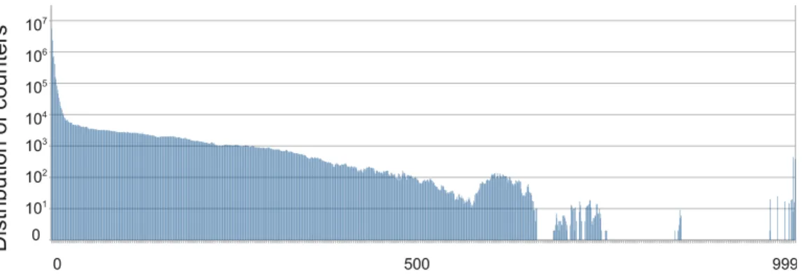
3.5 Distribution of nonzero products in STOCFOR2. The number of rows is 2156 45 3.6 Distribution of nonzero products in TRUSS. The number of rows is 999 . . 45
3.7 An example for the relationship ofLηandLaarrays . . . 46
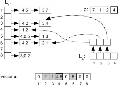
3.8 Extracting elements from the linked listLa[idx] . . . 47
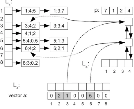
3.9 A new element was added to vectorasoLaalso gets a new element . . . . 48
3.10 The second element ofachanges, butLaremains the same . . . 48
3.11 Each data structure of the row-wise BTRAN algorithm . . . 50
3.12 Implementation of theLηlists . . . 51
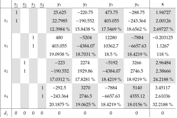
4.1 The starting tableau of the Rounded Hilbert matrix problem. The most infeasible variable isy1, andx1is the incoming variable. . . 65
4.2 The second tableau of the Rounded Hilbert matrix problem. The variable x1has a feasible variable, so the next outgoing variable is y3, andx2moves into the basis. The value ofy3 has a small relative error. . . 66 4.3 The third tableau of the Rounded Hilbert matrix problem. The outgoing
variable is y2, and x3 moves into the basis. The computation errors are more significant, for example, y4has a 1.25% of error. . . 67 4.4 The fourth tableau of the Rounded Hilbert matrix problem. The last out-
going variable is y4, andx4 moves into the basis. The computation errors are unacceptable, for example, the error of y4is 65.5%! . . . 68 4.5 The last tableau of the Rounded Hilbert matrix problem. The accumulated
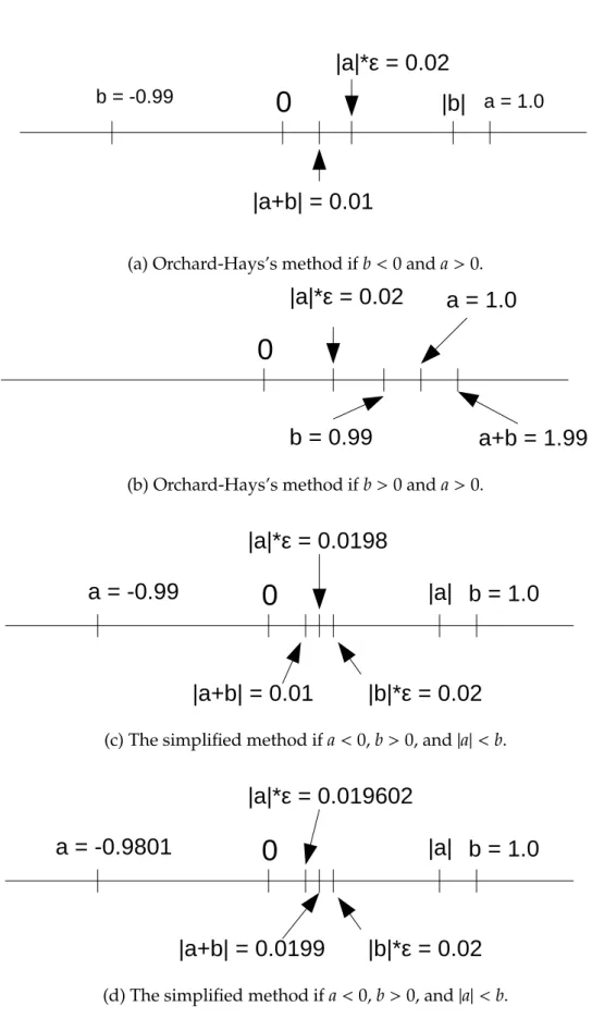
relative errors make our solution unusable. . . 69 5.1 Addition using XMM registers . . . 78 5.3 The red area is the small range where the two methods give a different
result. The Orchard-Hays’s method goes to zero in the blue and red ranges, while the simplified method moves to zero only in the blue area. . . 82 5.2 Comparison of Orchard-Hays’s and the simplified addition algorithms.
For the sake of simplicity,λ=1 andǫ=0.02. . . 83 5.4 The compare instruction of the SSE2 instruction set . . . 84 5.5 Flow chart of the stable add implementation, using absolute tolerance.
Arrow numbers show the order of the operations. . . 87 5.6 Flow chart of the stable add implementation, using relative tolerance. Ar-
row numbers show the order of the operations. . . 88 5.7 Handling positive and negative sums with pointer arithmetic without
branching, where S is the sign bit, M is the significand and E is the ex- ponent . . . 90 5.8 Flow chart of the stable dot product implementation. Arrow numbers
show the order of the operations. . . 91 5.9 The source code of the naive SSE2 version vector-vector add template
function. . . 93 5.10 The source code of the naive SSE2 version vector-vector add functions,
with caching and non-caching versions. . . 94 C.1 Performances of the unstable add vector implementations for three vectors 117 C.2 Performances of the stable add vector implementations, using relative tol-
erance, for three vectors . . . 118 C.3 Performances of the stable add vector implementations, using absolute
tolerance, for three vectors . . . 118 C.4 Performances of the unstable add vector implementations for two vectors 119 C.5 Performances of the stable add vector implementations, using relative tol-
erances for two vectors . . . 119 C.6 Performances of the stable add vector implementations, using absolute
tolerance, for two vectors . . . 120
C.8 Performance comparison of our stable add implementations and the method of Orchard-Hays, with AVX, using relative tolerance, for three vectors . . 121 C.9 Performance comparison of our stable add implementations and the method
of Orchard-Hays, with SSE2, using relative tolerance, for two vectors . . . 121 C.10 Performance comparison of our stable add implementations and the method
of Orchard-Hays, with AVX, using relative tolerance, for two vectors . . . 122 C.11 Performance ratios relative to the naive versions, with 3 vectors . . . 122 C.12 Performance ratios relative to the naive versions, with 2 vectors . . . 123 C.13 Performances of the dot product implementations . . . 123 C.14 Performances of the unstable add vector implementations for three vectors,
on Xeon Platinum . . . 124 C.15 Performances of the stable add vector implementations, using relative tol-
erance, for three vectors, on Xeon Platinum . . . 124 C.16 Performances of the stable add vector implementations, using absolute
tolerance, for three vectors, on Xeon Platinum . . . 125 C.17 Performances of the unstable add vector implementations for two vectors,
on Xeon Platinum . . . 125 C.18 Performances of the stable add vector implementations, using relative tol-
erances for two vectors, on Xeon Platinum . . . 126 C.19 Performances of the stable add vector implementations, using absolute
tolerance, for two vectors, on Xeon Platinum . . . 126 C.20 Performance comparison of our stable add implementations and the method
of Orchard-Hays, with SSE2, using relative tolerance, for three vectors, on Xeon Platinum . . . 127 C.21 Performance comparison of our stable add implementations and the method
of Orchard-Hays, with AVX, using relative tolerance, for three vectors, on Xeon Platinum . . . 127 C.22 Performance comparison of our stable add implementations and the method
of Orchard-Hays, with SSE2, using relative tolerance, for two vectors, on Xeon Platinum . . . 128 C.23 Performance comparison of our stable add implementations and the method
of Orchard-Hays, with AVX, using relative tolerance, for two vectors, on Xeon Platinum . . . 129 C.24 Performance ratios relative to the naive versions, with 3 vectors, on Xeon
Platinum . . . 130 C.25 Performance ratios relative to the naive versions, with 2 vectors, on Xeon
Platinum . . . 130 C.26 Performances of the dot product implementations . . . 131
1.1 Types of variables . . . 7
1.2 Rules of finding an improving variable in phase-1 . . . 12
1.3 Rules of finding an improving variable in phase-2, with a minimization objective function. Obviously, the maximization problems have opposite rules. . . 13
2.1 Different representations of the numberx=123.625. . . 26
2.2 The main IEEE 754-2008 radix-2 floating-point formats. . . 32
4.1 Condition numbers . . . 61
4.2 Differentbinput vectors and solution vectors of a Rounded Hilbert matrix problem, after 4 iterations . . . 64
4.3 Reinversion times using different number representations. . . 70
4.4 Comparison of different size of Rounded Hilbert matrix problems with 3 softwares. . . 73
4.5 Comparison of different size of Rounded Pascal matrix problems with 3 softwares. The right outputs are underlined. . . 75
4.6 Summarized execution times and iteration numbers in different test con- figurations. . . 76
List of Algorithms
2.1 Convert decimal fractional number to binary . . . 283.1 Algorithm for computingφT(B−B)e¯ p . . . 41
3.2 BTRAN algorithm using column-wiseηrepresentation . . . 42
3.3 Pseudo code of the row-wise BTRAN algorithm . . . 49
4.1 Computing the vectorb, naive version . . . . 63
4.2 Computing the vectorb, adding in increasing order . . . . 63
4.3 Computing the vectorb, Kahan’s algorithm . . . . 64
5.1 Naive vector addition . . . 81
5.2 Vector addition using absolute tolerance . . . 81
5.3 Vector addition using relative tolerance, Orchard-Hays’s method . . . 81
5.4 Vector addition using simplified relative tolerance . . . 82
5.5 Naive dot-product . . . 86
5.6 Stable dot-product, whereStableAddis an implementation of the addition, which can use tolerances . . . 89
In this way, I would like to thank my supervisor, Professor Dr. István Maros, for his many years of joint work, his many useful guides, his experiences and for providing a calm and supportive atmosphere during my research work. Special thanks to the Department of Computer Science and Systems Technology, Faculty of Information Technology, Univer- sity of Pannonia for giving me the opportunity as a first-time student to participate in teaching and research in addition to studying. I am grateful to the members of the Op- erations Research Laboratory for their extraordinarily inspiring joint work, namely Péter Tar, Bálint Stágel and Péter Böröcz. One of my important results would not have been possible if I had not participated in the work of the Wireless Sensor Networks Laboratory led by Dr. Simon Gyula for a short time.
Writing my dissertation was hampered by numerous obstacles, so I would like to thank all my friends, colleagues and family members who had the patience and understanding for the missed meetings and joint programs. I would like to thank Dr. Máté Hegyháti, Dr. Máté Bárány and Dr. Gergely Vakulya for their moral encouragement and Dr. Anikó Bartos for all the useful information. Thanks to Anita Udvardi and Nader Abdulsamee for proofreading the English text, and Balázs Bosternák for translating the Slovak abstract.
I would not have been able to perform some of the tests in the dissertation without the support of Zoltán Ágoston and KingSol Zrt.
Linear optimization models
m Number of constraints
n Number of decision variables, dimension ofx x Vector of decision variables
xj Decision variable j
ℓ Vector of lower bounds of variables u Vector of the upper bounds of variables c Coefficient vector of the objective function z Value of objective function
L Vector of the lower bounds of constraints U Vector of the upper bounds of constraints aij The jth coefficient in theith constraint A Matrix of constraints
χ Set of feasible solutions Simplex method
y Vector of logical variables
I Identity matrix
b Right hand side of constraints in transformed computational form
B Basis part ofA
R Nonbasis part ofA
N Set of indices of variables B Set of indices of basic variables
R Set of indices of nonbasic variables
U Set of indices of nonbasic variables, at upper bound xB Vector of basic variables
xR Vector of nonbasic variables
cB Coefficient vector of basic variables cR Coefficient vector of nonbasic variables β Vector of values of basic variables B−1 Inverse of the basis
αj The jth transformed column of matrixA θ Steplength of a nonbasic variable
w Measure of infeasibility
M Set of indices of basic variables below their lower bound P Set of indices of basic variables above their upper bound dj Reduced cost of the jth variable
z Value of updated objective value
η Non-unit column of an elementary transformation matrix E Elementary transformation matrix
s number of the ETMs
dˆj Normalized reduced cost of the jth variable σj Direction of changingx, whenxjchanges by 1
h Auxiliary vector
φ Simplex multiplier in phase-1 π Simplex multiplier in phase-2 ρp Thepth row of inverse of the basis ρ¯p The updatedpth row of basis inverse Numerical stability
κ(M) Condition number of the matrixM
Other symbols
R Set of real numbers
kvk2 Euclidean norm of vectorv ej Unit vector
Text formatting
In this dissertation we follow the following text formatting conventions:
• The first occurrences of important keywords are initalics.
• C++source codes, source code snippets, program variables, and program outputs are formatted bytypewriterfont:
1 # include < iostream >
2
3 int sum (int a , int b) { 4 if (! a) {
5 return b;
6 }
7 return sum (( a & b) << 1, a ^ b );
8 } 9
10 int main () {
11 std :: cout << " The sum : " << sum (10 , 20) << std :: endl ; 12 return 0;
13 }
The output:
The sum: 30
• The mathematical expressions, formulas, variables, symbols are in mathematical form: eiπ+1=0
Over the past 70 years, linear optimization has remained one of the essential tools in operations research. Its use is critical in proper economic decision-making processes, so its research results in significant benefits. Its development is closely related to the development of computer technology, so with more advanced technology we can solve more problems more efficiently. This supports faster decision-making process.
I have come across a few times a mathematical model (Rump’s matrices, discrete moment problems, or some industrial models) for which existing solver software (like GLPK and COIN-OR) gave the result that it is infeasible or unbounded while examining the models revealed that this is not the case: the software gave a wrong result. The problem was caused by the numerical instability of the coefficient matrix. This gave me the motivation to incorporate automatic features into our software (Pannon Optimizer) that can detect that the default floating-point number representation cannot solve the given model, so it is worth switching to more accurate arithmetic. This is a great help to the user as there is less doubt as to the correctness of the program output. Related to this, I also turned to speed up stable operations: during a professional conversation, a developer of a well-known software explained to me that they don’t use stable addition algorithms because they interfere with the CPU pipeline mechanism. The idea of a C- language implementation of a branchless dot-product came to me at this time, and then I developed further implementations as well.
The simplex method is one of the most important algorithms used to solve linear optimiza- tion problems. While the first computer implementations in the 1950s were only capable of solving small-scale problems, today’s software occasionally can handle problems even with millions of decision variables and constraints. But even though many algorithms have been added to the original simplex method with which we can handle many numeri- cal problems, even today’s solver software is not able to solve all the problems. Therefore, our primary goal was to create a new algorithm that allows the software to detect that it is working on a numerically too unstable problem and can inform the user accordingly.
To present our work, we discuss the simplex method to the necessary depth in Chapter 1, and we shortly introduce our simplex implementation named Pannon Optimizer. This method is also forced to use fractional numbers, and processors support floating-point number representation, and it is best suited for scientific calculations. Since this number representation is the cause of the numerical problems examined in the dissertation, we will describe them in Chapter 2. In the later chapters, we will build heavily on these properties and number representation: To understand the numerical problems described in the later chapters, it is necessary to know the properties and problems of floating-point numbers and the IEEE 754 Standard. In Chapter 3, we present the acceleration of the most time-consuming and numerically critical step of the simplex method. In Chapter 4, we describe the condition numbers of the matrices and then prove that it is not enough for our solving software to draw conclusions from the numerical properties of the input matrix. We then propose a method by which the solving software adapts to the numerical properties of the problem that has to be solved and, if necessary, checks the numerical quality of the current inverse of the basis representation. If the checker finds that the current inverse of the basis is numerically unusable, this indicates that the software can then switch to a slower but a more reliable number representation. As a result, unlike the solving software that is used currently, the user does not get false results. Finally, in Chapter 5, we describe a few low-level, numerically stable vector-vector adder and dot-product implementations based on Intel’s SIMD instruction set which are much faster than the simple C++ implementations. We also describe and examine a simplified but faster version of Orchard-Hays’s classic stable adder. We use measurements to prove that our own simplified algorithm is faster, and we still get correct result.
Figure 1: Connections between the chapters
The simplex method
In this chapter, we introduce the linear programming problems and the simplex method.
1.1 Short history
The history of linear programming began in 1939 [21], when the Soviet Kantorovich published his method that solved a general linear programming problem [43] He used this method to optimize military operations during the war. However, his work was neglected in the Soviet Union, his results only became known in the West in 1959 [16]. Meanwhile,Dantzigindependently developed the formulation of the general linear programming problems in the US Air Force [18] in 1947 and he later published the simplex method [14]. John von Neumann had conjectured the theorem of duality at a meeting with Dantzig [18].
It seemed that the simplex method is a polynomial algorithm, but in 1972 Klee and Minty proved that in specific problems the simplex method is exponential [47]. Khachiyan published his ellipsoid method in 1979, which was polynomial algorithm [45]. However, this algorithm was slower in most of the linear programming problems. In 1984 Kar- markar introduced the interior-point method which was a highly efficient, polynomial algorithm [44]. Later, in 1985 and 1987 Terlaky published the Criss-Cross algorihm [96], [97].
1.2 Linear optimization problems
In linear optimization (or linear programming), modelers describe problems with linear expressions, linear inequalities. The solution to the problem is represented by numerical values, so we need an n-dimensional vector that contains the decision variables, denoted byx. Each variable has an individuallower boundandupper boundfrom the set of{−∞,R} and{+∞,R}respectively. If the variable satisfies its bounding criterion, then it is afeasible variable. The ndimensional ℓvector contains the lower bounds anduconsists of upper bounds. We can say that the variable has no lower /upper bound if the corresponding bound is−∞/ +∞. Obviously,ℓj ≤uj.
ℓj ≤xj ≤uj,j=1. . .n (1.1) The value we wish to minimize or maximize is the objective function which is the linear combination of the decision variables. Thendimensionalcost vectorccontains the coefficients of the variables in the objective function, so formally the objective function is the following:
minz=
Xn j=1
cjxj (1.2)
or we can define a maximization problem:
maxz=
Xn j=1
cjxj (1.3)
But it is known, that there is a simple connection between minimization and maximization problems:
minz= −max −z (1.4)
Therefore, throughout the rest of this dissertation we can talk about minimization prob- lems without loss of generality.
If we would like to solve real-life problems, we have to take into consideration certain restrictions: The problems have constraints too, which are expressed by linear inequalities constructed fromx: For the linear combination ofxwe can give lower and upper bounds.
Letmdenote the number of constrains. We can write the constraints formally as follows:
L1 ≤x1a11+. . .+xna1n≤U1
...
Li ≤x1ai1+. . .+xnain≤Ui
...
Lm ≤x1am1 +. . .+xnamn ≤Um
where the mdimensional vectors L and U contain the lower and upper bounds of the constraints. Theaij is the coefficient of jth variable inith constraint where 1 ≤i ≤mand 1 ≤ j ≤ n. The matrix Am×n contains these coefficients. The linear optimization model is composed of the variables, the objective function and the constraints:
minz= cTx (1.5)
s.t. L≤Ax≤U (1.6)
ℓ≤x≤u (1.7)
If xsatisfies the inequality system (1.6), it is asolution. Ifxis a solution and satisfies (1.7), then it is afeasible solution. Theχdenotes the set of feasible solutions:
χ={x: L≤Ax≤U, ℓ≤x≤u} (1.8) The problem has no feasible solution, if and only ifχ=∅. The solutionx∈χisoptimal, if: ∀x′ ∈χ: cTx≤cTx′.
1.3 The simplex method
In this section, we introduce the simplex method. First, we describe the computational form of the linear optimization model as well as the principle of solver algorithm, and finally, we briefly explain the modules . From a mathematical point of view, there are two versions of the simplex method: Theprimal[14] anddual[55]. We notice thatMaros introduced a general dual phase-2 algorithm in 1998 [60], and later in 2003 the general dual phase-1 [59], which iterate faster to the optimum. In this dissertation we only discuss the primal method in details.
Previously, we saw the general form of linear optimization problems in (1.5) - (1.7), but we need to transform this into a simpler but equivalent form. There are two reasons for this transformation: First, it makes the introduction of the algorithms easier to discuss, and second, the source code of the software becomes simpler.
Severalcomputational formsexist, and they have a common property: The constraints are transformed into equality by introducinglogical variables. These special variables are contained by themdimensional vectory. In some forms, we need to translate the lower and upper bounds of variables, too. The transformed computational form we will use in this dissertation is the following:
minz= cTx (1.9)
s.t. Ax+Iy=b (1.10)
type(xj),type(yi)∈ {0,1,2,3},1≤ j≤n,1≤i≤m (1.11) In the applied computational form, we allow the following types of variables:
Hereafter, we will use as acoefficient matrixas follows:
A:=[A|I]
Feasibility range Type Reference yj,xj =0 0 Fixed variable 0≤ yj,xj ≤uj 1 Bounded variable 0≤ yj,xj ≤+∞ 2 Nonnegative variable
−∞ ≤ yj,xj ≤+∞ 3 Free variable Table 1.1: Types of variables and moreover the
x:=
x y
vector will contain the variables, and the cost coefficients belonging to the logical variables are zero:
c:=
c 0
For the simplex method, we partition the Amatrix into two sections, theB,basisand theRsubmatrix, which contains columns fromAthat are not inB:
A=[B|R]
For notational simplicity, we need some index sets. Let N denote the index set of the variables. Each variable is associated with a column of matrix A. We say that when a column is in the B basis, then the corresponding variable is also in the basis . These are thebasic variables, others are the nonbasic variables. The setBcontains the indices of basic variables, whileRcontains indices of nonbasic variables. Moreover, setUdenotes the indices of nonbasic variables, which are at their upper bound. From the previous observation, we can splitxinto basic variables and nonbasic variables, respectively:
x=
xB xR
Similarly, we also splitc:
c=
cB cR
We can show that in an optimal solution, the nonbasic variables are at their bounds, and the values of basic variables are determined by the nonbasic variables as follows:
β =xB =B−1(b−RxR) (1.12)
We need the following notation: Letαj denote the product of jth matrix column and basis inverse:
αj =B−1aj (1.13)
Two bases are called neighboring bases when they differ from each other in only one column. We can move from a basis to a neighboring one by a so-called basis change.
The principle of the simplex method is the following: Determine a starting basis and search the optimal solution through a finite number of basis changes. The optimality of a solution can be verified easily; the simplex method guarantees that it is a global optimum. Usually, when the algorithm starts from an infeasible solution, the so-called primal phase-1 controls the basis changes: Its task is to find a feasible solution. Maros introduced a phase-1 algorithm in 1986 [58]. After a feasible solution is found, variables are kept in feasible ranges byprimal phase-2, while searching for an optimal solution. For the sake of simplicity, we focus on phase-2 in this dissertation.
In each iteration, the simplex algorithm affects the value of a chosen nonbasic variable, and in many cases, this variable moves into the basis. Let xq be the chosen nonbasic variable, andθdenotes thesteplengthof the change inxq. In this case, the basic variables change as shown by the following formula:
β=β−θαq (1.14)
Since θaffects feasibility, during the computation ofθwe have to take into consider- ation that the solution has to stay feasible.
Now we introduce the major steps of the simplex algorithm. Figure (1.1) shows these steps and their logical connections.
MPS reader
Most of the linear optimization problems can be found in standardized text files. There are numerous file formats, and the most common file format is the MPS. Every simplex implementation has to support the MPS (Mathematical Programming System) format.
The MPS was the first format designed for linear optimization systems at the age of punched cards, so this caused a very rigid storage method. Figure (1.2) shows a simple example LO problem and its MPS representation. Notice that the cost coefficients are multiplied by -1 according to (1.4) because the MPS format describes only maximization problems. Later on, technical development allowed using other, advanced, and more sophisticated formats, but there were too many models in MPS, so this legacy format remained the de-facto standard format of LP models. However, the usage of this format has declined, because of the wide acceptance of the algebraic modeling languages, like AMPL [42] and GAMS [24]. The task of the MPS reader is to read these files, detect their errors, and compute statistics. The result of this module is the raw model, which is stored in the memory. The following software modules will perform transformation operations and computations on this raw model.
Figure 1.1: Flow chart of the simplex method Presolver
From the mathematical point of view, thepresolveris not a necessary module of the simplex algorithm. The task of the presolver is simplification and improvement of the model.
Since some generator algorithms create many models, the model may be redundant. The presolver algorithm has to recognize the removable columns and rows in such a way that the resulting model is equivalent to the original one.
For example, a basic presolver can simplify the LO model introduced formerly in Figure (1.2); it recognizes that the 3rd row is unnecessary; that is, it defines an upper bound for the variable x2. The presolver removes the 3rd constraint and modifies the upper bound ofx2, as it can be seen in Figure (1.3). In the example, the coefficient matrix’s size decreased; therefore, the simplex algorithm can work faster.
After the solver algorithm found an optimal solution, the so-called postsolver (the pair of presolver) has to insert the removed variables back into the model to represent the solution for the user by the original model. The first publication about the presolver was the work ofBrearley, Mitra and Williamsin 1975 [5], it was followed byTomlinand Welch’s article in 1983 [101, 100], Andersen andAndersenin 1995 [3], andGondzioin 1997 [29]. The last two results apply to interior-point methods.
maxz: 600x1+800x2
40x1+20x2 ≤ 550 32x1+64x2 ≤ 150 48x2 ≤ 120 x1,x2≥0
NAME demo
ROWS L c1 L c2 L c3 N z COLUMNS
x1 c1 40 c2 32
x1 z 600
x2 c1 20 c2 64
x2 c3 48 z 800
RHS
RHS1 c1 550 c2 150
RHS1 c3 120
ENDATA
Figure 1.2: A simple linear optimization problem, and its MPS representation
Scaler
Like the presolver, the scaler is also an optional module, executed before the simplex algorithm. There are LO problems, where the variance of the entries ofAis too large, so this can increase the numerical instability of the algorithm. The scaler created to stabilize the numerically unstable problems; scales the rows and columns of the matrix to decrease the variance as much as possible. We scaled our example model in a way that is using powers of 2, to avoid additional numerical errors, using the method that was proposed by Benichou in [4]; the variance of matrix elements is reduced. Figure (1.4) shows the result.
Finding the starting basis
As we saw in Figure (1.1), before the iterative part of the algorithm, we need to select a reasonable starting basis. There are numerous ways to select a starting basis. The most straightforward way is to select the identity matrix; namely, we select only logical variables into the basis. This is called alogical basis. The logical basis is simple and easy to implement, but we can construct bases that are probably closer to an optimal solution, so researchers have designed many starting basis finder algorithms, with different ad-
maxz: 600x1+800x2
40x1+20x2 ≤ 550 32x1+64x2 ≤ 150 48x2 ≤ 120 x1,x2≥ 0
=⇒
maxz: 600x1+800x2
40x1+20x2 ≤ 550 32x1+64x2 ≤ 150 x1 ≥0,0≤x2 ≤2.5
Figure 1.3: The simplified model after the presolver
maxz: 600x1+800x2
40x1+20x2 ≤ 550 32x1+64x2 ≤ 150 x1 ≥0,0≤x2 ≤2.5
=⇒
maxz: 600x1+800x2
1.25x1+0.625x2 ≤ 17.1875 0.5x1+x2 ≤ 2.34375 x1 ≥0,0≤x2 ≤2.5
Figure 1.4: The scaled model
vantages; minimizing the infeasibility, degeneracy, and so on. The algorithm also creates the logical variables at least here, and converts ≤and ≥constraints into =equations, as Figure (1.5) shows. Finally, this module initializes the values of nonbasic variables into one of their bound.
max z: 600x1+800x2
y1 + 1.25x1 + 0.625x2 = 17.1875 y2 + 0.5x1 + x2 = 2.34375 x1 ≥0,0≤ x2≤2.5,y1,y2 ≥0
Figure 1.5: The model with logical variables. In this example, y1
and y2are the initial basic variables.
The simplex algorithm executes the following modules in every iteration, so their implementations have to be very efficient.
Feasibility test
The values of the nonbasic variables determine the values of basic variables, as (1.12) shows. The solver has to check whether these values violate their feasibility range or not; that is, whether the solution is feasible or not. When the solution is infeasible, this module prepares special data structures for phase-1 algorithms. In theory, we skip this step in phase-2, but practical experiences show that we have to perform afeasibility testin both phases: Numerical errors can occur and lead to infeasible solutions, pushing back the solver to phase-1.
Let M and P denote the index sets of infeasible basic positions, where i ∈ M, if the ith basic variable is below its lower bound, andi∈ Pif theith basic variable is above its
upper bound. We need a phase-1 objective function, which summarizes these feasibility range violations:
w=X
i∈M
βi−X
i∈P
(βi−vi)
When w < 0, then the actual solution is infeasible, because there is a basic variable, which is below its lower bound or above its upper bound. The task of pricing is to choose a nonbasic variable for increasing the value of w. We can calculate aphase-1 reduced cost for each nonbasic variable:
dj =X
i∈M
αij−X
i∈P
αij (1.15)
The meaning of this reduced cost is the following: Whenxqis increased by t, butM and P still remain unchanged, then the value of w changes by −tdq: ∆w = −tdq. When t is negative, pricing has to choosexq in such a way thatdq < 0, but whent is positive, we need a positive dq. We summarized the choosing rules for different cases in table (1.2): When the pricing cannot find an appropriate nonbasic variable andw<0, then the
Type Value dj Improving displacement Remark
0 xj =0 Irrelevant 0 Never enters to basis
1 xj =0 <0 +
1 xj =uj >0 − j∈ U
2 xj =0 <0 +
3 xj =0 ,0 +/−
Table 1.2: Rules of finding an improving variable in phase-1 algorithm halts, the problem has no solution.
Pricing
In the primal simplex, the pricing selects a nonbasic variable xk candidate to enter the basis; we say that it is an incoming variable. With moving the incoming variable, the objective function has to improve. We compute a phase-2 reduced cost for each j ∈ R nonbasic variable based on the following formula:
dj =cj−cTBB−1aj (1.16) The Formula (1.16) comes from these:
z=cTBxB+cTRxR (1.17)
xB=B−1(b−RxR) (1.18)
If we mix these formulas and rearrange them, we get the following:
z=cTBB−1b+(cTR−cTBB−1R)xR (1.19) Since according to (1.19)z=cTx, , ifxk(k∈ R) changes byθ, then
z(θ)=z+θdk (1.20)
As (1.20) shows, the reduced costs determine the direction of the objective function’s change. Therefore, we can introduce the so-called optimality conditions; if and only if there are no more improving variables (see Table (1.3), the current solution is optimal.
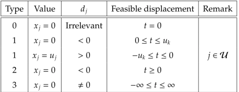
Type Value dj Feasible displacement Remark 0 xj =0 Irrelevant t=0
1 xj =0 <0 0≤t≤uk
1 xj =uj >0 −uk ≤t≤0 j∈ U
2 xj =0 <0 t≥0
3 xj =0 ,0 −∞ ≤t≤ ∞
Table 1.3: Rules of finding an improving variable in phase-2, with a minimization objective function. Obviously, the maximization problems have opposite rules.
In our example, the starting basis consists of the logical variables:
B=(y1,y2)⇒B=
1 0 0 1
,cB =
0 0
R=(x1,x2)⇒ R=
1.25 0.625
0.5 1
,cR =
600 800
The right-hand side vector is constant:
b=
17.1875 2.34375
The nonbasic variables are in their bound:
xR=
x1 =0 x2 =0
Based on Formula (1.12), we can compute the basic variables:
β =xB=B−1(b−RxR)=
y1= 17.1875 y2= 2.34375
Obviously, the initialzvalue is 0.
The variables satisfy their bound criterion, so this is a feasible solution; we are in phase-2, we can calculate the phase-2 reduced costs based on Formula (1.16):
dT =cTR−cTBB−1R=
dx1 =600 dx2 =800
As Table (1.3) shows (recall that we have a maximization problem now), both nonbasic variables are good candidates to enter the basis. There are numerous variants of pricing strategies, the simplest one is the Dantzig pricing [14]: We choose the variable to have the largest reduced cost. However, there are other advanced strategies as well. The most common methods are the normalized pricing strategies; Harris introduced the Devex in 1973 [30], and Goldfarb and Reid developed the Steepest-edge in 1977 [28].
In our case, we simply choose x2 to enter the basis, its reduced cost is 800, and let denoteq=2 the incoming variable’s index. As the corresponding
αq=B−1aq=
0.625
1
,
we have to choose a basic variable, which leaves the basis.
Ratio test
The pricing selects a variable to enter the basis. Theratio testhas to determine the outgoing basic variable in a way that the feasibility ranges are maintained in phase-2, or decrease feasibility violations in phase-1. But sometimes it happens that the basis change is not possible. In this case, we perform a bound flip operation; change the incoming variable from its lower bound to the upper one, or vice versa.
Recall Formula (1.14), and keep in mind that the simplex algorithm has to modify the basic variables in a way that they still have to stay inside their feasible range:
li ≤βi−Θαiq≤ui
where li and ui are the lower and upper bounds of the ith basic variable. We have several such inequalities, but only oneΘ that we are looking for; we have to solve these inequalities to obtain different possibleΘ values, and finally we choose their minimum.
If we select this value properly, this displacement moves one basic variable into its bound, and that variable leaves the basis.
In our example there are 2 basic variables, the y1 and y2, and they have only a lower bound, so there are 2 inequalities:
0≤β1−Θ1α1q →0≤17.1875−Θ10.625→Θ1 =27.5 0≤β2−Θ2α2q →0≤2.34375−Θ2→ Θ2=2.34375
The Θis theΘ2, and the outgoing variable is the y2. We say that, this variable is the pivot element, andp=2.
Basis change
This module performs a basis change: It removes the outgoing variable from the basis, and inserts the incoming variable. Finally, it updates a few data structures, for example, the values of basic variables. When it is necessary, this module performs thereinversion of the basis. For higher efficiency, we can integrate the feasibility test in this module.
As saw in the previous subsections, in the example problem, the incoming variable is the x2, and y2 leaves the basis. So this step modifies the list of basic and nonbasic variables, and updates other data structures:
B=(y1,x2)⇒B=
1 0.625
0 1
,cB =
0 800
R=(x1,y2)⇒R=
1.25 0 0.5 1
,cR=
600
0
We update the basic variables according to Formula (1.14), and the basic variable at the pivot position changed byΘ:
β=xB =
y1 =15.72266 x1=0→2.34375
The objective function’s value grows from zero: z=z+ Θdq=2.34375·800=1875. As one can see, the algorithm has to make logical decisions in several places, namely based on reduced costs,α, andβvectors. In Chapter 4, we will see that if we make a significant numerical error in any of its calculations, the algorithm will continue the calculation in the wrong direction. This can result in cycling or an erroneous result.
Finishing the example
Fortunately, the variables are in their feasible range, so we can compute the new reduced costs:
dT =
600 0
−
0 800
1 0.625
0 1
−1
1.25 0 0.5 1
=
200 −800
The only one improving variable is the x1, which reduced cost is 200, soq = 1. The associatedα1 =B−1a1 =
1 0.625
0 1
−1
1.25
0.5
=
0.9375
0.5
. In the ratio test 2 inequalities have to be solved:
0≤15.72266−Θ10.9375→ Θ1= 16.77083
0≤2.34375−Θ20.5→ Θ2= 4.6875
Notice that x2 has an upper bound, but the corresponding αi value is positive, so this variable moves towards its lower bound. The current Θ = 4.6875, and p = 2. The new basic variables after the basis change:
β=
11.32813 4.6875
The objective function grows again:
z=1875+4.6875∗200=2812.5 The new basis, and the other data structures changes as follows:
B=(y1,x1)⇒B=
1 1.25 0 0.5
,cB=
0 600
R=(x2,y2)⇒R=
0.625 0
1 1
,cR=
800
0
The new reduced costs:
dT =
800 0
−
0 600
1 1.25 0 0.5
−1
0.625 0
1 1
=
−400 −1200
Finally, as the reduced costs are -400 and -1200, there are no more improving variables,
an optimal solution has been found.
1.4 Product form of the inverse
During the solution algorithm the vector-matrix and matrix-vector products with theB−1 matrix are widely used:
α=B−1a (1.21)
πT =hTB−1 (1.22)
We can update B−1 in each iteration, and perform the multiplications, but keeping B−1 up to date is very time consuming. The so-called Product Form of Inverse (PFI) representation (PFI) of the basis developed by Dantzig and Orchard-Hays is a proper way to handle this problem [17, 61, 15]. We notice that, later onMarkowitzpublished the LU decomposition method [57], but we omit that in this dissertation. The principle of PFI is thatB−1can be represented by the product ofelementary transformation matrices(ETMs):
We store the ETMs in a list, and at basis change the algorithm appends a new ETM to the end of list. An ETM can be determined quickly. When the algorithm has to compute (1.21), we use theFTRANalgorithm, and for (1.22) we need theBTRANalgorithm.
Let Bbe the original basis matrix, andBα is the neighbor of B, the bases differ from each other in thepth column, because the algorithm changed thepth column ofBby an avector.
B=h
b1, . . . ,bp−1,bp,bp+1, . . . ,bm
i
⇓ Bα =h
b1, . . . ,bp−1,a,bp+1, . . . ,bm
i
For constructing the new ETM, we will need the v = B−1a vector, which can be computed by the ratio test. Computing theηvector fromvis as follows:
η=
"
−v1
vp
, . . . ,−vp−1
vp
, 1
vp − vp+1
vp
, . . . ,−vm
vp
#
TheEETM is the following:
E=
1 η1
. .. ...
ηp ... . ..
ηm 1
By usingEmatrix,B−α1 can be computed with the following formula:
B−1α =EB−1
After theith basis change the basis inverse is the following:
B−i1 =EiEi−1. . .E1, where
B−01 =I
For FTRAN and BTRAN it is sufficient to store the η vectors and the corresponding p indices from ETMs.
FTRAN
The FTRAN (Forward Transformation) operation implements the (1.21) formula. Suppose that, the actual basis is represented by product ofsETMs. We know that
α=B−1a=EsEs−1. . .E1a (1.23)
α0=a
αi =Eiαi−1,i=1, . . . ,s αs=α
Theα=Eacan be performed by the following:
α=Ea=
1 η1
. .. ...
ηp ... ...
ηm 1
a1
... ap
...
am
=
a1+η1ap
... ηpap
...
am+ηmap
Notice that, whenap =0, then the we can omit the related ETM from (1.23).
BTRAN
We use the BTRAN (Backward Transformation) for the (1.22) formula. The inverse of the basis is represented bysETMs. We know that
αT =aTB−1 =aTEsEs−1. . .E1 (1.24)
αT0 =aT
αTi =αTi−1Es−i+1,i=1, . . . ,s αTs =αT
TheαT =aTEcan be performed as follows:
αT =aTE=
a1, . . . ,ap, . . . ,am
1 η1
. .. ...
ηp ... . ..
ηm 1
αT =aTE=
a1, . . . ,Pm
i=1aiηi, . . . ,am
1.5 Computation of the reduced costs
In this section we describe how to compute the reduced costs in primal phase-1 and phase-2 efficiently.
1.5.1 Reduced costs in phase-1
According to (1.15), the definition of reduced costs in phase-1 is the following:
dj =X
i∈M
αij−X
i∈P
αij
It can be seen that in order to compute reduced cost dj we need the vector αj = B−1aj. However, we have to compute more reduced costs, so it is not practical to compute allαj
vectors directly, because the algorithm will be very slow. We can solve this problem with