Solution for GNSS height anomaly fitting of mining area based on robust TLS

ORIGINAL STUDY

Solution for GNSS height anomaly fitting of mining area based on robust TLS

Yeqing Tao¹  · Guangxiong Mao¹ · Xiaozhong Zhou¹

Received: 31 October 2017 / Accepted: 24 April 2018 / Published online: 14 May 2018

© Akadémiai Kiadó 2018

Abstract Global navigation satellite system (GNSS) height solutions of mining area are readily contaminated by outliers because of the special geological environment. Addition- ally, GNSS height anomaly fitting model is a type of errors-in-variables model, and the traditional solution for parameter estimation does not account for error in the coefficient matrix. To solve these two problems, this paper presents a solution of the robust total least squares estimation for GNSS height anomaly fitting of mining area. Different from the traditional solution for robust estimation, an algorithm is established employing median method to obtain stable parameter values under the condition that observation data are highly contaminated. Employing Lagrange function and weight function, an iterative algo- rithm for the parameter estimation of GNSS anomaly fitting model is proposed, and the algorithm is verified using real data of mining area. The numerical results show that the proposed solution obtains stable parameter values when observation data are highly con- taminated by outliers and demonstrate that the proposed algorithm is more accurate than traditional solutions for robust estimation.

Keywords Errors-in-variables model · Total least squares · Robust estimation · Median method · Height anomaly of mining area

1 Introduction

Height anomaly fitting is widely applied in mining area to make measurements using global navigation satellite system (GNSS) instead of making traditional measurements using leveling instrument. Height anomaly fitting is more difficult in mining area than in most other envi- ronments because unstable geological conditions and the complex terrain readily contaminate observation data with outliers. The traditional solution to processing survey data employs

* Yeqing Tao yenneytao@163.com

1 School of Urban and Environmental Sciences, Huaiyin Normal University, 111 Changjiang Road, Huaian 223300, People’s Republic of China

least-squares (LS) estimation to establish Gauss–Markov (GM) model, and provides an unbi- ased estimation when observation data contain only random error. However, parameter esti- mation using the traditional solution is biased if observation data are contaminated by outliers.

Researchers have established feasible solutions with which to overcome the effects of outli- ers in observation data (Peter 1981; Jiangwen 1989; Yang 1999). It is noted that solutions to outliers are discussed usually in terms of the GM model, while the errors-in-variables (EIV) model is widely used in processing survey data. The EIV model is a model for which both the observation vector and coefficient matrix comprise observation data and therefore both ele- ments have errors, while the GM model is considered a model for which only the observation vector has error. LS estimation is known to impose constraint on random error existing in the observation vector, and it cannot consider error existing in the observation vector and error existing in the coefficient matrix of the EIV model at the same time. Total least squares (TLS) estimation has been proposed to make an optimal estimation of parameters of the EIV model (Golub and Van Loan 1980; Schaffrin et al. 2006; Schaffrin and Felus 2008; Schaffrin and Wieser 2008; Mahboub 2012; Pan et al. 2015), and traditional problems of the GM model are discussed continuously under the EIV model, such as robust estimation (Mahboub et al. 2013;

Xunqiang and Zhilin 2014; Tao et al. 2014), ill-posed problem (Xuming and Jicang 2012), model with equality or inequality constraints (Schaffrin 2006; Schaffrin and Felus 2009; Fang 2015).

Traditional solutions for robust LS estimation have been used to estimate EIV model parameters when outliers exist in observation data; e.g., the use of an equivalent weight func- tion (Mahboub et al. 2013; Xunqiang and Zhilin 2014; Tao et al. 2014; Lu et al. 2014) and statistical testing (Schaffrin and Uzun 2011) are considered effective ways of robustly estimat- ing EIV model parameters. However, current solutions have unavoidable shortcomings, which are discussed in the next section. As mentioned above, the EIV model is widely used in pro- cessing survey data. Although the topic of GNSS height anomaly fitting has been discussed extensively, it is noted that the GNSS height anomaly of mining area differs from that for other environments, while the fitting model is a type of EIV model and outliers exist in observation data of the fitting model. This paper presents a modified algorithm based on median method for robust TLS estimation and applies real data of height anomaly fitting in mining area to compare traditional solutions with the proposed solution and thus verify the feasibility of the proposed algorithm.

The remainder of the paper is organized as follows. Section 2 discusses traditional solutions for robust TLS estimation and analyzes their shortcomings. Section 3 discusses the solution of using the median method to obtain stable initial values of parameters when outliers exist in observation data, proposes a method of computing the weights of the observation vector and coefficient matrix, and presents an iterative algorithm for robust TLS estimation based on the median method. Section 4 applies the proposed iterative algorithm for height anomaly fitting of mining area, and uses real data of GNSS to verify the feasibility of the proposed algorithm and compare the accuracy of the proposed algorithm with that of traditional solutions. Finally, conclusions are drawn from the experimental results in Sect. 5.

2 Traditional solution for robust TLS estimation 2.1 GNSS height anomaly fitting model

Elevation (H) can be obtained by leveling measurement while the geodetic height (h) can be obtained by GNSS measurement. Their difference is the height anomaly ( 𝛿 ) approximately, and there is no need to further discuss the reason for conducting height anomaly fitting work in the present paper. A quadric surface polynomial is taken as an effective model for GNSS height anomaly fitting (Heiskanen and Moritz 1967):

where 𝛿_i is the height anomaly of observation points, (x_i, y_i) denotes planar coordinates of observation points, and (b₀, b₁, b₂, b₃, b₄, b₅) are the six parameters of the fitting model.

Denoting the number of observations by i (i > 6), model (1) can be written as

where vector l is an observation vector comprising values of the height anomaly, matrix B is a coefficient matrix comprising planar coordinates or their function, and vector x com- prises fitting model parameters. The vector v comprises error existing in observations that constitute vector l, and this error follows a Gaussian distribution. The GM model is written as

where P is the weight matrix of the observation vector. Considering error in observation vector l, model parameters (vector x) can be computed according to LS estimation

The variance component 𝜎²

0 and the covariance matrix of parameters D(x) can be computed as

where r is the number of redundant observations. The solution for parameter estimation based on LS estimation simply implements the least constraint on error in the observation vector. However, elements of the coefficient matrix of the fitting model (Eq. 2) are also made up of observation data. In the GNSS height anomaly fitting model, therefore, the (1) 𝛿_i=b₀+b₁x_i+b₂y_i+b₃x_iy_i+b₄x_i²+b₅y²_i

(2)

⎛⎜

⎜⎝ 𝛿₁

⋮ 𝛿_i

⎞⎟

⎟⎠

l

=

⎛⎜

⎜⎝ 1

⋮ 1

x₁

⋮ x_i

y₁

⋮ y_i

x₁y₁

⋮ x_iy_i

x²₁

⋮ x²_i

y²₁

⋮ y²_i

⎞⎟

⎟⎠

B

⎛⎜

⎜⎜

⎜⎜

⎜⎝ b₀ b₁ b₂ b₃ b₄ b₅

⎞⎟

⎟⎟

⎟⎟

⎟⎠

x

(3) {v=Bx−l

v∼N(0,𝜎²

0P⁻¹)

(4) {v^TPv=min

x̂ =(B^TPB)⁻¹B^TPl

(5) {

̂ 𝜎²

0= ^vTPv

r

D(x) =̂ 𝜎̂²

0(B^TPB)⁻¹

coefficient matrix also has error and the fitting model is an EIV model. The EIV model is written as

where E_B is a matrix of error that exists in matrix B, b = vec(E_B), and vec represents the conversion of a matrix to a column by stacking one column of the matrix underneath the previous column. P_B is a weight matrix of the coefficient matrix. It is known that the tradi- tional solution does not consider error in the coefficient matrix. To consider both error in the observation vector and error in the coefficient matrix and to apply the least constraint to them, TLS estimation is proposed as

2.2 Discussion of traditional solutions of robust TLS estimation

There are two solutions for processing outliers in observation data. One solution uses statistics theory to detach gross error while the other uses weight function to overcome the effect of gross error. The two methods are currently employed in the estimation of parameters of an EIV model with outliers. As previously mentioned, researchers are pursuing robust estimation based on weight function for the EIV model. Taking one algorithm based on the Lagrange function for EIV model estimation as an example, the estimation of parameter vector x̂ , resid- ual estimation of error vector v̂ , and error vector b̂ can be obtained as (Xunqiang and Zhilin 2014)

where A₀ is the partial derivative of the Lagrange function with respect to parameter vec- tor x, x⁰ is the parameter vector containing initial values, 𝝎⁰=l−Bx⁰ , and N is a function of B₁₀ and B₂₀, while B₁₀ is the partial derivative of the Lagrange function with respect to error vector v and B₂₀ is that with respect to error vector b. 𝝀̂ is an estimation of the Lagrange multiplier vector, Q₁ is the cofactor matrix of the observation vector, and Q₂ is the cofactor matrix of the coefficient matrix. Detailed iteration steps of the algorithm can be found in the literature (Xunqiang and Zhilin 2014). Other algorithms that are exten- sively used have been described in seminal reports (Schaffrin and Felus 2008; Neitzel 2010; Xiaohua et al. 2011; Shen et al. 2011). The variance component 𝜎²

0 is estimated as It is noted that estimation of the variance component is biased when using current solutions (Shen et al. 2011; Mahboub 2014). According to the estimation of error vector ( v̂ , b̂ ), an itera- tive algorithm for robust TLS estimation based on weight function can be established. Taking the Huber weight function for example (Peter 1981),

(6)

⎧⎪

⎨⎪

⎩

v=(B+E_B)x−l

�v b

�

∼N

��0 0

� ,𝜎²

0

�P⁻¹ 0 0 P⁻¹_B

��

(7) v^TPv+b^TP_Bb=min

(8) x̂ = −[

A^T₀N⁻¹A₀]−1

A^T₀N⁻¹𝝎⁰+x⁰

(9) [v̂

b̂ ]

=

[Q₁ B^T₁₀ Q₂ B^T₂₀ ]

𝝀̂

(10)

̂ 𝜎²

0=(

v^TPv+b^TP_Bb) /r

where P_i is the weight of observation data, c is a threshold value in the range 2𝜎₀−3𝜎₀ , V_i is the residual that exists in observation data and is estimation of error vector ( v̂ , b̂).

Robust estimation involves redefining the weights of observation data according to weight function and reducing the weights of observation data that include gross error through itera- tion. This process is considered to reduce the effect of gross error in observation data. Note that the solution for robust TLS estimation is similar to the traditional solution for robust LS estimation. Although the solution for robust TLS estimation that follows the traditional method has its advantages (e.g., it is easy to realize and its theory is mature), it has unavoid- able disadvantages because the nature of the EIV model differs from that of the GM model.

In the GNSS height anomaly fitting of mining area, observation vector of the fitting model is made up of values of the height anomaly and the coefficient matrix of the model comprises planar coordinates or their function, and elements of the observation vector and coefficient matrix are thus obtained by different measurements and have different accuracy levels. How- ever, current solutions for robust TLS estimation that are based on weight function use a unique 𝜎²

0 to determine the threshold of the weight function for observation data of the coeffi- cient matrix and observation vector while the two types of data have different accuracy levels.

Additionally, 𝜎²

0 computed by TLS estimation is biased (Schaffrin and Wieser 2008; Mahboub 2014). Therefore, the solution for robust estimation of the EIV model based on weight func- tion obviously conflicts with the real condition of the fitting model as mentioned above. The threshold of the weight function computed separately for the observation vector and coeffi- cient matrix is thus more rational. The problem of how to obtain separate 𝜎²

0 for the observa- tion vector and coefficient matrix is discussed in the next section.

In LS estimation, the solution for parameter estimation based on TLS estimation imple- ments the least constraint on error, which has the effect of averaging error into each observa- tion variable, no matter whether the observation variables have error. Therefore, observation variables that are contaminated by gross error may not have a larger residual as supposed, and the solution of applying weight function for robust estimation may not have the supposed efficiency. In particular, in mining area, observation data are readily contaminated by gross error because of unstable geological conditions and complex terrain and, in the EIV model, both the observation vector and coefficient matrix could be contaminated by gross error. It is known that high contamination rate may lead to initial values of parameters deviating from true values, and an iterative algorithm for robust TLS estimation would be divergent. How to obtain a stable initial value when the EIV model is highly contaminated is discussed in the next section.

3 Modified solution for robust TLS estimation

Observation data are more readily contaminated by gross error in mining area than for other observation conditions, possibly resulting in parameter estimation deviating from true values.

It is reasonable to believe that an optimal value is more difficult to obtain if the EIV model also exists at the same time. Least median of squares (LMS) regression is used to ensure initial values of parameters are stable (Rousseeuw and Wagner 1994) in the present study. Using Eq. (2), C⁶_i sets of parameter estimation can be obtained, and the median of parameters x̂_med based on LMS regression is computed as

(11) P_i=

{1 ||V_i||≤c

c∕||V_i|| ||V_i||>c

In a seminal report (Yang 1999), by LMS regression, stable values of parameters were obtained while the contamination rate of gross error in observation data was not more than 50%, and LMS regression is thus concluded to be suitable for processing survey data of a mining area. Using initial values of parameters ( x̂_med ), the solution for parameter estimation of the EIV model is applied to estimate error in the observa- tion coefficient and observation vector. Note that the used solution should consider the stochastic character of the model, and the present study employs an algorithm based on Lagrange function (Xunqiang and Zhilin 2014). The estimation of error in the observa- tion vector ( v̂ ) and coefficient matrix ( b̂ ) is

As discussion in the previous section, traditional solutions for robust TLS estima- tion are based on weight function, and the threshold value of the weight function for both the coefficient matrix and observation vector is determined by variance compo- nent 𝜎²

0 . To overcome shortcomings of traditional solutions, a threshold value of the weight function is computed separately for the coefficient matrix and observation vec- tor. LMS regression still needs to be used to compute the median of error estimation, and respective variance components are computed as

According to the LMS and Lagrange algorithm for TLS estimation, an iterative algorithm for height anomaly fitting, especially in the case of highly contaminated sur- vey data of mining area, is established as follows.

Step 1 The LMS and Lagrange algorithm is used to compute initial values of parameters ( x̂_med)

Step 2 From the median estimation of parameters ( x̂_med ), error in the coefficient matrix and observation vector is estimated (Eq. 9)

Step 3 Weight function is used to redefine the weight of observation data, and the thresh- old of the weight function is computed using respective variance components ( 𝜎_l,𝜎_b)

⎧⎪

⎪⎪

⎪⎨

⎪⎪

⎪⎪

⎩

b¹₀b²₀⋯b^C

6 i 0

b¹₁b²₁⋯b^C

6 i 1

b¹₂b²₂⋯b^C

6 i 2

b¹₃b²₃⋯b^C

6 i 3

b¹₄b²₄⋯b^C

6 i 4

b¹₅b²₅⋯b^C

6 i 5

LMS

�

����������������→

⎧⎪

⎪⎪

⎪⎪

⎨⎪

⎪⎪

⎪⎪

⎩

med(b₀) = median

�

b¹₀b²₀⋯b^C

6 i 0

� med(b₁) = median

�

b¹₁b²₁⋯b^C

6 i 1

� med(b₂) = median�

b¹₂b²₂⋯b^C

6 i 2

� med(b₃) = median�

b¹₃b²₃⋯b^C

6 i 3

� med(b₄) = median

�

b¹₄b²₄⋯b^C

6 i 4

� med(b₅) = median

�

b¹₅b²₅⋯b^C

6 i 5

�

→x̂_med=

⎡⎢

⎢⎢

⎢⎢

⎢⎣

med(b₀) med(b₁) med(b₂) med(b₃) med(b₄) med(b₅)

⎤⎥

⎥⎥

⎥⎥

⎥⎦

(12) {

v =̂ [

v̂₁v̂₂⋯v̂_i]T

b =̂ [b̂₁b̂₂⋯b̂_5×i]T

{v̂_med= median(v)̂ b̂_med= median(b)̂ →

{𝜎_l=1.483̂v_med 𝜎b=1.483b̂_med

Step 4 By redefining the weight of observation data, the final estimation of parameters can be obtained by iteration from step 2 to step 3. C⁶_i sets of estimation can be obtained ( x̂₁x̂₂⋯x̂_C⁶

i ), and the optimal estimation of parameters can be chosen from estimation sets using a special criterion, such as the minimum-norm crite- rion or minimum-variance-component criterion

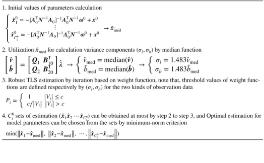
This presented algorithm is named LMS-RTLS, the algorithm is presented step by step in Table 1.

The efficiency of this algorithm is compared with that of traditional robust TLS (R-TLS) estimation using real data of mining area in the next section.

4 Experimental example and analysis

An experiment is carried out to verify the accuracy of data obtained in GNSS control sur- vey for mining area. Coordinates of control points obtained by the GNSS and known coor- dinates of points in the mining area are listed in Table 2.

Table 1 Iterative algorithm of LMS-RTLS 1. Initial values of parameters calculation

⎧⎪

⎨⎪

⎩

x̂⁰₁= −[A^T₀N⁻¹A0]⁻¹A^T₀N⁻¹𝝎⁰+x⁰

⋮ x̂⁰_C6

i

= −[A^T₀N⁻¹A0]⁻¹A^T₀N⁻¹𝝎⁰+x⁰ →x̂med

2. Utilization x̂med for calculation variance components ( 𝜎_l,𝜎_b ) by median function  

[v̂ b̂ ]

=

[Q₁ B^T₁₀ Q₂ B^T₂₀ ]

𝝀̂ →

{v̂_med= median(v)̂ b̂

med= median(b)̂ →

{𝜎_l=1.483v̂

med

𝜎_b=1.483b̂

med

3. Robust TLS estimation by iteration based on weight function, note that, threshold values of weight func- tions are defined respectively by ( 𝜎

l,𝜎

b ) for the two kinds of observation data  P

i=

{ 1 ||V

i||≤c

c∕||V

i|| ||V

i||>c 4. C⁶

i sets of estimation ( x̂₁x̂₂⋯x̂C⁶_i ) can be obtained at most by step 2 to step 3, and Optimal estimation for model parameters can be chosen from the sets by minimum-norm criterion

 min(‖‖x̂₁− ̂x_med‖‖,‖‖x̂₂−̂x_med‖‖, ⋯,‖‖‖x̂C⁶ i− ̂x_med‖‖‖)

Table 2 Results of checking planar coordinates of control points

For coordinates obtained by the GNSS, the coordinates of control point No. 1 are taken as true values while coordinates of other points are obtained by constraint estimation

Dot mark Known coordinates Coordinates by GNSS x₁ (m) y₁ (m) x₂ (m) y₂ (m)

1 3909.484 653.075 3909.484 653.075

2 3892.751 919.480 3892.883 919.342

3 4297.145 920.001 4297.131 920.133

Differences in distances and azimuths between coordinates from Table 2 are computed and listed in Table 3. The results of verification demonstrate that observation data of the mining area are more readily contaminated by gross error than observation data obtained for other conditions.

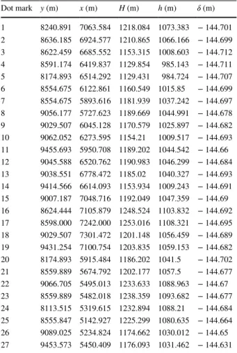
In the next part, observation data of the mining area are used to compare the proposed solution (LMS-RTLS) with traditional solutions. The observation data obtained by the GNSS and leveling measurements are listed in Table 4.

Table 3 Relative position differences of control points

Dot mark Known coordinates Coordinates by GNSS Relative difference Distance (m) Azimuth Distance (m) Azimuth Distance Azimuth

1–2 266.930 93°35′38.57″ 266.784 93°34′03.07″ 1/1828 1′35.50″

2–3 404.394 0°04′25.74″ 404.249 0° 06′43.55″ 1/2786 2′17.81″

Table 4 Observation data obtained by the GNSS and leveling measurements in the mining area

Dot mark y (m) x (m) H (m) h (m) 𝛿 (m) 1 8240.891 7063.584 1218.084 1073.383 − 144.701 2 8636.185 6924.577 1210.865 1066.166 − 144.699 3 8622.459 6685.552 1153.315 1008.603 − 144.712 4 8591.174 6419.837 1129.854 985.143 − 144.711 5 8174.893 6514.292 1129.431 984.724 − 144.707 6 8554.675 6122.861 1160.549 1015.85 − 144.699 7 8554.675 5893.616 1181.939 1037.242 − 144.697 8 9056.177 5727.623 1189.669 1044.991 − 144.678 9 9029.507 6045.128 1170.579 1025.897 − 144.682 10 9062.052 6273.595 1154.21 1009.517 − 144.693 11 9455.693 5950.708 1189.202 1044.542 − 144.66 12 9045.588 6520.762 1190.983 1046.299 − 144.684 13 9038.551 6778.472 1185.02 1040.327 − 144.693 14 9414.566 6614.093 1153.934 1009.243 − 144.691 15 9007.187 7048.716 1192.049 1047.359 − 144.69 16 8624.444 7105.879 1248.524 1103.832 − 144.692 17 8598.000 7242.000 1253.016 1108.321 − 144.695 18 9029.507 7301.472 1201.148 1056.459 − 144.689 19 9431.254 7100.754 1203.835 1059.153 − 144.682 20 8174.893 5915.484 1186.202 1041.5 − 144.702 21 8559.889 5674.792 1202.177 1057.5 − 144.677 22 9066.705 5495.013 1233.633 1088.963 − 144.67 23 8559.889 5482.018 1238.359 1093.682 − 144.677 24 8113.515 5319.615 1232.894 1088.21 − 144.684 25 8555.847 5142.927 1225.299 1080.635 − 144.664 26 9089.025 5234.824 1174.662 1030.012 − 144.65 27 9453.573 5450.409 1176.093 1031.462 − 144.631

Control points Nos. 3, 4, 6, 7, 9, 10, 12, and 13 are used to compute parameters of the fitting model using three algorithms. The distribution of control points is shown in Fig. 1.

The quantity of observation data for computation should be more than the quantity needed to obtain the variance of parameter estimation. The fitting model (2) requires six sets of observation data for computing parameters, and a maximum of eight sets of parameter estimation can be computed using the eight control points. Error of 1–3 m is introduced to coordinates of control points Nos. 4, 7, 10, and 13 while error of 1–2 m is introduced to the corresponding height anomalies to simulate gross error. Data are listed in Table 5 (where data with gross error are indicated in italics).

Control points for the computation of model parameters that have not been contami- nated with gross error are firstly used to compute parameters based on LS and TLS estimation. It is noted that the condition number of the normal matrix is 1.26 × 10²⁴, the normal equation is ill posed, and ridge estimation is used for regularization (Dongfang et al. 2016). Fitting residuals of control points based on LS and TLS algorithms (based Fig. 1 Distribution of control points

Table 5 Data of control points

with gross error Dot mark y (m) x (m) 𝛿 (m)

4 8593.374 6419.837 − 144.711

7 8554.675 5893.616 − 146.697

10 9062.052 6272.095 − 144.693

13 9038.551 6778.472 − 145.693

Table 6 Fitting residuals of

control points Dot mark LS (m) TLS (m) LS (g/m) TLS (g/m)

3 − 0.016 − 0.002 0.137 0.032

4 − 0.021 0.006 − 0.193 − 0.220

6 − 0.015 − 0.005 − 0.024 0.463

7 − 0.013 0.002 0.061 − 0.241

9 − 0.024 0.00005 − 0.013 0.218

10 0.001 0.0006 − 0.172 − 0.278

12 − 0.030 − 0.002 0.372 0.087

13 − 0.016 0.0009 − 0.212 0.076

on singular value decomposition, Golub and Van Loan 1980) are listed in Table 6, marked LS and TLS respectively. To compare with observation data that are free of gross error, control points of which some are contaminated with gross error (listed in Table 5) are used to compute parameters on the basis of LS and TLS estimation, which have 100 iterations. These results are also listed in Table 6, marked LSg and TLSg respectively.

Control points not used to compute model parameters are used to check the accuracy of the fitting model. The results are listed in Table 7.

Comparison with computation results obtained using control points that are free of gross error shows that the introduction of gross error into control points clearly affects the results of parameter estimation. To overcome the effect of gross error on parameter esti- mation, robust estimation is used for parameter estimation. Two algorithms—traditional Table 7 Accuracy of the fitting

model determined by check points

Dot mark LS (m) TLS (m) LS (g/m) TLS (g/m)

1 0.660 − 0.441 1.719 2.257

2 0.001 − 0.038 − 1.547 0.287

5 0.685 − 0.422 4.946 2.687

8 0.048 − 0.036 − 2.298 − 1.436

11 0.734 − 0.429 4.184 4.503

14 0.573 − 0.295 2.654 1.346

15 − 0.012 − 0.012 − 4.146 − 4.580

16 0.044 − 0.079 − 3.360 − 3.017

17 0.108 − 0.116 − 4.925 − 2.347

18 0.048 − 0.045 − 8.059 − 5.290

19 0.610 − 0.322 − 2.975 − 3.325

20 0.609 − 0.350 1.014 2.049

21 − 0.021 − 0.013 − 4.640 − 3.915

22 0.105 − 0.072 − 5.162 − 5.225

23 0.003 − 0.015 − 7.728 − 7.013

24 0.757 − 0.414 − 8.851 − 9.056

25 0.059 − 0.045 − 14.815 − 12.939

26 0.189 − 0.140 − 9.382 − 7.892

27 0.843 − 0.529 − 0.352 1.057

Table 8 Residual existing in observation data of the coefficient matrix

Dot mark x y xy x² y²

3 − 0.004 0.004 1.84−07 1.84E−07 −2.95E−07

4 0.024 − 0.025 − 1.13E−06 − 1.13E−06 1.80E−06

6 − 0.053 0.053 2.43E−06 2.43E−06 − 3.89E−06

7 0.027 − 0.027 − 1.23E−06 − 1.23E−06 1.97E−06

9 − 0.025 0.025 1.16E−06 1.16E−06 − 1.85E−06

10 0.031 − 0.031 − 1.43E−06 − 1.43E−06 2.28E−06

12 − 0.010 0.010 4.75E−07 4.75E−07 − 7.60E−07

13 − 0.009 0.009 4.29E−07 4.28E−07 − 6.85E−07

robust TLS estimation (R-TLS) and the proposed algorithm (LMS-RTLS)—are used for parameter estimation of the fitting model with 100 iterations, and the fitting residual in observation data of the coefficient matrix is listed in Table 8 (Schaffrin and Wieser 2008).

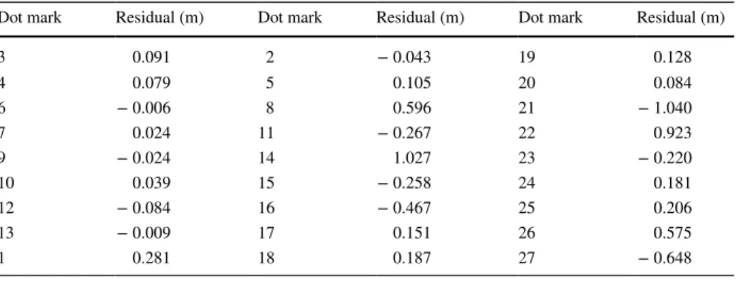
The variance component 𝜎₀ is 0.474 (computed by the proposed algorithm of Schaffrin and Wieser 2008). It is known that the residual estimation of elements in an observation Table 9 Fitting residuals of observation data obtained by LMS-RTLS

Dot mark Residual (m) Dot mark Residual (m) Dot mark Residual (m)

3 0.091 2 − 0.043 19 0.128

4 0.079 5 0.105 20 0.084

6 − 0.006 8 0.596 21 − 1.040

7 0.024 11 − 0.267 22 0.923

9 − 0.024 14 1.027 23 − 0.220

10 0.039 15 − 0.258 24 0.181

12 − 0.084 16 − 0.467 25 0.206

13 − 0.009 17 0.151 26 0.575

1 0.281 18 0.187 27 − 0.648

Fig. 2 Distribution of the fitting residual for control points

Fig. 3 Distribution of the fitting residual for check control points

vector and coefficient matrix (listed in Tables 7 and 8) is smaller than the variance com- ponent, and robust TLS estimation thus fails to optimally estimate model parameters. The reason why the residual estimation of observation data is smaller than the variance com- ponent has been explained in the literature (Xiaohua et al. 2011). To apply the proposed algorithm in the present study, the eight control points (Nos. 3, 4, 6, 7, 9, 10, 12, and 13) are separated into eight groups, with each group having seven control points. Applying the LMS-RTLS algorithm, the fitting residual of the eight control points and check control points is computed as listed in Table 9.

Figure 2 shows the distribution of fitting residuals for control points computed sepa- rately by LS estimation, R-TLS estimation, and LMS-RTLS estimation while Fig. 3 shows the distribution of fitting residuals for check control points.

Results reveal that traditional solutions fail in robust and robust estimation; i.e., the EIV model based on LMS regression is more efficient than traditional robust estimation when observation data have gross error. Observation data are more readily contaminated by gross error in a mining area than under usual conditions. The results show that gross error in the observation data obviously and adversely affects the final accuracy of the height anomaly fit- ting. Additionally, TLS estimation is less efficient than LS estimation when observation data have gross error while the fitting result based on TLS estimation is clearly more accurate than that based on LS estimation when observation data are free of gross error. Note that, because of unavoidable shortcomings, the traditional robust solution fails in estimation. Furthermore, the height anomaly fitting model is an ill-posed model, which obviously affects the fitting accuracy.

5 Conclusions

There is an extensive robust estimation problem in the field of geodesy. This paper mainly addresses robust TLS estimation for GNSS height anomaly fitting of mining area, which obviously has an EIV model. An analysis of traditional solutions reveals two obvious dis- advantages of current solutions, which are verified experimentally. To overcome the short- comings of traditional solutions for parameter estimation of an EIV model with outliers, a modified algorithm based on LMS regression was proposed. The proposed solution uses the median method to compute stable initial values and computes separate threshold values of the weight function for the coefficient matrix and observation vector. In an experiment, an iterative algorithm based on the proposed solution was demonstrated to be feasible and shown to obtain results that were more stable and accurate than traditional methods.

Additionally, its efficiency was compared with the efficiencies of traditional solutions. The experiment revealed that traditional robust TLS estimation has no clear advantage over LS estimation of mining area when observation data have gross error.

Acknowledgements The authors would like to thank the reviewers and the editor. This research was sup- ported by the National Natural Science Foundation of China (41601501; 41271135), Natural Science Found for Colleges and Universities of Jiangsu Province (16KJD420001) and Huaian Key Laboratory of Geo- graphic Information Technology and Applications (HAP201405).

References

Adcock RJ (1877) Note on the method of least squares. Analyst 4:183–184

Amiri-Simkooei AR (2013) Application of least squares variance component estimation to errors-in-varia- bles models. J Geodesy 87(10):935–944

Dongfang L, Jianjun Z, Yingchun S et al (2016) Construction method of regularization by singular value decomposition of design matrix. Acta Geod Cartogr Sin 45(8):883–889

Fang X (2015) Weighted total least-squares with constraints: a universal formula for geodetic symmetrical transformations. J Geodesy 89(5):459–469

Golub GH, Van Loan CF (1980) An analysis of the total least squares problem. SIAM J Number Anal 17:883–893

Heiskanen WA, Moritz H (1967) Physical geodesy. W H Freeman and Company, San Francisco Jiangwen Z (1989) Classic theory of errors and robust estimation. Acta Geod Cartogr Sin 18(2):115–120 Ling Y, Yunzhong S, Lizhi L (2011) Equivalent weight robust estimation method based on median param-

eter estimates. Acta Geod Cartogr Sin 40(1):28–32

Lu J, Chen Y, Li BF, Fang X (2014) Robust total least squares with reweighting iteration for three-dimen- sional similarity transformation. Surv Rev 46(334):28–36

Mahboub V (2012) On weighted total least-squares for geodetic transformation. J Geodesy 86(5):359–367 Mahboub V (2014) Variance component estimation in errors-in-variables models and a rigorous total least-

squares approach. Stud Geophys Geod 58(1):17–40

Mahboub V, Amiri-Simkooei AR, Sharifi MA (2013) Iteratively reweighted total least squares: a robust esti- mation in error-in-variables models. Surv Rev 45(329):92–99

Neitzel F (2010) Generalization of total least-squares on example of unweighted and weighted 2D similarity transformation. J Geodesy 84(12):751–762

Pan G, Zhou Y, Sun H et al (2015) Linear observation based total least squares. Surv Rev 47(340):18–27 Peiliang X, Liu J, Shi C (2012) Total least squares adjustment in partial errors- in-variables models: algo-

rithm and statistical analysis. J Geodesy 86(8):661–675 Peter JH (1981) Robust statistics. Wiley, Hoboken

Rousseeuw P, Wagner J (1994) Robust regression with a distribution intercept using least median of squares.

Comput Stat Data Anal 17:65–76

Schaffrin B (2006) A note on constrained total least-squares estimation. Linear Algebra Appl 417:245–258 Schaffrin B, Felus YA (2008) On the multivariate total least-squares approach to empirical coordinate trans-

formations: three algorithms. J Geodesy 82(6):373–383

Schaffrin B, Felus YA (2009) An algorithmic approach to the total least-squares problem with linear and quadratic constraints. Stud Geophys Geod 53:1–16

Schaffrin B, Uzun S (2011) Error-in-variables for mobile mapping algorithms in the presence of outliers.

Arch Photogramm Cartogr Remote Sens 22:377–387

Schaffrin B, Wieser A (2008) On weighted total least-squares adjustment for linear regression. J Geodesy 82(7):415–421

Schaffrin B, Lee I, Choi Y et al (2006) Total least squares (TLS) for geodetic straight-line and plane adjust- ment. Bull Geod Sc Aff 65:141–168

Shen Y, Li B, Chen Y (2011) An iterative solution of weighted total least-squares adjustment. J Geodesy 85(4):229–238

Tao Y, Gao J, Yao Y (2014) TLS algorithm for GPS height fitting based on robust estimation. Surv Rev 46(336):184–188

Xiaohua T, Yanmin J, Lingyun L (2011) An improved weighted total least squares method with applications in linear fitting and coordinate transformation. J Surv Eng 137(4):120–128

Xuming G, Jicang W (2012) Generalized regularization to ill-posed total least squares problem. Acta Geod Cartogr Sin 41(3):372–377

Xunqiang G, Zhilin L (2014) A robust weighted total least squares method. Acta Geod Cartogr Sin 43(9):888–894

Yang Y (1999) Robust estimation of geodetic datum transformation. J Geodesy 73(5):268–274