Origins of oscillatory dynamics in the model of reactive oxygen species in the rhizosphere
Stevan Ma´ceˇsi´c,1,a)Agota T´´ oth,1 and Dezs˝o Horv´ath2,b)
1)Department of Physical Chemistry and Materials Science, University of Szeged, Rerrich B´ela t´er 1, 6720 Szeged, Hungary
2)Department of Applied and Environmental Chemistry, University of Szeged, Rerrich B´ela t´er 1, 6720 Szeged, Hungary
(Dated: 21 September 2021)
Oscillatory processes are essential for normal functioning and survival of biological systems and reactive oxygen species have a prominent role in many of them. A mechanism representing the dynamics of these species in the rhizosphere is analyzed using stoichiometric network analysis with the aim to determine its capabilities to simulate various dynamical states including oscillations. A detailed analysis has shown that unstable steady states result from four destabilizing feedback cycles, among which the cycle involving hydroquinone, an electron acceptor and its semi-reduced form, is the dominant one responsible for the existence of saddle-node and Andronov-Hopf bifurcations. This requires higher steady-state concentration for the reduced electron acceptor compared to that of the remaining species, where the level of oxygen steady-state concentration determines whether Andronov-Hopf or saddle-node bifurcation will occur.
I. INTRODUCTION
Various systems in chemistry and biology1 are known for the ability of self-organization when found under conditions far from equilibrium. As a result of this, they are capable of exhibiting different types of temporal and spatio-temporal phenomena such as bistability2–4, oscillations5–8, chaos9,10, reaction-diffusion fronts7,11–13, etc. Oscillatory dynamics is especially important for biological systems where many processes are character- ized by periodic behavior with periods ranging from seconds (calcium oscillations)14,15, minutes (glycolytic oscillations)16,17 to the hours (circadian clock)18, days and months (hormonal oscillations)19–21. For survival, biological systems have to adapt to sudden and very often periodical changes in their surroundings. Hence many bi- ological processes are also periodic, therefore understand- ing their mechanisms is of great importance.
Reactive oxygen species (ROS) are closely related to the oscillatory dynamics of biological processes.22 ROS are byproducts of biochemical reactions that involve O2 and produce energy vital for the normal functioning of plants and other aerobic organisms. ROS are formed as a result of the ability of O2 to easily accept electrons because of the two unpaired electrons in the outermost orbital. The presence of ROS can have negative and positive impacts on the biological systems depending on the level of their concentrations. ROS have an impor- tant role as signaling molecules in plants when they are present in low concentrations23,24, but high ROS concen- trations can make irreparable damage due to their high reactivity which allows them to oxidize almost all biolog- ical molecules, including DNA, proteins and lipids25–28.
a)Also at Faculty of Physical Chemistry, University of Belgrade, Studentski Trg 12, 11158 Belgrade, Serbia
b)Electronic mail: horvathd@chem.u-szeged.hu
Taran et al.29 conducted a series of experiments to investigate ROS dynamics in the rhizosphere, the nar- row zone of soil along plant root surfaces. In this area, ROS are produced as a result of various redox pro- cesses. A model system was designed mimicking the ri- zosphere in which they focused on reactions between two redox pairs, 2,6-dimethoxybenzoquinone/hydroquinone and methylene blue/leuco-methylene blue, in the pres- ence of both sodium borohydride, as a reducing agent, and oxygen. Experiments were carried out both in well- stirred reactors and in thin layers of solution where dif- fusion is present. They have found that the system can display autocatalytic behavior and produce reaction- diffusion fronts. Based on these results they proposed a reaction network that resembles the mechanism of the reaction between methylene blue and sulfide ion, which is known to produce oscillations.30
In this work we carry out a thorough investigation of the network that is the core of their proposed model to analyze its full capacity to produce oscillatory dynamics and to determine the conditions required for its existence.
By performing stability analysis using stoichiometric net- work analysis (SNA)31–34, we will show that destabilizing feedback cycles can be detected and we will identify the conditions essential for the emergence of bistability and oscillations.
II. MODEL AND METHODS A. Model
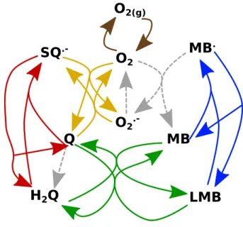
The model, defined by reactions in eqn (R1–R9), is represented in Fig. 1. Quinone is reduced by sodium borohydride in the first step (R1). Synproportionation of hydroquinone and quinone takes place according to eqn (R2) forming the semiquinone radical that can react with oxygen producing a reactive oxygen species in eqn hor’s peer reviewed, accepted manuscript. However, the online version of record will be different from this version once it has been copyedited and typeset. PLEASE CITE THIS ARTICLE AS DOI:10.1063/5.0062139
(R3). In a similar fashion, synproportionation of the sec- ond redox pair, methylene blue and leucomethylene blue in this specific case, in eqn (R4) gives a reactive inter- mediate MB·radical, which reacts with dissolved oxygen in eqn (R5) producing a reactive oxygen species. The coupling between the methylene blue and hydroquinone systems is via a two-electron redox process in eqn (R6).
The disproportionation of ROS to oxygen and hydrogen peroxide is according to in eqn (R7). The dissolution of oxygen follows eqn (R8), while the decomposition of sodium borohydride eqn (R9).
O
2O
2.-Q
H
2Q SQ
.-MB
LMB MB
.O
2(g)FIG. 1. Schematic representation of the model (R1)–(R9) and the corresponding reaction rates presented in Table I.
The colored solid lines show the reversible reactions only.
NaBH4+ Q→borates + H2Q (R1) H2Q + Q⇋2SQ·−+ 2H+ (R2) SQ·−+ O2⇋Q + O·−2 (R3)
MB + LMB⇋2MB·+ 2H+ (R4)
MB·+ O2→MB + O·−2 (R5)
MB + H2Q⇋LMB + Q (R6)
2O·−2 + 2H+⇋2HO2→O2+ H2O2 (R7)
O2(g)⇋O2 (R8)
NaBH4→borates + H2 (R9) In this complex reaction network the concentrations of eight species, 2,6-dimethoxybenzoquinone (Q), hy- droquinone (H2Q), semiquinone (SQ·–), oxygen (O2), superoxide radical (O·2–), methylene-blue (MB), leuco- methylene blue (LMB) and semi-reduced methylene blue (MB·), comprise the dynamical variables. The main re- actant, sodium borohydride, is applied in a concentra- tion considerably higher than the concentrations of other
TABLE I. Rate equations of the network in Fig. 1. with rate coefficients allowing oscillatory dynamics.
r1=k′1[Q] k′1= 1.00×10⁻²s−1 r2=k2[H2Q][Q] k2= 1.00×10³ M−1s−1 r−2=k−2[SQ·−]2 k−2= 1.00×10⁸M−1s−1 r3=k3[SQ·−][O2] k3= 7.35×10⁴ M−1s−1 r−3=k−3[Q][O·−2 ] k−3= 4.93×10³M−1s−1 r4=k4[MB][LMB] k4= 6.47×10³ M−1s−1 r−4=k−4[MB·]2 k−4= 1.00×10⁸M−1s−1 r5=k5[MB·][O2] k5= 1.38×10⁵ M−1s−1 r6=k6[MB][H2Q] k6= 2.85×10⁴ M−1s−1 r−6=k−6[LMB][Q] k−6= 1.25×10²M−1s−1 r7=k7[O·−2 ]2 k7= 1.80×10⁴ M−1s−1 r8=k′8 k′8= 2.25×10⁻⁷M s−1 r−8=k−8[O2] k−8= 1.00×10⁻³ s−1
species and therefore it is considered as a pool chemical with a constant concentration. Even though we drive the reduction process with the excess of borohydride, in the presence of O2 in the solution, ROS are formed by two redox cycles that are mutually coupled.
In our analysis we consider pseudo steady states with borohydride in great excess, therefore, without the loss of generality, reaction (R9) is omitted from the model. This condition is important because the hydrolysis of sodium borohydride itself can follow oscillatory dynamics in a continuously stirred tank reactor35,36. Here we focus on the dynamics of the redox couples which requires the re- ducing agent in great excess. The concentration of H+ is considered to be constant at the level of pH = 8.5 and it is included in the values of the appropriate rate constants.29 The constant pH can only be maintained with a buffer system that is chemically inert with re- spect to reactions (R1)-(R9), which is indeed the case in the rhizosphere. Reaction (R7) involves a fast pre- equilibrium that transforms O·–2 and H+ directly into O2 and H2O2. The oxygen level in the air is considered constant, hence a constant rate for the dissolution is set in accordance with the solubility of molecular oxygen.
One set of parameters used in the simulations is listed in Table I.
B. Methods
Numerical simulations and stoichiometric network analysis were performed using the program Octave, where the solutions of algebraic equations provide the steady states and the stability if needed as a function of the parameters. For solving the ordinary differential equations in order to describe the temporal evolution of the species,LSODE function with a backward differentia- tion formula as the integration method was utilized with the absolute tolerance set to 10−14.
hor’s peer reviewed, accepted manuscript. However, the online version of record will be different from this version once it has been copyedited and typeset. PLEASE CITE THIS ARTICLE AS DOI:10.1063/5.0062139
III. RESULTS AND DISCUSSION 1. Stoichiometric network analysis
The essence of stoichiometric network analysis (SNA) is the handling of reaction rates as variables instead of the concentrations used in the classical approach.37–39 This facilitates the selection of reactions that are essential in the appearance of instabilities and allows the reduction in the number of parameters. Hence with this powerful method, we can identify the sub-networks that carry the instability that can lead to oscillations.
In the first step, the steady-state equations are ex- pressed as a linear combination of the reaction rates rss
as
dc
dt =f =S rss= 0 (1) where Srepresents the stoichiometric matrix of the dy- namical variables. In our model the rank of the stoi- chiometric matrix S is 6, while there are 8 dynamical variables. This is a direct consequence of the two conser- vation constraints from the stoichiometry of quinone and the methylene blue species as
[Q]+[H2Q]+[SQ·−] = [Q]0+[H2Q]0+[SQ·−]0=QT (2) [MB]+[LMB]+[MB·] = [MB]0+[LMB]0+[MB·]0=M BT
(3) where T subscript refers to the total amount of quinone and methylene blue and 0 subscript to the initial values.
The solutions of eqn (1)40–42 for the rates yields the matrix of extreme currentsE43
E=
E1 E2 E3 E4 E5 E6 E7 E8
0 0 0 0 0 1 0 1 R1
1 0 0 0 0 1 0 0 R2
1 0 0 0 0 0 1 0 R−2
0 1 0 0 0 2 0 0 R3
0 1 0 0 0 0 2 0 R−3
0 0 1 0 0 0 1 1 R4
0 0 1 0 0 0 0 0 R−4
0 0 0 0 0 0 2 2 R5
0 0 0 1 0 0 1 1 R6
0 0 0 1 0 0 0 0 R−6
0 0 0 0 0 1 0 1 R7
0 0 0 0 1 1 0 1 R8
0 0 0 0 1 0 0 0 R−8
(4)
In matrixEeach column represents one reaction route in the steady-state (also termed a sub-network capable to achieve a steady state), while each row contains the contribution of a chemical reaction to the relevant sub- network. All elements of matrixEare non-negative num- bers and each direction in the reversible reactions is con- sidered as a separate reaction. In this way the governing equations at the steady state ri,ss can be expressed as
positive linear combination of the columns of matrix E by introducing new parameters, i.e., current ratesj and by using the main relation of SNA rss = E j. Current ratesjiare non-negative numbers that represent the con- tribution of each reaction routeEi to the corresponding reaction rate in a steady state.
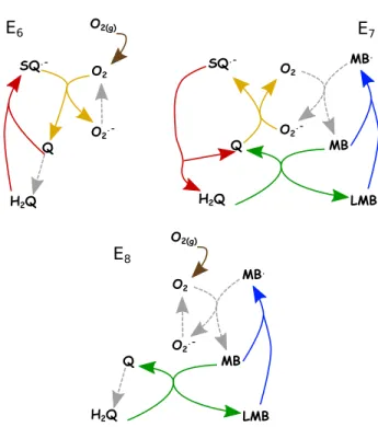
Matrix E of our model has 8 columns, i.e., 8 steady- state reaction routes. Among them 5 are equilibrium ones consisting of only reversible reactions with no net reaction: E1(R2/R−2), E2(R3/R−3), E3(R4/R−4), E4(R6/R−6) andE5(R8/R−8). Alone, they cannot pro- duce instabilities, but in combination with other reac- tion routes they can significantly contribute to the rise of instabilities. Reaction routeE6(R1, R2, R3, R7, R8) (see Fig. 2) includes only reactions which describe Q redox cycle coupled with self-oxidation of O2. Reaction routes E7(R−2, R−3, R4, R5, R6) andE8(R1, R4, R5, R6, R7, R8) (see Fig. 2) are minimal sub-networks that include cou- pling between Q and MB redox cycles. In the case of sub-network E7, this coupling is done in two ways to maintain the steady-state: directly through reactionR6
and indirectly by species O2and O·–2 . Contrarily, in sub- networkE8coupling exists only directly through reaction R6, while O2 maintains the MB redox cycle. Reaction routeE7 has no net reaction, whileE6andE8share the common net reaction of
NaBH4+ O2(g)→borates + H2O2 (R10)
O2
O2.-
Q
H2Q SQ.-
O2(g)
O2
O2.-
Q
H2Q SQ.-
MB
LMB MB.
O2
O2.-
Q
H2Q
MB
LMB MB. O2(g)
E6 E7
E8
FIG. 2. Schematic representation of reaction routes: E6,E7, E8
Using the equation rss = E j, the reaction rates in the steady states can be expressed as the following linear hor’s peer reviewed, accepted manuscript. However, the online version of record will be different from this version once it has been copyedited and typeset. PLEASE CITE THIS ARTICLE AS DOI:10.1063/5.0062139
combinations ofji
r1,ss=j6+j8
r2,ss=j1+j6 r−2,ss=j1+j7
r3,ss=j2+ 2j6 r−3,ss=j2+ 2j7
r4,ss=j3+j7+j8 r−4,ss=j3
r5,ss= 2j7+ 2j8
r6,ss=j4+j7+j8 r−6,ss=j4
r7,ss=j6+j8
r8,ss=j5+j6+j8 r−8,ss=j5
(5)
The stability of the steady-state can be determined by calculating the eigenvalues of the Jacobian matrix (M) that contains the∂fi/∂cj terms evaluated at the steady state. In SNA31,43,44it is expressed as a function of rates according to
M(j,h) =Sdiag(E j)KTdiag(h) (6) whereK is the matrix of reaction orders, andh= 1/css
represents the vector of the reciprocal steady state con- centrations. Equation (6) results from elementary steps in the model, for which ∂ri/∂cj = Ki,jri/cj is valid.
When one or more eigenvalues have positive real parts, the steady state is unstable, otherwise it is stable.
An efficient way to determine the stability is to use the so-called Hurwitz determinants or theα-approximation, according to which an eigenvalue with a positive real part occurs when some coefficientαiof the characteristic poly- nomial is negative.44,45 Condition for the appearance of Andronov–Hopf (AH) bifurcation is that the Hurwitz de- terminant ∆n−1 = 045, while the condition for the ap- pearance of saddle-node (SN) bifurcation is that αn = 044, where n is the number of linearly independent dy- namical variables.
In the case of complex models the search for conditions supporting instability becomes simpler if we inspect the matrix of current ratesV(j), defined as thej-dependent part of eqn (6) according to
V(j) =−Sdiag(E j)KT (7) Instability can now be detected to a good approximation31 by the existence of at least one negative diagonal minor inV(j).
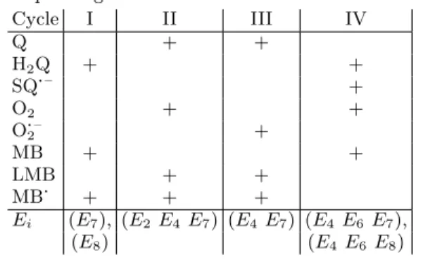
By analyzing the negative terms, in α3–α6 and the diagonal minors ofV(j), we have identified the origin of possible instabilities: four distinct destabilizing feedback cycles (I, II, III, and IV) are responsible for the existence of unstable steady states with the corresponding dynamic variables as summarized in Table II.
A. Dominant destabilizing feedback cycle
Although all four cycles can, in principle, produce un- stable steady states, the simplest cycle with the most flex- ible instability conditions is the most important because this is expected to be the experimentally most accessible.
TABLE II. Destabilizing cycles with their relevant species and the corresponding minimal sub-networks
Cycle I II III IV
Q + +
H2Q + +
SQ·– +
O2 + +
O·–2 +
MB + +
LMB + +
MB· + + +
Ei (E7), (E2E4E7) (E4 E7) (E4 E6 E7),
(E8) (E4 E6 E8)
To identify this dominant cycle, we have compared them in terms of the numbers of interacting species and the size of the minimal sub-network required for their existence (see Table II).
O2
O2.-
Q
H2Q SQ.-
MB
LMB MB.
O2
O2.-
Q
H2Q SQ.-
MB
LMB MB.
O2
O2.-
Q
H2Q SQ.-
MB
LMB MB. O2(g)
Cycle II Cycle III
Cycle IV
FIG. 3. Schematic representation of destabilizing cycles II, III and IV. Diagrams represents minimal set of columns of E required for cycle to be unstable; Cycle II (E2E4E7), Cycle III (E4E7), Cycle IV (E4E6E8)
Analysis has shown that cycle I is the dominant be- cause this cycle is composed of only three interacting species, unlike the rest. Furthermore, cycles II–IV in- clude at least one species from cycle I. For cycle I to become unstable, it is necessary to include only a sub- network represented by extreme currents ofE7orE8. For cycles II–IV, summarized in Fig. 3, to become unstable, two or more columns of matrixE have to be combined but all unstable combinations containE7 or E8. Since extreme currents ofE7 and E8 are present in all desta- bilizing cycles, the coupling between Q and MB redox hor’s peer reviewed, accepted manuscript. However, the online version of record will be different from this version once it has been copyedited and typeset. PLEASE CITE THIS ARTICLE AS DOI:10.1063/5.0062139
cycles is crucial for the appearance of instabilities. This conclusion is also supported by the fact that sub-network E6, which incorporates only redox cycle related to Q in the presence of O2, cannot become unstable unlessE7or E8 is present.
Two types of instability are identified within the net- work: saddle-node bifurcation where bistability is sought and Andronov–Hopf-bifurcation which represents the birth of oscillatory dynamics. These instabilities are ad- dressed in the next section.
B. Derivation of the conditions for Andronov–Hopf and saddle-node bifurcations
The large number of parameters (j1–j8 and h1–h8) that determine the stability of the model complicates the derivation of the exact conditions for bifurcations, there- fore the analysis has to be conducted in several steps.
In the first step, conditions under which cycle I becomes unstable is determined by analyzing the negative diago- nal minor of matrix V(j) of cycle I. This results in the inequality
(j1+j6) [2j3j4+ (j3+j4)J7,8]< J7,8(j3+J7,8)(j4+J7,8) (8) where J7,8 =j7+j8. Parametersj1 andj6 can only be found on the left side of this inequality and therefore they represent the main stabilizing terms. Contrarily,J7,8 is essential for the existence of instabilities and therefore the sum ofj7 and j8 is the main destabilizing term. In- equality (8) can be satisfied for various current rates, but setting all ji parameters to have the same value is the most suitable choice for several reasons. Firstly, when all current rates are equal, cycles II–IV are stable. Sec- ondly, this choice leads to a reduction in the number of parameters: there is only one current rate assigned as j0. Moreover, approximate analytical expressions for the steady-state concentrations as a function of rate con- stants can be calculated from eqn (5). Lastly, setting j1–j8 to have the same value asj0leads to simplification in the expressions forα3–α6 (all of them still have neg- ative terms) which allows us to derive conditions for the appearance of AH and SN bifurcations.
For SN bifurcation to emerge, it is necessary that α6 = 0. By calculating α6 and solving for h7 condi- tions (A1) and (A2) listed in Appendix A are derived.
Although O2 has to be present in the system for SN bi- furcation to occur, its steady-state concentration does not determine the condition for appearance of SN bifur- cation directly, as seen from eqn (A1) in Appendix A.
Condition for SN bifurcation is determined by delicate balances between concentrations of Q and MB species.
Condition (A2) in Appendix A ensures that only non- negative values of h7 are considered and it also shows that the critical value of h2 is determined only by the values ofh1 andh3, i.e., by the total amount of quinone in the system. From eqn (A2) it follows that h2 has to
be greater thanh1 and h3. Since h1, h2, and h3 corre- spond to the reciprocal steady-state concentrations of Q, H2Q and SQ–, respectively, for SN bifurcation to take place the steady-state concentration of H2Q has to be low compared to that of Q and SQ– according to
[H2Q]ss < 5
182[SQ·−]ss+ 54
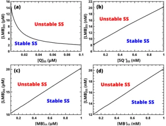
182[Q]ss , (9) the transformed form of eqn (A2). Analysis of eqn (A1) also reveals thath7has to be less thanh6andh8. Seeing thath6,h7, andh8 represent the reciprocal steady-state concentrations of MB, LMB, and MB·, respectively, SN bifurcation will appear when LMB steady-state concen- tration is greater than that of MB and MB·. By using eqn (A2) in Appendix A, it is possible to determine the position of SN bifurcation as a function of these con- centrations, as shown in Fig. 4. For instability to arise the methylene blue redox system has to be in its reduced state with LMB dominating over the other oxidized forms in the steady state (see Figs. 4(c,d)). Comparison of these two figures also reveals that the reactive MB· rad- ical is expected to be present in concentrations signifi- cantly smaller than the others in accordance with chemi- cal intuition. Large [LMB]/[Q] ratio favors stable steady state under pool conditions, therefore an increase in the concentration of Q destabilizes the steady state while the concentration of the reactive semiquinone radical remains small (see Figs. 4(a,b)).
[LMB]SS (μM)
10 15 20
[MB]SS (μM)
0.2 0.4 0.6 0.8 1
Unstable SS
Stable SS (c)
[LMB]SS (nM)
12 14 16 18 20
[MB.]SS (nM)
0.2 0.4 0.6 0.8 1
Unstable SS
Stable SS (d)
[LMB]SS (nM)
6 8 10 12 14 16 18 20 22
[SQ.-]SS (nM)
0.2 0.4 0.6 0.8 1
Unstable SS
Stable SS (b)
[LMB]SS (μM)
0 2 4 6 8 10 12 14 16
[Q]SS (μM)
0.02 0.04 0.06 0.08 0.1
Unstable SS
Stable SS (a)
FIG. 4. Location of saddle-node bifurcation in the concen- tration space with the value ofh2 set to be twice the critical value defined by eqn (A2) in Appendix A.
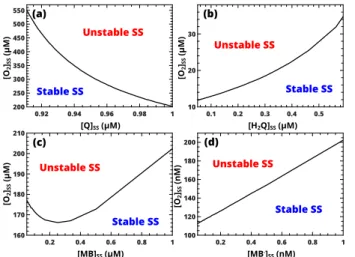
For the emergence of Andronov–Hopf bifurcation con- ditions (B1) and (B2), displayed in Appendix B, are de- rived from coefficientα5. Inequality (B1) is an approx- imation of the exact condition for the emergence of AH bifurcation but it has proved to be very reliable. The values ofh4and h7, i.e., the steady-state concentrations of O2and LMB, are found to be crucial. Condition (B2) have to be satisfied in order forh4 to have non-negative hor’s peer reviewed, accepted manuscript. However, the online version of record will be different from this version once it has been copyedited and typeset. PLEASE CITE THIS ARTICLE AS DOI:10.1063/5.0062139
values. By using eqn (B1), the position of AH bifurcation as a function ofh4 and h1, h2, h6 andh8 are examined for the required lower value of h7, i.e., higher concen- tration of LMB. Figures 5(a,b) show that the hydro- quinone/quinone system has to be in the oxidized state because [Q]ss >[H2Q]ss is needed for the instability to arise. Low concentration of MB also favors the instabil- ity (see Fig. 5(c)), while the reactive MB· remains in low concentration as expected for chemically realistic condi- tions (Fig. 5(d)).
[O2]SS (μM)
200 250 300 350 400 450 500 550
[Q]SS (μM)
0.92 0.94 0.96 0.98 1
Unstable SS
Stable SS (a)
[O2]SS (μM)
10 20 30
[H2Q]SS (μM)
0.1 0.2 0.3 0.4 0.5
Unstable SS
Stable SS (b)
[O2]SS (nM)
100 120 140 160 180 200
[MB.]SS (nM)
0.2 0.4 0.6 0.8 1
Stable SS Unstable SS (d)
[O2]SS (μM)
160 170 180 190 200 210
[MB]SS (μM)
0.2 0.4 0.6 0.8 1
Unstable SS
Stable SS (c)
FIG. 5. Location of Andronov–Hopf bifurcation in the con- centration space with the value ofh7set to be one fifth of the critical value defined by eqn (B2) in Appendix B.
C. Numerical bifurcation analysis
The conditions for AH and SN bifurcations discussed in the previous section have proved to be very accurate but they are the functions of numerous hi parameters.
Therefore, an additional investigation has been carried out in order to further confirm their validity and more importantly to test the significance of parameters for the emergence of AH and SN bifurcations. The numerical bifurcation analysis is performed by setting the values of j0 and h1−h8 to 1, then one or a combination of severalhi parameters are varied while all other are kept constant. In each step, selectedhi parameters are given the same value, the Hurwitz determinants are numeri- cally calculated, and the number of sign changes in the Routh-Hurwitz (RH) array are evaluated. In this way, the parameters important for the emergence of AH and SN bifurcations can be detected.
There are two essential combinations (h1,h7) and (h4, h7) that lead to the appearance of AH and SN bifurca- tions. All of them include h7, which suggests that ap- propriate steady-state concentration of LMB is essential for the emergence of unstable steady states. On the one hand, the decrease in h1 and h7 leads to the appear- ance of a single sign change in the Routh–Hurwitz array,
corresponding to the loss of stability via saddle-node bi- furcation. This is in accordance with the phase diagram in Fig. 4(a), where high steady-state concentrations of LMB and Q favor instability and confirm the conditions in eqn (A1)–(A2) of Appendix A. On the other hand, upon decreasing the (h4, h7) pair, a double sign change in the Routh–Hurwitz array occurs, indicating the loss of stability via Andronov–Hopf bifurcation. This means that high steady-state concentrations of LMB and O2are essential for the existence of oscillatory dynamics, which is also in agreement with the conditions in eqn (B1)–(B2) of Appendix B and further confirms the validity of eqn (A1)–(B2).
Up to this point, sodium borohydride is considered as a pool chemical with constant concentration. When we inspect the stability of the steady state as a func- tion of borohydride concentration, we find stable steady states at low concentration, however upon increasing the amount of borohydride, a bistable region bounded by saddle-node bifurcations (Fig. 6) or an oscillatory re- gion between Andronov–Hopf bifurcations (Fig. 7) can be found, depending on the parameters. Greater reducing agent concentrations are again characterized with stable steady states.
[MB]ss (μM)
0.1 1 10
[NaBH4]0 (M)
0.016 0.018 0.02 0.022 0.024 0.026 0.028
FIG. 6. Bistable region bounded by oxidized and reduced states as the sodium borohydride initial concentration is in- creased.
Considering that oxygen is also present in the system, the delicate balance between the oxydizing power of re- active oxygen species and the reducing power of boro- hydride can lead to the instability giving rise to bista- bility or oscillations. At low borohydride concentration, oxidation driven by ROS dominates, oppositely to high concentration where the fast reduction, both of which are present in reaction routes E6 and E8. These routes themselves cannot destabilize the steady state, for that E4 is needed in cycles II–IV, i.e. the coupling between the two redox systems, the quinone and the methylene blue in this particular model.
In a closed system with initial conditions matching the bistable region in the corresponding pool chemical system, reaction paths with fast and slow time scales representing an autocatalytic burst are feasible. With parameters placing the initial conditions in the range be- hor’s peer reviewed, accepted manuscript. However, the online version of record will be different from this version once it has been copyedited and typeset. PLEASE CITE THIS ARTICLE AS DOI:10.1063/5.0062139
[MB]ss (μM) 1 10
[NaBH4]0 (M)
0.04 0.05 0.06 0.07 0.08
FIG. 7. Two Andronov–Hopf bifurcations borders the region with unstable steady state that allow oscillations for a range of sodium borohydride initial concentration.
tween the Andronov–Hopf bifurcations, transient oscilla- tion can be achieved as shown in Fig. 8.
The original parameters used by Taran et al.29 do not comprise conditions in the vicinity of an Andronov–
Hopf bifurcation, no oscillations have been observed with them, therefore a systematic search within the parame- ter space is required to locate the desired behavior. One
[MB] (μM)
0 5 10 15 20 25 30 35
time (s)
0 10000 20000 30000 40000 50000
[Q] (μM)
10 12 14 16 18 20 22 24 26
0 10000 20000 30000 40000 50000
FIG. 8. Numerical simulation obtained with adjusted pa- rameters presented in Table I under batch conditions; Ini- tial conditions used in simulation: [NaBH4]0 = 5×10⁻²M, [Q]0= 2.58×10⁻⁵M, [MB]0= 4.10×10⁻⁵M. Initial concen- trations of remaining species were set to 0.
method to find the required parameter set is to fix allji
current rates to the same value of j0, which results in a simplified version of eqn (5). Using the relation between ri,ss and j0, analytical expressions for the steady-state
concentrations as functions of reaction rates ki can be derived. There are 13 relations in eqn (C1) of Appendix C that need to be satisfied but only 8 species and one j0parameter, therefore four rate constants are expressed as a function of the remaining. The value ofj0 is deter- mined only by the value ofk8 which represents the rate at which O2 enters the system. Since j0 is involved in all steady-state relations, this rate governs the dynamics which is in agreement with the results of stability and bifurcation analysis, since it appears in bothE6andE8. Detailed investigation has shown that the condition in eqn (B1) cannot be satisfied by changing only the re- actant concentrations in the parameter set of Taran et al.29 In other words, modified rate constants are neces- sary, which would require the change of reducing agent, electron acceptor or even a different hydroquinone may be needed for the experimental realization. One set of ad- justed rate constants that match eqn (B1) is presented in Table I. During the parameter search we have fixed the rate constant of (R7) because the ROS dynamics associ- ated with it does not change. The general outcome can be summarized as the following. The values of k3 and k−3 have to be reduced, however the relation k3 > k−3
can be preserved in accordance with the original set of values. For oscillatory dynamics steady-states with the electron acceptor in its reduced state, i.e. high LMB con- centrations, are needed, therefore the values of k6 and k−6have been changed significantly such that the former has become greater. Direct numerical simulation carried out with one set of adjusted rate constants under batch conditions produces temporal oscillation with appropri- ate initial conditions (see Fig. 8). Although these rate constants are chemically realistic, for constructing a spe- cific experiment to observe this oscillatory dynamics, a different electron acceptor has to be selected instead of methylene blue where the equilibrium constant between the redox pairs match the necessary conditions.
IV. CONCLUSION
Detailed analysis of the model describing the dynamics of ROS in the rhizosphere has been conducted to explore its dynamical properties. Stability analysis has proved the existence of Andronov–Hopf and saddle-node bifur- cations under appropriate conditions. Four destabilizing feedback loops govern the dynamics. The comprehen- sive analysis has also shown that the cycle involving hy- droquinone (H2Q), the electron acceptor (MB) and its semi-reduced form(MB·) itself is dominant because it is responsible for the emergence of bifurcations. The condi- tions for the appearance of bifurcations are also derived and their validity has been corroborated by numerical analysis.
We have identified that higher steady-state concentra- tions of the reduced electron acceptor (LMB) are required for obtaining unstable steady states. The type of insta- bilities are then determined by the steady-state concen- hor’s peer reviewed, accepted manuscript. However, the online version of record will be different from this version once it has been copyedited and typeset. PLEASE CITE THIS ARTICLE AS DOI:10.1063/5.0062139
tration of the dissolved oxygen: at low concentrations saddle-node bifurcations may emerge, while high steady- state concentration is required for oscillatory dynamics.
In both cases, preserving the delicate balance between the hydroquinon/quinone system and the electron accep- tor is essential.
By selecting methylene blue as the electron acceptor to couple with the hydroquinone/quinone system and sodium borohydride as the reducing agent in excess,29 bursts can be produced that lead to reaction-diffusion fronts with the experimentally accessible parameter set.
In the rizosphere the ROS-hydroquinone reaction net- work, as we have shown, can have the capability of yield- ing oscillatory dynamics that can drive biologically im- portant processes depending on the electron acceptor and the reducing species. Nonlinear responses, such as auto- catalytic bursts and oscillations, can then provide the regulatory signals that are essential in living systems.
DATA AVAILABILITY STATEMENT
The data that support the findings of this study are available from the corresponding author upon reasonable request.
ACKNOWLEDGMENTS
This work was supported by the National Research, Development and Innovation Office (K119795) and GINOP-2.3.2-15-2016-00013 project. S.M. acknowledges the support by the Ministry of Education, Sciences and Technology of the Republic of Serbia (172015 and 451- 03-9/2021-14/200146).
Appendix A: Condition for saddle-node bifurcation
Regarding the reciprocal steady-state concentrations (hi) in the stoichiometric network analysis, the inequality h7≤ 3h6h8(5h1h2−182h1h3+ 54h2h3)
540H126+ 72h3h6(h2+ 17h1) + 607H128+ 734H138+ 258H238
(A1) withHijk=hihjhkmust be satisfied for saddle-node bifurcation to occur, where the right hand side must be positive.
This results in the additional requirement of
h2> 182h1h3
5h1+ 54h3
. (A2)
Appendix B: Condition for Andronov–Hopf bifurcation
Regarding the reciprocal steady-state concentrations (hi) in the stoichiometric network analysis, the inequality h4< −2h5(3H1267−2H1268+ 6H1367+ 5H1278+ 6H1378−4H2368+ 4H2378)
h5(6H126+ 5H127+ 8H136+ 6H137+ 4H236+ 4H237+ 6H167+ 3H267+ 12H367) + 3h6(H127+ 2H137) (B1) must be satisfied for Andronov–Hopf bifurcation to occur, where Hijk = hihjhk and Hijkl = hihjhkhl. This is accompanied with the additional requirement of
h7< 2H268(h1+ 2h3)
3h1h6(h2+ 2h3) + 5H128+ 2h3h8(3h3+ 2h2) (B2)
Appendix C: Steady states as a function of rate constants
The dependence of steady-state concentrations on the rate constant is provided by [Q] = 2k8
3k1
, [H2Q] = k1
k2
, [SQ·−] = 1 3
s6k8
k−2
, [MB] = k2k8
k1k6
[LMB] = k1
2k−6
, [MB·] = s k8
3k−4
, [O2] = k8
3k−8
, [O·−2 ] = 1 3
r6k8
k7
hor’s peer reviewed, accepted manuscript. However, the online version of record will be different from this version once it has been copyedited and typeset. PLEASE CITE THIS ARTICLE AS DOI:10.1063/5.0062139 (C1)
along with
j0=k8
3, k3= 3k−8
2
r6k−2
k8
, k−3=3k1
4 r6k7
k8
, k5= 4k−8
r3k−4
k8
, k6= k2k4
2k−6
(C2) This allows the identification of parameter sets that match the desired behavior.
1I. R. Epstein and J. A. Pojman,An Introduction to Nonlinear Dynamics: Oscillations, Waves, Patterns, and Chaos (Oxford University Press, Oxford, 1998).
2G. Hu, J. A. Pojman, S. K. Scott, M. M. Wrobel, and A. F.
Taylor, “Base-catalyzed feedback in the urea- urease reaction,”
J. Phys. Chem. B114, 14059–14063 (2010).
3N. E. Kouvaris, M. Sebek, A. S. Mikhailov, and I. Z. Kiss, “Self- organized stationary patterns in networks of bistable chemical reactions,” Angew. Chem. Int. Ed.55, 13267–13270 (2016).
4I. Maity, N. Wagner, R. Mukherjee, D. Dev, E. Peacock-Lopez, R. Cohen-Luria, and G. Ashkenasy, “A chemically fueled non- enzymatic bistable network,” Nature Comm.10, 4636 (2019).
5A. Zlotnik, R. Nagao, I. Z. Kiss, and J.-S. Li, “Phase-selective entrainment of nonlinear oscillator ensembles,” Nature Comm.
7, 10788 (2016).
6S. N. Semenov, L. J. Kraft, A. Ainla, M. Zhao, M. Baghbanzadeh, V. E. Campbell, K. Kang, J. M. Fox, and G. M. Whitesides, “Au- tocatalytic, bistable, oscillatory networks of biologically relevant organic reactions,” Nature537, 656–660 (2016).
7J. Leira-Iglesias, A. Tassoni, T. Adachi, M. Stich, and T. M. Hermans, “Oscillations, travelling fronts and patterns in a supramolecular system,” Nature Nanotech.13, 1021–1027 (2018).
8B. Bohner, T. B´ans´agi, A. T´oth, D. Horv´ath, and A. F. Tay- lor, “Periodic nucleation of calcium phosphate in a stirred bio- catalytic reaction,” Angew. Chem. Int. Ed. , 2823–2828 (2020).
9I. Z. Kiss, W. Wang, and J. L. Hudson, “Complexity of globally coupled chaotic electrochemical oscillators,” Phys. Chem. Chem.
Phys.2, 3847–3854 (2000).
10M. A. Budroni, I. Calabrese, Y. Miele, M. Rustici, N. Marchet- tini, and F. Rossi, “Control of chemical chaos through medium viscosity in a batch ferroin-catalysed belousov–zhabotinsky reac- tion,” Phys. Chem. Chem. Phys.19, 32235–32241 (2017).
11G. Bod´o, R. M. Branca, ´A. T´oth, D. Horv´ath, and C. Bagyinka,
“Concentration-dependent front velocity of the autocatalytic hy- drogenase reaction,” Biophys. J.96, 4976–4983 (2009).
12D. G. M´ıguez, V. K. Vanag, and I. R. Epstein, “Fronts and pulses in an enzymatic reaction catalyzed by glucose oxidase,” Proc.
Natl. Acad. Sci. USA104, 6992–6997 (2007).
13M. M. Wrobel, T. B´ans´agi Jr, S. K. Scott, A. F. Taylor, C. O.
Bounds, A. Carranza, and J. A. Pojman, “ph wave-front prop- agation in the urea-urease reaction,” Biophys. J.103, 610–615 (2012).
14J. Sneyd, J. M. Han, L. Wang, J. Chen, X. Yang, A. Tanimura, M. J. Sanderson, V. Kirk, and D. I. Yule, “On the dynamical structure of calcium oscillations,” Proc. Natl. Acad. Sci. USA 114, 1456–1461 (2017).
15R. Balaji, C. Bielmeier, H. Harz, J. Bates, C. Stadler, A. Hilde- brand, and A.-K. Classen, “Calcium spikes, waves and oscilla- tions in a large, patterned epithelial tissue,” Sci. Rep.7, 42786 (2017).
16A.-K. Gustavsson, C. B. Adiels, B. Mehlig, and M. Gokso, “En- trainment of heterogeneous glycolytic oscillations in single cells,”
Sci. Rep.5, 9404 (2015).
17A. Weber, W. Zuschratter, and M. J. B. Hauser, “Partial syn- chronisation of glycolytic oscillations in yeast cell populations,”
Sci. Rep.10, 19714 (2020).
18J.-C. Leloup and A. Goldbeter, “Toward a detailed computa- tional model for themammalian circadian clock,” Proc. Natl.
Acad. Sci. USA100, 7051–7056 (2003).
19J. D. Veldhuis, D. M. Keenan, and S. M. Pincus, “Motivations
and methods for analyzing pulsatile hormone secretion,” Endocr.
Rev.29, 823–864 (2008).
20K. L. Gamble, R. Berry, S. J. Frank, and M. E. Young, “Circadian clock control of endocrine factors,” Nat. Rev. Endocrinol. 10, 466–475 (2014).
21V. M. Markovi´c, ˇZ. ˇCupi´c, S. Ma´ceˇsi´c, A. Stanojevi´c, V. Vuko- jevi´c, and L. Kolar-Ani´c, “Modelling cholesterol effects on the dynamics of the hypothalamic–pituitary–adrenal (hpa) axis,”
Math. Med. Biol.33, 1–28 (2014).
22G. B. Monshausen, T. Bibikova, M. Messerli, C. Shi, and S. Gilroy, “Oscillations in extracellular ph and reactive oxygen species modulate tip growth of arabidopsis root hairs,” Proc.
Natl. Acad. Sci. USA104, 20996–21001 (2007).
23Z. A. Wood, L. B. Poole, and P. A. Karplus, “Peroxiredoxin evo- lution and the regulation of hydrogen peroxide signaling,” Science 300, 650–653 (2003).
24M. Potock`y, M. A. Jones, R. Bezvoda, N. Smirnoff, and V. ˇZ´arsk`y, “Reactive oxygen species produced by nadph oxidase are involved in pollen tube growth,” New Phytol.174, 742–751 (2007).
25S. S. Gill and N. Tuteja, “Reactive oxygen species and antioxi- dant machinery in abiotic stress tolerance in crop plants,” Plant physiology and biochemistry48, 909–930 (2010).
26C. H. Foyer and G. Noctor, “Redox homeostasis and antioxidant signaling: a metabolic interface between stress perception and physiological responses,” Plant Cell17, 1866–1875 (2005).
27B. Halliwell, “Reactive species and antioxidants. redox biology is a fundamental theme of aerobic life,” Plant Physiol.141, 312–
322 (2006).
28A. Krieger-Liszkay, C. Fufezan, and A. Trebst, “Singlet oxygen production in photosystem ii and related protection mechanism,”
Photosynthesis Research98, 551–564 (2008).
29O. Taran, V. Patel, and D. G. Lynn, “Small molecule reaction networks that model the ros dynamics of the rhizosphere,” Chem.
Commun.55, 3602–3605 (2019).
30Y. X. Zhang and R. J. Field, “Simplification of a mechanism of the methylene blue hydrosulfide-oxygen cstr oscillator: A homo- geneous oscillatory mechanism with nonlinearities but no auto- catalysis,” J. Phys. Chem.95, 723–727 (1991).
31B. L. Clarke, “Stability of complex reaction networks,” Adv.
Chem. Phys. , 1–215 (1980).
32G. Schmitz, L. Z. Kolar-Anic, S. R. Anic, and Z. D. Cupic, “Stoi- chiometric network analysis and associated dimensionless kinetic equations. application to a model of the bray- liebhafsky reac- tion,” J. Phys. Chem. A112, 13452–13457 (2008).
33V. Radojkoviˇc and I. Schreiber, “Constrained stoichiometric net- work analysis,” Phys. Chem. Chem. Phys.20, 9910–9921 (2018).
34J. A. C. Gallas, M. J. B. Hauser, and L. F. Olsen, “Complexity of a peroxidase–oxidase reaction model,” Phys. Chem. Chem. Phys.
23, 1943–1955 (2021).
35M. A. Budroni, E. Biosa, S. Garroni, G. R. C. Mulas, N. Marchet- tini, N. Culeddu, and M. Rustici, “Understanding oscillatory phenomena in molecular hydrogen generation via sodium boro- hydride hydrolysis,” Phys. Chem. Chem. Phys.15, 18664–18670 (2013).
36M. A. Budroni, S. Garroni, G. Mulas, and M. Rustici, “Bursting dynamics in molecular hydrogen generation via sodium borohy- dride hydrolysis,” J. Phys. Chem. C121, 4891–4898 (2017).
37O. Hadaˇc and I. Schreiber, “Stoichiometric network analysis of the photochemical processes in the mesopause region,” Phys.
Chem. Chem. Phys.13, 1314–1322 (2011).
hor’s peer reviewed, accepted manuscript. However, the online version of record will be different from this version once it has been copyedited and typeset. PLEASE CITE THIS ARTICLE AS DOI:10.1063/5.0062139
38D. Hochberg, R. D. Bourdon Garcia, J. A. Agreda Bastidas, and J. M. Rib´o, “Stoichiometric network analysis of spontaneous- mirror symmetry breaking in chemical reactions,” Phys. Chem.
Chem. Phys.19, 17618–17636 (2017).
39ˇZ. ˇCupi´c, S. Ma´ceˇsi´c, K. Novakovic, S. Ani´c, and L. Kolar-Ani´c,
“Stoichiometric network analysis of a reaction system with con- servation constraints,” Chaos28, 083114 (2018).
40B. Von Hohenbalken, B. L. Clarke, and J. E. Lewis, “Least dis- tance methods for the frame of homogeneous equation systems,”
J. Comput. Appl. Math.19, 231–241 (1987).
41R. Schuster and S. Schuster, “Refined algorithm and computer program for calculating all non–negative fluxes admissible in steady states of biochemical reaction systems with or without some flux rates fixed,” Bioinformatics9, 79–85 (1993).
42P. E. Lehner and E. Noma, “A new solution to the problem of finding all numerical solutions to ordered metric structures,”
Psychometrika45, 135–137 (1980).
43B. L. Clarke, “Stoichiometric network analysis,” Cell Biophys.
12, 237–253 (1988).
44B. D. Aguda and B. L. Clarke, “Bistability in chemical reaction networks: theory and application to the peroxidase–oxidase re- action,” J. Chem. Phys.87, 3461–3470 (1987).
45B. L. Clarke and W. Jiang, “Method for deriving hopf and saddle- node bifurcation hypersurfaces and application to a model of the belousov–zhabotinskii system,” J. Chem. Phys. 99, 4464–4478 (1993).
hor’s peer reviewed, accepted manuscript. However, the online version of record will be different from this version once it has been copyedited and typeset. PLEASE CITE THIS ARTICLE AS DOI:10.1063/5.0062139
![FIG. 8. Numerical simulation obtained with adjusted pa- pa-rameters presented in Table I under batch conditions; Ini-tial conditions used in simulation: [NaBH 4 ] 0 = 5 × 10 −2 M, [Q] 0 = 2](https://thumb-eu.123doks.com/thumbv2/9dokorg/961997.56810/7.1068.235.594.535.884/numerical-simulation-obtained-adjusted-presented-conditions-conditions-simulation.webp)
