Paleomagnetism in Lake Pannon: Problems, Pitfalls, and Progress in Using Iron Sul fi des for Magnetostratigraphy
Nick A. Kelder1, Karin Sant1, Mark J. Dekkers1 , Imre Magyar2,3 , Gijs A. van Dijk1, Ymke Z. Lathouwers1 , Orsolya Sztanó4 , and Wout Krijgsman1
1Paleomagnetic Laboratory Fort Hoofddijk, Department of Earth Sciences, Utrecht University, Utrecht, The Netherlands,
2MTA-MTM-ELTE Research Group for Paleontology, Budapest, Hungary,3MOL Hungarian Oil and Gas Plc, Budapest, Hungary,4Department of Physical and Applied Geology, Eötvös Loránd University, Budapest, Hungary
Abstract
Dating of upper Miocene sediments of the Pannonian Basin (Hungary) has proven difficult due to the endemic nature of biota, scarcity of reliable radio isotopic data, and generally inconsistentmagnetostratigraphic results. The natural remanent magnetization (NRM) is mostly residing in greigite (Fe3S4), which complicates NRM interpretation. We reinvestigate the viability of these sediments for magnetostratigraphy using samples from recently drilled well cores (PAET-30 and PAET-34) from the Paks region. Significant intervals of the cores contain composite NRM behavior. Thermal demagnetization results include multipolarity (M-type) samples consisting of a low-temperature (LT, above ~120 °C), a
medium-temperature (MT), and a high-temperature (HT) component, within distinct temperature ranges and all exhibiting dual polarities. The LT and HT components have the same polarity and are antiparallel to the MT component. Rock magnetic and scanning electron microscopy results indicate that all magnetic components reside in authigenic greigite. The LT and HT components represent the characteristic remanent
magnetization and are of early diagenetic origin. The MT component records a late diagenetic overprint.
Alternatingfield demagnetization cannot resolve the individual components: it yields polarities
corresponding to the dominant component resulting in erratic polarity patterns. Interpretation of LT and HT components allows a reasonably robust magnetostratigraphic correlation to the geomagnetic polarity time scale with the base of PAET-30 at ~8.4 Ma and its top at ~6.8 Ma (average sedimentation rate of ~30 cm/kyr).
The base of PAET-34 is correlated to ~9 Ma and its top to ~6.8 Ma (average sedimentation rate of 27 cm/kyr).
1. Introduction
The Pannonian Basin (Figure 1a) is a back-arc basin of Neogene to Quaternary age bordered by the Carpathians, Alps, and Dinarides (Balázs et al., 2016; Horváth et al., 2006; Horváth & Royden, 1981). At 11.6 Ma, the basin became isolated from the open ocean and formed a large freshwater body, Lake Pannon (Magyar, Geary, & Müller, 1999; ter Borgh et al., 2013), which was graduallyfilled by a thick package of mainly postrift sediments during the late Miocene and Pliocene (e.g., G. Juhász et al., 2007; Lantos & Elston, 1995; Magyar, Geary, & Müller, 1999). The lacustrine tofluvial sediments comprise important hydrocarbon and water reservoirs (Dolton, 2006; Horváth & Tari, 1999). Hence, there is much interest in dating and correlating the stratigraphic infill across the various depocenters of the Pannonian Basin.
Dating of Lake Pannon sediments, however, has proven difficult due to a number of factors. First, sedimentary facies units of the Pannonian Basin are commonly of a diachronous nature, as Lake Pannon was graduallyfilled by sediments from various large rivers, for example, the prograding proto-Danube from the W-NW to E-SE (Kováčet al., 2011; Magyar et al., 2013, 1999; Figure 1b). Reliable radiometric data are scarce due to the rarity of volcanic layers interbedded in the sedimentary sequence. The youngest reliably dated volcanics from the Hungarian part of the Pannonian Basin are ~7.9 Ma (Wijbrans et al., 2007). Furthermore, Lake Pannon is characterized by a spectacular radiation of endemic lacustrine fauna (i.e., mollusks and ostracods), but these cannot be used for biostratigraphic correlation outside the basin. Further complications include the general lack of outcrops in the overallflat Hungarian plains and the scattered character of small outcrops in the hilly areas. Most data, therefore, come from seismics and well cores (e.g., Magyar et al., 2007;
Sztanó et al., 2013; Vakarcs et al., 1994). Previous magnetostratigraphic correlations in the Pannonian Basin are mostly based on results obtained with alternatingfield demagnetization and are somehow ambiguous, generally providing unrealistic polarity patterns (e.g., G. Juhász et al., 2007; Lantos & Elston, 1995; Magyar
RESEARCH ARTICLE
10.1029/2018GC007673
Special Section:
Magnetism in the Geosciences - Advances and Perspectives
Key Points:
• Late Miocene sediments from Lake Pannon (Central Hungary) were dated by magnetostratigraphic correlation based on multipolarity greigite
• Antipodal high- and
medium-temperature components correspond to early and late diagenetic greigite phases observed in SEM images
• The multipolarity greigite can be identified with small-step thermal demagnetization; alternatingfield demagnetization should be avoided
Supporting Information:
•Supporting Information S1
Correspondence to:
W. Krijgsman, w.krijgsman@uu.nl
Citation:
Kelder, N. A., Sant, K., Dekkers, M. J., Magyar, I., van Dijk, G. A., Lathouwers, Y. Z., et al. (2018). Paleomagnetism in Lake Pannon: Problems, pitfalls, and progress in using iron sulfides for
magnetostratigraphy.Geochemistry, Geophysics, Geosystems,19. https://doi.
org/10.1029/2018GC007673
Received 8 MAY 2018 Accepted 27 AUG 2018 Accepted article online 2 SEP 2018
©2018. The Authors.
This is an open access article under the terms of the Creative Commons Attribution-NonCommercial-NoDerivs License, which permits use and distri- bution in any medium, provided the original work is properly cited, the use is non-commercial and no modifications or adaptations are made.
1999). This is most likely related to the iron sulfide greigite (Fe3S4) being the dominant magnetic carrier (Babinszki et al., 2007).
Greigite is a ferrimagnetic iron sulfide and wasfirst formally defined by Skinner et al. (1964). Greigite is a thermodynamically metastable mineral that under anoxic conditions, in the presence of sufficient reduced sulfide, will convert to the paramagnetic iron sulfide pyrite (FeS2). Pyrite is the end product of the pyritization reaction chain with greigite being an intermediate reaction product (Benning et al., 2000; Rickard & Luther, 2007). Therefore, greigite was long considered to be a rare mineral, unlikely to persist in the geological record (Berner, 1970).
Despite these geochemical reservations, greigite has been widely reported since the early 1990s in globally distributed marine to freshwater localities (e.g., Chang et al., 2014; Hallam & Maher, 1994; Liu et al., 2017; Sant et al., 2018; Snowball & Thompson, 1990; Torii et al., 1996; van Baak et al., 2016; Vasiliev et al., 2008), which indicates that it is a far more relevant magnetic mineral than historically assumed (Roberts et al., 2011).
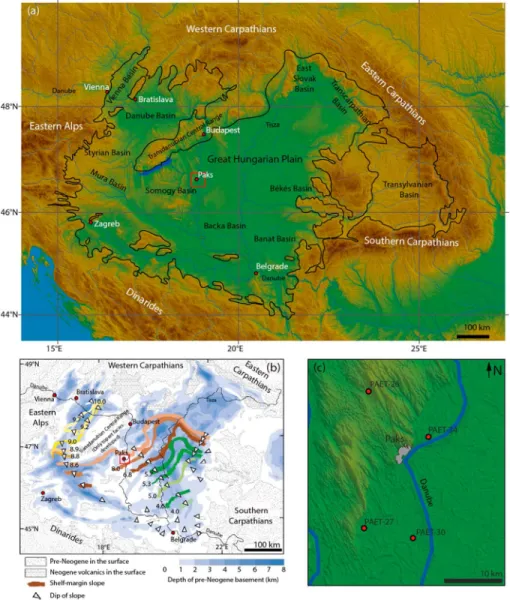
Figure 1.Overview of the Pannonian Basin and location of the study area. (a) Digital elevation model of the Pannonian Basin (after Horváth et al., 2015). The well cores presented in this study were drilled in the area around the city of Paks, (which is) outlined by the red square on the map. Overlain in black is the approximate outline of the Neogene Pannonian Basin, including all the subbasins (modified from Dolton, 2006). (b) Progradation of the paleo-Danube shelf margin in the Pannonian Basin (in Ma) and depth of the pre-Neogene basement (Magyar et al., 2013). The study area is located on a basement high, with the Pannonian sediments between 500 and 1,000 m in thickness. The shelf margin slope passed the study area somewhere between 8.6 and 8.0 Ma. (c) Zoom-in of the study area and core locations.
Greigite can form in sediments in anoxic marine, brackish or freshwater environments, and even during soil formation (Fassbinder & Stanjek, 1994). It grows authigenically if there is an abundance of reactive iron available to react with sulfide. Under reducing conditions, the iron can detach from silicates, the sulfide source is usually pore water sulfate; the sulfate reduction is a biologically induced enzymatic reaction.
When abundant sulfide is available, greigite will react further to form pyrite. However, if the available sulfide is exhausted by the reactive iron, the reaction process can be arrested at the greigite stage.
Formation and preservation of greigite is thus dependent on sulfide production, organic carbon supply, and the concentration of reactive iron (Roberts et al., 2011). The formation of greigite is commonly linked to diagenetic processes, which can occur over extended time intervals, including formation that significantly postdates sediment deposition (Jiang et al., 2001; Larrasoaña et al., 2007; Musgrave & Kars, 2016; Roberts et al., 2011; Rowan & Roberts, 2006; Sagnotti et al., 2005). Because of this ill-defined acquisition timing, greigite has long been considered an unreliable carrier of the natural remanent magnetization (NRM), at least for the interpretation of relatively short-lived geomagnetic features. A major pitfall of using greigite-bearing sediments for paleomagnetic studies is that they may contain different magnetic polarities in the same stratigraphic horizon due to late diagenetic overprinting (e.g., Jiang et al., 2001), seriously complicating magnetostratigraphic dating.
Multiple generations of greigite, or a combination of late diagenetic greigite and any assemblage of primary magnetic minerals, carrying antipodal polarities, may occur in lacustrine environments (e.g., Horng et al., 1998). This has been previously documented or can be inferred from available paleomagnetic studies in the Pannonian region (e.g., Babinszki et al., 2007; Magyar et al., 2007; Vasiliev et al., 2010).
Understanding of greigite formation processes has significantly improved, and it is now clear that greigite can also form, under specific circumstances, during earliest burial processes and consequently may carry a near-primary magnetization (Chang et al., 2014; Hüsing et al., 2009; van Baak et al., 2016; Vasiliev et al., 2007, 2008). Thus, it should be considered an important NRM carrier in sediments. Reliable paleomagnetic signals can then be obtained from greigite bearing sediments if proper demagnetization procedures are followed.
Here we present new magnetostratigraphic results of a set of 500–700-m-long predominantly greigite-bearing well cores covering the upper Miocene lacustrine succession of the Pannonian Basin near the town of Paks in central Hungary (Figure 1). By using dedicated laboratory experiments, incorporating both thermal (TH) and alternatingfield (AF) demagnetization in combination with detailed rock magnetic analyses, this study aims to resolve some of the previously reported problems and pitfalls associated with magnetostratigraphic dating of Lake Pannon sediments and greigite, in general. We show that it is possible to derive reliable, near-primary polarities from these samples, which provide a realistic magnetostratigraphic correlation for Lake Pannon sediments.
2. Geological Setting and Sampling Locations
The formation and evolution of the Pannonian Basin initiated during the early Miocene and is generally related to subduction and collisional processes occurring in the exterior of the Carpathian chain (Balázs et al., 2016; Fodor et al., 1999; Horváth et al., 2006; Horváth & Royden, 1981; Figure 1a). The Miocene to Pliocene subsidence processes were coeval with the orogenic uplift of the Carpathians (Balázs et al., 2016;
Horváth & Cloetingh, 1996; Horváth & Tari, 1999), which eventually disconnected the Pannonian Basin from the rest of the Paratethys domain (~11.6 Ma; ter Borgh et al., 2013).
The environment went from restricted marine to brackish lacustrine, and the resulting basin infill comprises one of the thickest Neogene non-marine depositional sequences in Europe (e.g., Magyar et al., 2013), bearing locally up to 6–7 km of upper Miocene, Pliocene, and Pleistocene sediments (e.g., Dolton, 2006; G. Juhász et al., 2007; Sztanó et al., 2013). The basin sedimentology records an initial transgression in the form of thin conglomerates/breccias, followed by deep water (calcareous) marls, turbiditic sandstones, slope shales to stacked deltaic deposits, andfinally alluvial/fluvial deposits.
The basin infill is diachronous, with most of the sediment influx coming from the NW (paleo-Danube delta) and to a lesser extent from the NE (paleo-Tisza delta; Magyar et al., 2013; Vakarcs et al., 1994; Figure 1b).
The paleo-Danube shelf gradually prograded from the NW to the SE and overfilled the basin. Slope
progradation rate depended much on the highly differentiated lakefloor morphology and associated water depth (G. Juhász et al., 2013; Magyar et al., 2013; Sztanó et al., 2013). Based on seismic data (e.g., Magyar et al., 2007, 2013; Rumpler & Horváth, 1988), the Pannonian sequence that is present is mostly continuous. The earliest Pannonian and a part of the top of the sequence is eroded away, but the sequence in between is continuous and therefore suitable for paleomagnetic correlations.
The studiedPAETdrill cores are located near the (Hungarian) city of Paks, on the banks of the Danube river, approximately 100 km south of Budapest in Hungary (Figures 1a and 1c). Structurally, they are located above a subsurface basement sill that separates deep subbasins to the west and to the east. The basement of Lake Pannon sediments, consisting of either lower to middle Miocene sedimentary and volcanic formations or Mesozoic and Paleozoic strata, is typically shallower than 700–800 m in the study area.
Most stratigraphic studies of Lake Pannon deposits in the surroundings of the study area were based on fully cored master drillings and seismics. The Pannonian sequence of the Lajoskomárom-1 borehole, located some 40 km to the NE of the Paks area, was nominated as afacies stratotypeof the Pannonian stage (Jámbor et al., 1985). Another fully cored drilling, Tengelic-2, only 20 km southwest of Paks, was carefully investigated from both lithostratigraphic and biostratigraphic points of view (Halmai et al., 1982; Korpás-Hódi, 1982;
Sütő-Szentai, 1982; Széles, 1982). In both wells, the base of the Pannonian sequence is located at a depth of around 670 m.
The fully cored Kaskantyú-2 drill hole is located 40 km east of Paks; its Pannonian sequence was analyzed for biostratigraphy, magnetostratigraphy, and seismic stratigraphy (Elston et al., 1994; E. Juhász et al., 1996, 1997;
Lantos et al., 1992; Magyar et al., 1999; Pogácsás et al., 1994; Tóth-Makk, 2007). Finally, another set of wells within the Paks area dates back to the 1990s. Of these cores, only the organic-walled microplankton zonation was published (Sütő-Szentai, 2000). Mapping of the shelf margin across the Pannonian Basin by seismic correlation was carried out by Vakarcs et al. (1994) and Magyar et al. (2013).
These studies show that the Pannonian sediments in the Paks area are truncated at the top by a regional unconformity with an age close to the Miocene-Pliocene boundary (Magyar & Sztanó, 2008). In deep depocenters the sequence develops from the middle Miocene (regional Sarmatian stage) with continuous sedimentation. In structurally higher positions, it unconformably overlies older Neogene or pre-Neogene basement formations with a significant hiatus including the oldest strata of the upper Miocene (regional Pannonian stage).
In both cases, the bulk of the Pannonian sequence belongs to the Congeria praerhomboidea and C.
rhomboideasublittoral mollusk biozones, theProsodacnomyalittoral mollusk zone, and theSpiniferites validus andGalecysta etruscadinoflagellate zones, all of late Miocene age. The exact time span of these zones was estimated by cross correlation of mammal biostratigraphic data, radioisotopic age measurements, and magnetostratigraphic analyses across the entire Pannonian Basin (Magyar et al., 1999; Magyar & Geary, 2012). As a result, the age of the Pannonian sequence in the Paks area is estimated to be between 9 and 6 Ma. The shelf margin of the prograding Danube delta was passing the Paks region at 8.2 Ma according to Vakarcs et al. (1994) and 8.0–8.6 Ma according to Magyar et al. (2013; Figure 1b).
Preliminary biostratigraphic studies of the PAET cores indicate that the Pannonian sequences of PAET-26, PAET-27, and PAET-30 belong to the aforementioned biozones, suggesting an age younger than 9 Ma and older than 6 Ma. The lowermost 50–100 m of PAET-34, however, yielded fossils (both mollusks and dinoflagellates) that belong to biozones older than 9 Ma. Therefore, the underlying middle Miocene biozones, if present, are highly condensed.
3. Methods
3.1. Sampling
Samples were collected from four drill cores, PAET-26, PAET-27, PAET-30, and PAET-34 (Figure 1), which are stored in Paks, Hungary. A battery-powered electrical drill was used to obtain standard-sized oriented paleomagnetic cores at an ~1-m resolution. This sampling resolution was not always attainable due to differences in preservation of the cores because of varying lithology. Finer intervals with high clay/mud con- tent were well preserved and were specifically targeted for sample extraction when possible. The upper
~50 m of the cores consist of unconsolidated Quaternary deposits; these were not sampled. Sand-rich
intervals, depending on the sand fraction and coarseness, would completely disintegrate when dry. Plastic cups were used to obtain samples from these intervals; however, these were unsuited for thermal demagne- tization, which is the required demagnetization method for these (greigite-bearing) samples, as will become apparent from this study. A total of 1,438 paleomagnetic cores were collected: 328 from PAET-26 (14.7 to 499.8-m depth below surface, DBS), 280 from PAET-27 (44.4 to 432.1-m DBS), 344 from core PAET-30 (51.5 to 515.8-m DBS), and 486 from PAET-34 (36.7 to 675.6-m DBS). The well cores were rotary drilled, causing the horizontal component (declination) to be nontraceable. Hence, only the vertical component (inclination) is suited for magnetic polarity determination.
Demagnetization behavior was found to be consistent in all four cores, but sample quality and resolution were highest for cores PAET-30 (PJ-XXX sample codes, with XXX denoting the order in which the samples were taken) and PAET-34 (PAP-XXX sample codes). These were used for the magnetostratigraphic correlation.
The occurrence of significant intervals of unconsolidated sands prevented a high sampling resolution in both PAET-26 (PA-XXX sample codes) and PAET-27 (PJ-XXX sample codes). High-quality samples from PAET-26 and PAET-27 could be used for rock magnetic measurements, however, as similar demagnetization behavior was observed in these cores.
3.2. Rock Magnetism
Rock magnetic measurements include determination of the magnetic susceptibility, thermomagnetic runs, acquisition curves of the isothermal remanent magnetization (IRM), and acquisition offirst-order reversal curve (FORC) diagrams. All experiments were performed at the paleomagnetic laboratoryFort Hoofddijk, Faculty of Geosciences, Utrecht University (The Netherlands). The magnetic susceptibility (expressed on a mass-specific basis per sample) of PAET-26 (328 samples), PAET-27 (267), PAET-30 (341), and PAET-34 (349) was measured with a MFK1 susceptometer (AGICO, Brno, Czech Republic) with a 200-A/mfield strength (peak-to-peak) and a frequency of 900 Hz.
Thermomagnetic runs were performed in air with a modified horizontal translation-type Curie balance with a sensitivity of ~5 · 10 9Am2(Mullender et al., 1993); typical signal strength of the 38 measured samples was on the order of 1 · 10 6Am2. The appliedfield was cycled between 100 and 300 mT. Samples of approxi- mately 40 mg were put into a quartz glass sample holder, and the powdered sample was held in place by quartz wool. These samples were subjected to multiple heating and cooling cycles between room tempera- ture and a maximum of 700 °C; heating rate was 6–8 °C/min and cooling rate 10 °C/min.
IRM acquisition was performed on 48 samples on a horizontal 2G Enterprises DC SQUID magnetometer (noise level 2–3 · 10 12Am2) with in-line anhysteretic and isothermal remanent magnetization facilities and an in- house built sample handler (Mullender et al., 2016). Typical strength of the samples was on the order of 1 · 10 5to 1 · 10 6Am2. To minimize the influence of the magnetic starting state, samples werefirst AF demagnetized along three perpendicular directions in afield of 300 mT, with thefinal demagnetization axis parallel to the subsequent IRMfield (Heslop et al., 2004), using an in-house built AF coil. Afterward, they were subjected to 60 peak IRMfields, increasing in a stepwise fashion to 700 mT. The resulting IRM acquisition curves—linear acquisition plot (LAP), gradient acquisition plot (GAP), and standardized acquisition plot (SAP)—are decomposed into coercivity components using the method of Kruiver et al. (2001).
This results in three variables per component; their saturation IRM (SIRM), thefield strength at which half SIRM is achieved (B1/2), and the dispersion parameter (DP), describing the width of the switchingfield distribution.
The cumulative log-Gaussian approach of Kruiver et al. (2001) is limited to IRM coercivity distributions sym- metric in log space. Due to this, in the cumulative log-Gaussian approach, an extra lowfield component is needed tofit a skewed-to-the-left distribution. FORC diagrams allow to detect and assess the domain states and magnetic interaction among particles within a sample. This is presented in terms of both the coercivity and the magnetic interactionfield distribution, that is, theBcandBuaxes, respectively (Roberts et al., 2014).
FORC diagrams were measured using an alternating gradient magnetometer (Princeton Measurements Corporation), MicroMag model 2900 with a 2 T magnet and a noise level of 2 · 10 9Am2and typical signal strength on the order of 1 · 10 7to 1 · 10 5Am2. Sample mass was between 20 and 45 mg, and saturation was achieved with a maximum appliedfield of 1 T, averaging time of 150 ms.
High-resolution FORC diagrams were calculated from 300 FORCs with afield step of 0.766 mT. Processing of the measurements was done with FORCINEL 3.0 (based on Harrison & Feinberg, 2008), which runs on IgorPro.
Smoothing factors (SF) are applied differently in FORCINEL 3.0 compared to most other FORC processing soft- ware (Harrison, Video Manual for FORCinel 3.0, available on wserv4.esc.cam.ac.uk/nanopaleomag/). The square smoothing boxes are defined in theBc-Bucoordinate system instead of the more conventionalBa- Bbcoordinate system. The result is that about half the number of data points are averaged in comparison to the traditional system. As such, a SF of 10 in FORCINEL 3.0 is reasonably similar to a SF of 5 in most other processing software. In this study high-resolution FORC diagrams were obtained for 28 samples representing all lithologies and paleomagnetic component behavior.
Morphologies of the iron sulfide minerals were visualized by scanning electron microscopy (SEM) performed on a JEOL JCM-6000 tabletop-SEM, operated at 10–15 kV. Backscattered electron (BSE) images were made of representative resin-impregnated polished sections. Semiquantitative standard-less chemical analysis was achieved by energy-dispersive X-ray spectroscropy (EDS). EDS spot analysis was performed with a 10-kV beam and measured for the L-line characteristic X-rays for Fe and for the K-line for S. It should be noted that the effective spot volume in EDS spot analysis in relation to the size of the greigite grains, especially when considering thefiner framboids or sheet silicate greigite, can result in background minerals being included in the analysis. This makes identification of the different iron sulfides difficult. Thus, the EDS spectra are a semiquantitative approximation of the Fe:S atomic ratios present in the observed iron sulfides, enabling (probable) identifications of greigite (Fe3S4, At%; Fe = 42.9, S = 57.1) and pyrite (FeS2, At%; Fe = 33.3, S = 66.7).
3.3. Thermal and Alternating Field Demagnetization
NRM demagnetization was accomplished with both thermal (TH) and alternatingfield (AF) demagnetization.
Samples were thermally demagnetized in a magnetically shielded oven (<2 · 10 8T)in a stepwise fashion (12–17 steps depending on the maximum demagnetization temperature) from room temperature typically up to a (variable) maximum of 330–420°C, but up to 580 °C if required.
Small thermal increments (10 °C), which are smaller than generally used in thermal demagnetization, were implemented between temperatures of ~260 and 310 °C (up to 340/350 °C for PAET-34 samples), to distin- guish between different potentially antipodal greigite components. Samples were selected evenly through- out the cores, with an emphasis on thefiner lithologies where possible: 60 samples for PAET-26, 79 samples for PAET-27, 168 for PAET-30, and 191 samples for PAET-34. Typical sample signal was on the order of 1 · 10 9 1 · 10 8Am2, that is, well above the instrumental noise level.
Demagnetization was consideredfinished when the remanence was reduced to<10% of the starting NRM.
After each heating step, the NRM was measured on a 2G Enterprises DC SQUID magnetometer with a noise level of 3 · 10 12Am2. Alternatingfield demagnetization up to 100 mT was performed on batches consisting of 96 samples from cores PAET-26, PAET-27, and PAET-30. This was achieved on a 2G Enterprises DC SQUID magnetometer with attached AF demagnetization coils and an in-house built robotized sample handler (Mullender et al., 2016). This allowed comparison to the TH results. No AF demagnetization was done for core PAET-34 as AF demagnetization was not deemed useful anymore at that stage of the project. We used a pro- tocol to compensate for any possible gyroremanent magnetization (Mullender et al., 2016), which greigite- bearing samples are prone to acquire during AF demagnetization.
Pyrite-rich samples are prone to having their NRM masked by the formation of magnetite at elevated temperatures during thermal demagnetization, which is particularly problematic with the composite NRMs presented here. A batch of 75 evenly spaced samples from PAET-30 was selected, to investigate if this pro- blem can be overcome by a combination of TH and AF demagnetization. Selected samples were evenly spaced throughout the core and selected on high magnetic susceptibility. These samples were thermally demagnetized up to ~300–310 °C and further demagnetized using AF. All demagnetization results were interpreted using the software available on www.paleomagnetism.org (Koymans et al., 2016).
4. Results
4.1. Multipolarity and Single-Polarity Behavior in Thermally Demagnetized Samples
An overview of typical NRM behavior in the cores is shown in Figure 2. Very weak samples resulted in so-calledspaghetti plotZijderveld diagrams (Figure 2a), which are too noisy to be interpreted and were discarded. These are more dominant in the cores consisting of relatively coarse material (PAET-26 and PAET-27) and generally made up around ~10% of the samples. Two other groups of NRM behavior are
distinguished: samples with a single-polarity (S-type) NRM (Figures 2b and 2c) and samples with a complex composite multipolarity (M-type) NRM (Figures 2d–2f), which represent ~25–35% and ~55–65% of total samples respectively. Note that the S-type and M-type terminology introduced here does not refer to magnetic carriers present in the samples but solely to the demagnetization behavior observed.
The S-type samples, of both normal and reversed polarity, have a single stable NRM starting at ~100–180 °C and generally up to ~350–420 °C (Figure 2b), with no visible clustering in the low-temperature (LT, ~100 to 230–250 °C), medium-temperature (MT, ~230–250 to 300–310 °C), and high-temperature (HT, ~300–310 to 350 °C) ranges observable in the M-types (summarized in Table 1). S-type samples occasionally need to be demagnetized up to higher temperatures (~500–580 °C) due to other primary magnetic carriers (e.g., detrital/biogenic magnetite). It should be kept in mind that when this is required, the magnetite contribution to the NRM is only minor.
The M-type samples show two, often three, NRM components. From room temperature to ~100 °C the behavior is typically random. A low- temperature (LT) component (typically based onfive or six demagnetiza- tion steps) is observable in the range from ~100 to 230–250 °C (Figures 2d–2f). An antipodal medium-temperature (MT) component (four to six demagnetization steps) is identified between 230–250 and 300– 310 °C. Above 300–310 °C we identify a high-temperature (HT) component (two tofive demagnetization steps), which is generally stable to approxi- mately 350 °C. In some samples these components are difficult to separate, because one of the components is only observable as a cluster. This is often the MT component (Figure 2f), but also, the LT and/or HT compo- nents can be observed as clusters.
The LT component is often taken as a viscous (Bruhnes) signal. However, all components occur in both polarities; that is, the LT (and HT component) can be either normal or reversed with the MT having the opposite Figure 2.Overview of representative Zijderveld diagrams (Zijderveld, 1967) for thermally (TH) demagnetized samples.
Open (closed) circles represent inclination (declination). The sample code contains the name (PJ for PAET-30), demag- netization method and depth. (a) Very weak sample, resulting in a spaghetti plot. (b, c) S-type samples. (d, e) M-type samples. (f) M-type sample, with a cluster in the MT range, making it hard to distinguish from S-type samples.
Table 1
Summary of the Individual Components Observed in the M-Type Samples and the Temperature Ranges in Which They Occur
Component
Temperature minimum
Temperature maximum
Viscous 20 °C 100–120 °C
Low temperature (LT) 100–120 °C 230–250 °C
Medium temperature (MT) 230–250 °C 300–310 °C
High temperature (HT) 300–310 °C 350 °C (+*)
Note. The HT component temperature maximum can be a lot higher if there is any significant contribution of other primary magnetic minerals with a higher unblocking temperature (e.g., magnetite and hematite). A minimum of four data points is suggested for every component; the necessary T steps can be derived from the temperature range of each component; for example, the HT component is best interpretable when taking T steps of 10 °C.
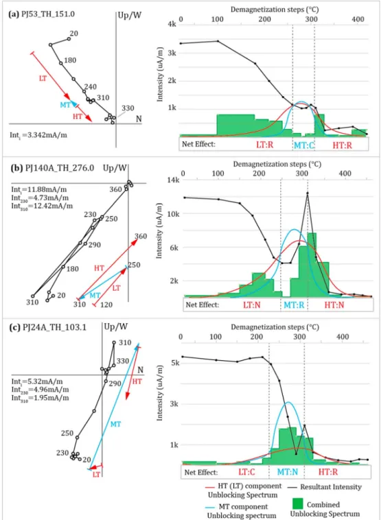
polarity. Furthermore, if they are well resolvable, the LT and HT components in all samples are equal in polar- ity (see supporting information S2). Thus, the LT temperature range in this study does not indicate viscous behavior (also, the upper temperature is too high to be of viscous origin). The LT and HT components may be residing in the same magnetic carrier given the greigite dominance in our samples. This thermal demag- netization behavior is illustrated in the unblocking spectra (strictly speaking, in the case of greigite: chemical alteration spectra) in Figure 3 for three M-type samples with increasing MT:HT ratios. From the thermal demagnetization behavior and combined unblocking spectra we can schematically illustrate the individual components of the M-type samples; the unblocking spectrum due to the MT component becomes more con- fined and steeper when its proportion increases.
As a result, between approximately 230–250 and 300–310 °C the MT component is chemically altered com- paratively more rapidly than the LT/HT components, thus causing thenet polarityto change in this tempera- ture range (if the component carries a significant portion of the NRM). The opposite is true for the LT and HT temperature ranges (at the HT range the MT component is mostly gone).
The S-type and M-type samples can be hard to distinguish in cases where one of either component is predo- minantly present. Thermal demagnetization diagrams of samples with a low MT:HT component ratio show a cluster in the MT range and demagnetize rapidly in the HT range (Figure 3a). This cluster in the MT range (~240–310 °C) hints at a different polarity, which is often not interpretable from the Zijderveld diagram.
Similarly, it is easy to overlook the LT or HT component in diagrams of samples with very high MT:HT ratios (Figure 3c). In these cases, LT can be used as an indicator of HT and vice versa if it is interpretable in the Zijderveld diagram. In this study, the LT components were always interpreted separately in the Zijderveld diagrams.
Samples were divided into two quality groups (Q1 and Q2, respectively), based on maximum angular devia- tion (MAD) values, amount of consecutive data points, whether or not the demagnetization plots show linear trends and their unblocking temperature/coercivity range. The Q1 group for S-types shows a linear decay toward the origin (generally MAD<15°, the majority<10°) and is plotted to a minimum of four consecutive data points. The LT, MT, and HT components of the M-type samples are interpreted and classified indepen- dently. Due to the nature of the M-type samples, the components do not necessarily show a linear decay toward the origin, as net magnetization can increase (e.g., Figure 3b, MT component). The obtained direc- tions of Q1 components of M-type samples do, however, pass through the origin. Due to the small tempera- ture ranges of the MT and HT components and the unpredictable nature of the M-type samples, the conventional standards (Van der Voo, 1990) were at times hard to adhere to; thus, in some cases the MT and HT components were resolved with a minimum of three data points.
Q2 samples fall outside of these criteria and are not used for the polarity zone correlation to the geomagnetic polarity time scale (GPTS). However, they generally agree with the directions of the Q1 samples and often reinforce the interpretation. The inclination values of M-type sample can be substantially lower than the expected values (~60/ 60° for normal/reversed) for this area due to the combined demagnetization of the different components with opposite polarities.
4.2. Rock Magnetic Evidence for Greigite Dominance
We divide our samples into two groups based on their rock magnetic properties, termed Type A and Type B.
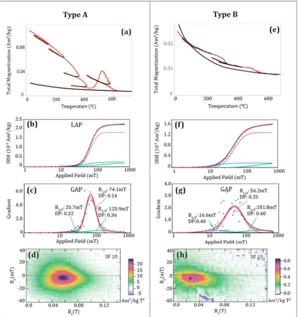
Two extreme examples, with archetypical behavior, are given in Figure 4. Both Types A and B clearly indicate iron sulfides, and most likely greigite, as the dominant magnetic carrier, particularly given their thermomag- netic behavior in air which is typical of greigite. On heating of Type A samples greigite decomposes up to a higher temperature than Type B samples (Figures 4a and 4e). Note that in our study, the Type A rock mag- netic properties appear to be exclusive to demagnetization S types. Type B behavior is always observed in M-type samples and is most obvious when a large part of the NRM is contained in the MT component (high MT:LT + HT ratio). However, Type B rock magnetic properties can also be present in S-type samples. The remaining S-type samples, and M-types with a lower MT/(LT + HT) ratio, have rock magnetic behavior in between the two examples shown.
The terms S-type and M-type denote the single-polarity and multipolarity behaviors observed in Zijderveld diagrams during thermal demagnetization, and not their rock magnetic properties, and thus magnetic car- riers responsible for the paleomagnetic signals of those samples. The reason for this distinction will be
Figure 3.Thermally demagnetized M-type samples with varying MT:HT ratios increasing from sample A to C (left), with their corresponding decay curves and unblocking spectra (right). We present schematic representations of the unblock- ing spectra for the individual and antipodal MT (blue) and LT/HT (red) components derived from the total unblocking spectrum (green columns) and demagnetization behavior. The net effect of these overlapping spectra is indicated below the graphs as component followed by observable behavior. C: (cluster), N: (normal polarity), R: (reversed polarity).
(a) Sample with a low MT:HT ratio. In the Zijderveld diagram, the MT component is identified as a cluster in the 250–300 °C range. Only the combined LT/HT component is clearly interpretable. (b) Sample with a higher MT:HT ratio, which is identified in the Zijderveld diagram as a clearly contrasting (reversed) polarity in the MT range. (c) Sample with a high MT:
HT ratio, resulting in a cluster in the LT range and a small reversed component in the HT range, with a large normal component in the MT range.
discussed later. First, we describe the main magnetic properties; for a more detailed magnetic property description along with an overview of six samples exhibiting varying degrees of Type A and B behavior the reader is referred to the supporting information (A).
Type A: Thermomagnetic runs (Figure 4a) decrease irreversibly in magnetic moment up to 400 °C followed by a (variable) peak in magnetization between 400 and 580 °C. At higher temperatures the magnetic minerals are oxidized to hematite in amounts below the limit of detection of the instrument, that is, indistinguishable from the diamagnetic and paramagnetic matrix minerals that constitute close to 100% of the samples. The decrease up to 400 °C is typical of thermochemical alteration of greigite, which reacts to a paramagnetic iron sulfate between 250 and 350–400 °C (Chang et al., 2008; Dekkers et al., 2000). The increase in magnetism from 400 to 500 °C is caused by thermal alteration of pyrite, forming magnetite as a new magnetic mineral phase. This neoformation of magnetite masks detec- tion of other possibly originally present magnetic minerals. It also may interfere with thermal demagnetization of the NRM. This is observed for both types and is present throughout all cores.
Figure 4.The two types of rock magnetic properties found in most samples. (a, e) Thermomagnetic runs (in air) up to 700 °C. In red/black the heating/cooling cycles.
(b, f) IRM component analyses, linear acquisition plot (LAP), all samplesfitted with three components (shown by the blue, purple, and green curves). (c, g) IRM component analyses, gradient acquisition plot (GAP). (d, h) FORC diagrams. Color scale indicates the FORC density. The smoothing factor (SF) is given for each sample.
The IRM acquisition plots of Type A samples are of good quality (Figure 4b), and the GAP plots (Figure 4c) show a major component (purple curves) with aB1/2value of around 70 mT with a narrow DP between 0.14 and 0.20 (log units). This component contributes ~80% to the total SIRM. TheB1/2and DP values are typical of greigite (e.g., Chang et al., 2014). A high-coercivity mineral (green curves) is likely responsible for the remainder of the signal, which is generally less than 10% of SIRM.
The high-resolution FORC diagrams display concentric contours with a large vertical spread (Figure 4d), which is indicative of single-domain particles with strong magnetostatic interactions (Pike et al., 2001;
Roberts et al., 2014). The FORC contour density maximum atBcof 60 mT is below theBu= 0 axis, behavior associated with greigite. There is no indication for acentral ridge(Egli et al., 2010), so a magnetotactic greigite (or magnetite) contribution, if present, is small in comparison with the diagenetic greigite.
Type B: Thermomagnetic runs are similar to those of Type A samples but are generally noisier and with less pronounced trends (Figure 4e). Nonetheless, pyrite alteration can be observed in the form of a small magnetization increase between 400 and 580 °C (in comparison with paramagnetic hyperbola on thefinal cooling curve), with a broad maximum at ~500 °C. Type B samples show an irreversible decrease in magnetization between ~250 and 300 °C, although it is less pronounced than in typical Type A samples. Importantly, it reacts at lower temperatures than in Type A samples, presumably indicatingfiner greigite particles (Roberts et al., 2006).
IRM acquisition results (Figure 4f) are slightly noisier, and the SIRM are generally an order of magnitude lower than those of Type A samples, despite the fact that the NRM of both types generally possesses equivalent magnetic moments during demagnetization. The IRM acquisition curves (Figure 4g) arefitted with one major component, withB1/2values around 50 mT, and a DP of 0.25–0.30 (log units). This component is interpreted as low-coercivity greigite, as it is on the boundary or just below the acceptedB1/2values for greigite, that is,
~45–95 mT (Roberts et al., 2011). The IRM acquisition could also be interpreted as high-coercivity magnetite or potentially a mixture of magnetite and greigite. However, as unblocking temperatures during thermal demagnetization generally do not exceed ~350 °C, magnetite is unlikely to be present in a significant proportion. Most samples are not saturated above 700 mT, and a highB1/2, high DP component is needed to achieve afit on the IRM curves. This highfield component contributes on average ~10% to the total SIRM. The mean DP is 0.47, andB1/2values range from ~100 to ~360 mT with a mean of ~200 mT. This component most likely represents hematite.
In the FORC diagrams (Figure 4h) the density peak shifts to lower coercivity values of approximately 20–40 mT. The shapes are mostly concentric, with closed contours, or converging on theBuaxes. The vertical density spread is less pronounced for Type B samples but is, like in Type A samples, indicative of fairly strong magnetostatic interactions. A higher SF is needed as the results are noisier than for the Type A samples. The FORC diagrams for Type B samples can be interpreted as a mixture offine-grained greigite and magnetite or as greigite with a smaller grain size distribution.
4.3. Magnetic Susceptibility and Sedimentology
In Figure 5, the magnetic susceptibility is plotted next to the simplified lithological logs. The magnetic sus- ceptibility is variable throughout the cores and is related to the type of sediments. The average of all cores is approximately the same at 10 7m3/kg. The magnetic susceptibility can be a good criterion to select the stronger samples in the cores, as a high magnetic susceptibility correlates well to high magnetic moments (NRM) in these cores. Next to the lithological logs are the formation boundaries. These are based on facies and therefore not correlatable as time lines between the cores. The Endrőd Formation consists of deep lacus- trine calcareous to clay marls. These are followed by siltstone-dominated slope deposits of the Algyő Formation, and superimposed are the stacked silty-to-sandy deltaic deposits of the Újfalu Formation. For PAET-30 and PAET-34 the mollusk biozones are given.
4.4. Scanning Electron Microscopy: Framboidal and Sheet Silicate Greigite
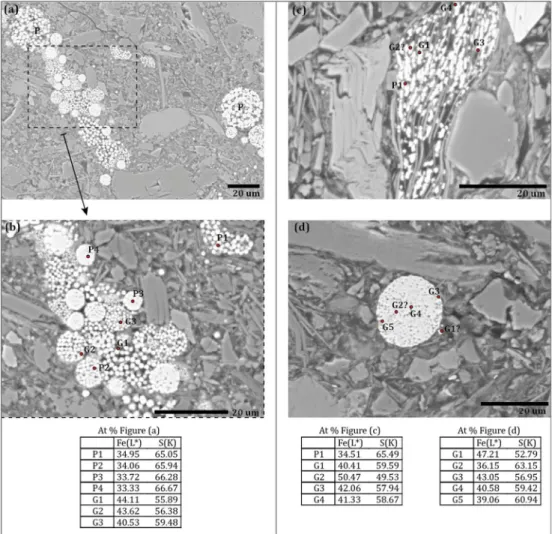
The SEM observations and EDS spectra analyses reveal two distinct suites of greigite present in the Lake Pannon sediments (Figure 6). Type A samples are generally dominated by polyframboidal iron sulfide aggre- gates, in which framboids (both greigite and pyrite based on Fe:S ratios found with EDS analysis) grow in clus- ters (Figures 6a and 6b). Iron sulfide aggregates of both greigite and pyrite grow around and in between the interstitial spaces of the framboids. The largest framboids are generally made up of pyrite.
A second suite of greigite is found in the form of iron sulfides grown within the cleavages of sheet silicates (Figure 6c). EDS analyses show that the sheet silicate iron sulfides are dominantly greigite, although indivi- dual grains of pyrite are also identified. They are generallyfiner grained than the individual grains observed in framboidal structures. Samples that were selected for the SEM observations consisted of both S types (selected based on high magnetic intensity) and M types with a high MT:LT + HT ratio. S types (with Type A rock magnetic properties) appeared to be dominated by the polyframboidal iron sulfide aggregates, with sheet silicate greigite only being present in minor amounts in some samples. M-type samples were always observed to contain an abundance of sheet silicate greigite but likewise always include framboidal greigite, although often less in framboidal aggregates and more in the form of solitary framboids (Figure 6d).
4.5. AF Demagnetization
Figure 7 is a side by side comparison of M-type sister samples demagnetized both thermally and with alter- natingfields. It is immediately evident that the latter cannot distinguish among the LT, MT, and HT compo- nents. The two or three NRM components with opposite polarity observable in TH demagnetized samples are as a rule contained in a single NRM component when using AF demagnetization on the same (sister) samples.
The polarity obtained with the AF method is equal to whichever of the M-type components is the dominant one concerning intensity. In many cases this is the MT component (Figure 7a), although the HT component can be dominant as well (e.g., Figure 7b). For S-type samples, AF and TH demagnetization yielded the same polarity.
4.6. NRM Polarity Patterns
The obtained demagnetization inclinations are plotted in Figures 8 (PAET-30) and 9 (PAET-34). The inclina- tions of the MT and HT components for M-type samples and inclinations for the S-type samples are Figure 5.Magnetic susceptibility (log scale) next to the simplified sedimentary logs of PAET-26, PAET-27, PAET-30, and PAET-34. Magnetic susceptibility in black.
Moving average over 5 points in red and moving average over 15 points in blue. Depth in meters below surface on the vertical axis. Mollusk biozones given for PAET-30 and PAET-34 next to lithological logs.
plotted separately (Figures 8a–8c and Figures 9a–9c). AF data are presented only for PAET-30 (Figure 8e). The large variety in NRM patterns shows the difficulties in obtaining a coherent magnetostratigraphic pattern from these types of sediments. The inclination plots all start at approximately 50-m DBS (depth below surface). In general, the Q2 (open circles) seems to coincide with the high-quality (Q1; closed circles) results. The AF results depict a very erratic polarity pattern (Figure 8e), so these cannot be used for reliable magnetostratigraphic dating.
M-type samples occur throughout all the cores but are less abundant between 320 and 450-m DBS in PAET- 30. As expected, the polarity patterns for the MT and HT components are almost completely opposite. It is implied that the contradicting polarities from the composite M-type samples are formed at different times.
Since the vast majority of the LT components reflect the same polarities as the HT components and are deter- mined to be essentially the same magnetic carrier (section 4.2), they can be used to make a more complete stratigraphic framework (see supporting information B). For PAET-34, the LT and HT components are com- bined and used together to interpret the characteristic remanent magnetization (ChRM; Figure 9b).
Figure 6.Representative SEM BSE (back scattered electron) images of Lake Pannon samples and corresponding EDS spec- tra. EDS analysis is based on L-line measurements for Fe and K-line for S. Ideal atomic ratios are given for pyrite (FeS2, At%;
Fe = 33.3, S = 66.67) and greigite (Fe3S4, At%; Fe = 42.9, S = 57.1). (a) Overview picture of an S-type sample (with Type A rock magnetic properties), showing a polyframboidal iron sulfide aggregate, surrounding/interstitial areasfilled by asecond generation of iron sulfides. Largest framboids are pyrite; interstitial framboids occur as both greigite and pyrite, likewise for the surrounding and interstitialfilling aggregates. (b). Zoom-in of (a), with corresponding EDS spectra below; P indicates pyrite, G greigite. (c, d) Representative BSE images of an M-type sample (with Type B rock magnetic properties), which contains both distinct suites of iron sulfides (mainly greigite grown within the cleavages of sheet silicates; c), and iron sulfide framboidal structures, d).
The S-type and HT components (M-type) are very similar, especially for PAET-30 where the demagnetization results, in general, were more stable than in the other cores (Figures 8b and 8c). It implies that the HT com- ponent was formed around the same time as the signal carried by the S-type samples, which is concluded to be of primary or near primary origin. Similarly, the HT component represents a (near) primary signal. These results are plotted together (Figure 8d) and will be used for the magnetostratigraphic correlation. For PAET-34 there are a few discrepancies between the polarity patterns of the S-type and LT + HT components (Figures 9b and 9c), resulting in a few more outliers in the combined polarity pattern (Figure 9d).
During times of frequent polarity reversals NRMs can be produced that are sometimes consistent (S type) and occasionally inconsistent (M type), depending on the duration of the polarity intervals (Jiang et al., 2001). For example, in the long polarity interval found in the lower part of PAET-30 (~350–450-m DBS) the majority of the samples are determined to be S types (Figures 8b and 8c).
The top and bottom of this interval contain M-type samples, but in the middle (~50 m thick) we solelyfind samples that exhibit S-type demagnetization behavior. This interval contains the highest density of S-type samples found in the core. This seems indicative of a delayed acquisition of remanence represented by the Figure 7.Two sets of sister samples demagnetized both thermally (top) and with alternating fields (bottom). Initial intensity and intensities at specific demagnetization levels are given by Int with a subscript indicating the level. The blue and red arrows indicate direction of the MT and LT/HT components respectively with demagnetization steps in °C. The green arrows indicate the AF-based directions, with demagnetization steps in mT. (a) PJ24A, M-type sample with a domi- nant MT component (normal) and minor HT/LT components (reversed). The corresponding AF result is of normal polarity.
(b) PJ140A, M-type sample with a minor MT component (reversed) and a dominant HT/LT component (normal). The corresponding AF result is of normal polarity.
MT component of the M-type samples. Only the uppermost polarity interval (~50–150-m DBS) is comparable in thickness but shows this behavior less clearly. In the uppermost part of the core, the sample quality and density are less, due to the increasing content of coarser sediments (Figure 5). Also, the topmost interval is thinner than the ~350–450-m DBS interval. M-type samples are dominant throughout the rest of the core (~150–350-m DBS), which is a zone containing many short-lived polarity intervals.
This behavior is not apparent in PAET-34 (Figure 9). Between ~570 and 650 m DBS we exclusivelyfind S-type demagnetization behavior and it is likewise predominantly present from ~445 to 465-m DBS. The apparent time lag in PAET-30 is not found in PAET-34; in fact, the middle ~75 m of the long constant polarity Figure 8.Overview of inclinations and corresponding polarity patterns for well core PAET-30. Black (white) represents nor- mal (reversed) polarity. Depth below surface (DBS) on vertical axis in meters. Closed and connected circles represent data of the Q1 quality group, and open and unconnected circles are Q2 samples. Polarity patterns are based on two or more consecutive data points, a single data point is represented as smaller polarityincursionto indicate a possible polarity change. (a) M-type: MT component. (b) M-type: HT component. The polarity patterns corresponding to the M-type MT and HT components are completely opposite, as expected. (c) S-type samples. S-type samples are dominant in the 350–430-m DBS interval, in which relatively few M-type samples occur. (d) M-type: HT component and S-type samples combined, as they are both interpreted as the ChRM (early diagenetic). (e) Alternatingfield demagnetization results. Note the amount of polarity intervals compared to (d).
interval between ~460 and 600-m DBS is completely dominated by M-type samples. This complicates magnetostratigraphic interpretation. Especially when considering that the MT component can be the dominant component and obscure the HT component, this could potentially lead to inconsistent polarity patterns. Thus, the identification and separation of the MT and HT components are deemed mandatory and short polarity periods must be treated with caution.
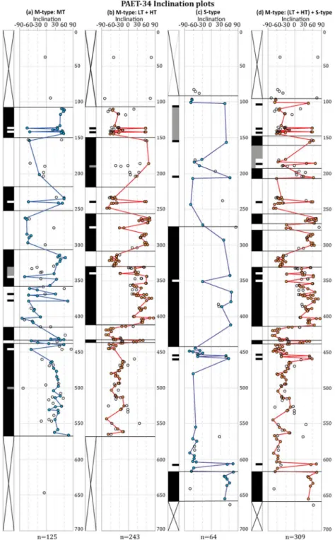
Figure 9.Overview of inclinations and corresponding polarity patterns for well core PAET-34. Black (white) represents normal (reversed) polarity. Gray is used for ambiguous intervals. Depth below surface (DBS) on vertical axis in meters.
Closed and connected circles represent data of the Q1 quality group, and open and unconnected circles are Q2 samples.
(a) M-type: MT component. (b) M-type: LT + HT components. (c) S-type samples. (d) M-type: LT + HT components and S-type samples combined.
5. Discussion
5.1. Mineralogy of MT and HT Components
Based on the rock magnetic properties (Figure 4 and supporting information S1), we found that the predominant magnetic carriers in our samples are magnetic iron sulfides. The magnetic signal found in Type A samples are argued to be caused by an early diagenetic (SD) greigite based on Curie balance measurements, IRM acquisition curves, FORC diagrams, and thermal demagnetization behavior. Samples with Type B rock magnetic properties are also likely dominated by greigite, with a grain size distribution that includesfiner-grained greigite in comparison with the Type A samples. Alternatively, the rock magnetic results for some samples can be indicative of a mixture of greigite and high-coercivity magnetite.
However, as unblocking temperatures during thermal demagnetization of the NRM generally do not exceed
~350 °C, magnetite is unlikely to be present in a significant proportion.
M-type samples always exhibit Type B rock magnetic properties, which is most apparent when a large proportion of the NRM resides in the MT component. Based on the polarity patterns of the individual components of the M-type samples and the S-type samples, we interpreted a delayed acquisition of the NRM residing in the MT component. As the rock magnetic properties indicate a dominance of iron sulfides (greigite), this implies that both the MT and LT + HT components are carried by a form of greigite. The MT component records a delayed acquisition, while the LT and HT components are consistent with the results of S-type samples, and therefore is interpreted as an early diagenetic greigite. Rock magnetic investigations exclude other magnetic carriers as significant contributors to the paleomagnetic signals. Both magnetic carriers responsible for the MT and HT components are interpreted as authigenic greigite. This explains why the components in M-type samples exhibit rock magnetic properties (Type B) that are close to the Type A rock magnetic properties.
The presence of two different greigite components is confirmed by SEM observations and EDS analysis of representative samples (Figure 6). Type A samples are dominated by poly-framboidal aggregates. During early diagenesis at shallow depths and in the presence of abundant reactive iron, a polyframboidal pyrite generation is considered thefirst to grow (Roberts & Weaver, 2005). A second generation of smaller (and occasionally misshapen) iron sulfide framboids and iron sulfide aggregates then grows around and in between thefirst-generation pyrite (observable in Figures 6a and 6b). The polyframboidal aggregates are probably the result of the pyritization of organic matter (Raiswell, 1982) and are very common in greigite- bearing sediments (e.g., Aben et al., 2014; Jiang et al., 2001; Roberts & Weaver, 2005; Rowan & Roberts, 2006; Sagnotti et al., 2005). The greigite either grows contemporaneously or postdates the second generation of pyrite. While this form of authigenic greigite is in essence never of primary origin, it is likely limited to the top few meters of the sediment column (Benning et al., 2000; Berner, 1984) and therefore near primary.
Type B samples contain both greigite framboids/aggregates and authigenic greigite grown within the cleavages of sheet silicates. The near-primary framboids are inferred to be expressed as the LT and HT components in the Zijderveld diagrams. The sheet silicate greigite, while abundantly present due to the plethora of reaction sites within sheet silicates, is very slow to form due to the slow rate at which sheet silicates react with iron sulfides (Roberts & Weaver, 2005). This type of greigite is therefore considered to carry a late diagenetic magnetic signal. The sheet silicate greigite is responsible for the composite NRM behavior so prevalent in Lake Pannon sediments and represents the MT component. Note that the presence of sheet silicate greigite does not mean that M-type demagnetization behavior will be found. During a sufficiently long interval without a reversal of the Earth’s magneticfield (i.e., long chrons) sheet-silicate greigite can record a delayed acquisition of the paleomagnetic signal without an antipodal NRM component, as the polar- ity in which the individual components grow will be the same. These samples would be classified as S types.
The implication is that S types can exhibit both Type A and Type B rock magnetic properties and, therefore, can contain solely early diagenetic greigite in the form of (poly) framboidal greigite or a mixture that includes late diagenetic greigite in the form of sheet silicate greigite. M types exhibit Type B rock magnetic properties, which represent a mixture of early and late diagenetic greigite, as they always contain sheet silicate greigite to a significant extent. In the studied Lake Pannon sediments, deposited during the upper Miocene, most polarity intervals are of relatively short duration. Most S types exhibit Type A rock magnetic properties and are dominated by early diagenetic framboidal greigite; S types are less common than M-type samples, although we did observe sheet silicate greigite occasionally in some S-type samples. Both S types and M
types always contain greigite of an early diagenetic nature (and occasionally minor amounts of other primary magnetic minerals). Therefore, the possibility that S-type samples might have a composite NRM is less relevant for the magnetostratigraphic correlation: if they contain HT interval greigite, their NRM is near primary.
Multiple generations of greigite growth, or late diagenetic greigite growth, are commonly reported in the literature (e.g., Horng et al., 1998; Jiang et al., 2001; Roberts et al., 2005; Roberts & Weaver, 2005; Rowan &
Roberts, 2006; Sagnotti et al., 2005). Horng et al. (1998) also report inconsistent magnetic polarities in the Tsailiao-chi section (SW Taiwan). Polarities from detrital pyrrhotite and magnetite components are consistent with nannofossil biostratigraphy, whereas a delayed formation of greigite is responsible for antiparallel NRM components. Jiang et al. (2001) report multipolarity samples with detrital magnetite as carrier of the primary signal and late diagenetic greigite as carrier of a late, secondary signal. Their results show contradictory composite NRMs similar to the M-type samples reported here. A late diagenetic growth of greigite from siderite was found responsible for remagnetization in a core from the Ross Sea, Antarctica (Sagnotti et al., 2005). These studies exemplify common issues with ChRMs residing in greigite, which in many cases can be solved by careful stratigraphic and rock magnetic analysis.
Summarizing, in the present study early diagenetic greigite, grown as framboids/aggregates, carries a near-primary NRM signal. A late diagenetic component in the form of greigite grown within sheet silicates carries a secondary, often antiparallel, late diagenetic NRM signal. Detrital magnetite is occasionally found to add to the ChRM in samples with a higher unblocking temperature.
5.2. Magnetostratigraphic Correlation
Figure 10 depicts the proposed magnetostratigraphic correlation. The polarity patterns are based on the magnetostratigraphic framework that combines the Q1 samples of the M-type (LT +) HT and S-type data.
Following the dinoflagellate and mollusk biozones, the stratigraphic successions of both cores were correlated between 9 and 6 Ma, except for the lowermost ~100 m of PAET-34, which is likely older than 9 Ma.
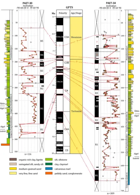
For the PAET-30 core, correlation yields four distinct normal (N1–N4) andfive reversed (R1–R5) intervals, which are used to correlate to the GPTS (Hilgen et al., 2012). We correlate our N1 to Chron C4n.2n (7.695–8.108 Ma), N2 somewhere between 7.285 and 7.695 Ma (most likely to C4n.1n), N3 to C3Br.1n (7.251–7.285 Ma), and N4 to Chron C3Bn (7.140–7.212 Ma). The key to this correlation is the long normal polarity N1 found from ~325 to 440-m DBS. Two normal intervals are expected between 221 and 321-m DBS for this correlation to work. Based on the assumption of continuous sedimentation with a relatively constant rate in this part of the core, a reversal is expected somewhere in our R2 or N2 intervals. The missing reversal is proposed to be found either as a thin reversed polarity interval in the N2 interval or, less likely, as a small normal polarity interval in R2, which would require a marked change in sedimentation rate. A single normal data point hints at a second normal interval in R2. The age of the studied interval of PAET-30 is somewhere between a maximum of 8.77 Ma for the bottom and a minimum age of 6.73 Ma for the top.
Alternative correlations of, for instance, N1 to C4An, or N3-N4 to C3An.1n-C3An.2n are precluded by biostratigraphy, as this would make parts of the succession fall outside the commonly accepted age range of the Pannonian biozones (especially the Congeria rhomboidea sublittoral mollusk biozone in N4 and Prosodacnomya vutskitsilittoral mollusk biozone in N1 are dated between 9 and 6 Ma).
For core PAET-34 we identifiedfive distinct normal (N1–N5) andfive reversed zones (R1–R5), plus some less robust short normal and reversed intervals in the top (Figure 10). We correlate our N1 to Chron C4An (8.771–9.105 Ma), N2 to C4r.1n (8.254–8.300 Ma), N3 to C4n.2n (7.695–8.108 Ma), N4 to C4n.1n (7.528–7.642 Ma), and N5 to Chron C3br.2n (7.454–7.489 Ma). The top of PAET-34 is more difficult to interpret, due to more outliers and some intervals with a lack of data (e.g., ~200–230-m DBS, due to a thick sand interval).
We tentatively correlate the normal interval above R5 to the normal zones in the top of C3B and the overlying long reversed interval to C3An.1r (Figure 10). In this configuration, the maximum age in PAET-34 is 9.11 Ma, while the minimum age might be ~6.73 Ma. The entire correlation from N1 to N5 is plausible but contains unexpected outliers, while such samples are absent in PAET-30. This difference might be due to some erroneous top of the core arrows on the core segments in the depository and/or sample extraction/measurement mistakes or misinterpretation of samples where late diagenetic remanence is
dominant and the MT component in a M-type sample is mistaken for an S-type sample. However, careful thermal demagnetization should give an indication of this due to the different unblocking temperatures of the early and late diagenetic greigite.
The change of sedimentation rates through time can be inferred from the age-depth graphs in Figure 11. The proposed magnetostratigraphic correlations correspond to average sedimentation rates of approximately 29 and 27 cm/kyr for PAET-30 and PAET-34, respectively. The rates are very similar in both cores and represent sedimentation rates that are plausible for a lacustrine to deltaic depositional environment (de Leeuw et al., 2013; Jorissen et al., 2018). In both well cores an upward change from finer slope deposits (Algyő Formation) to coarser deltaic deposits (Újfalu Formation) is observed, so an increase in mean sedimentation rate is expected toward the top of the successions (Figure 3), which is observed for PAET-30, but not for PAET-34.
Figure 10.Magnetostratigraphic correlation for PAET-30 and PAET-34. GPTS from Hilgen et al. (2012). Black (white) represents normal (reversed) polarity. Gray is used for ambiguous intervals. Depth below surface (DBS) on vertical axis in meters. Closed and connected circles represent data of the Q1 quality group, and open and unconnected circles are Q2 samples. Correlations are based on the M-type: HT and S-type samples. Lithological logs and formation boundaries are given next to each magnetostratigraphic correlation.
For PAET-30, the deltaic sequence is interpreted to start at ~375-m DBS. The sediments remain relativelyfine grained, with major sand bodies appearing above 200 m, which is coeval with slightly increasing sedimentation rates in the intervals N3, R4, and N4. In PAET-34 the sedimentation rate increases slightly above ~330 m, with the sandier intervals in the core starting at ~260-m DBS. On a larger scale, however, no clear correlation of the sedimentation rate with the lithology is observed.
The magnetostratigraphic correlations of both studied wells compare well with each other when the stratigraphic information and depths of the cores in the basin are taken into account. As the cores were drilled on basement highs, a part of the older formations that makes up the Lake Pannon sediments is either missing or very condensed. In PAET-30 only the top of the deep lacustrine marls (Endrődi Formation) are present, whereas PAET-34 covers more of these basinal strata. This agrees with the presented age framework where the base of PAET-34 is older than the base of PAET-30. Although the age correlations for the top of the cores are less precise, they both seem to have a similar age for the top (~6.75 Ma), corresponding to a similar stratigraphic depth (70–100-m DBS).
The progradation of the paleo-Danube shelf margin in the study area, based on seismic correlation of clinoforms (from shelf break to toe of slope), most likely occurred between 8.6 and 8.0 Ma (Figure 1b;
Magyar et al., 2013; Vakarcs et al., 1994). Slope deposits (Algyő Formation) are found starting around approximately 460 and 560-m DBS for PAET-30 and PAET-34, respectively, corresponding in our correlation to ages of ~8.3 and 8.6 Ma (Figure 10). The stacked deltaic deposits on the shelf itself (Újfalu Formation) Figure 11.Age-depth plot with inferred sedimentation rates in cm/kyr, based on the magnetostratigraphic correlations in Figure 10. GPTS from Hilgen et al. (2012). Compaction was not integrated in the graphs. PAET-30 sedimentation rates in red, PAET-34 rates in black.
start around ~375 and ~400-m DBS for PAET-30 (~7.8 Ma) and PAET-34 (~8.0 Ma), respectively. This shows that our new magnetostratigraphic correlation coincides well with previous sedimentological and seismic data of Lake Pannon, in particular with the reconstruction by Magyar et al. (2013; Figure 1b). The new magnetostratigraphic data can therefore be used to date the boundaries of the biozones for this part of Lake Pannon.
5.3. AF Demagnetization in Lake Pannon Sediments
It was shown that using AF demagnetization on M-type samples results in a single-polarity component, which is equal to the polarity of the dominant thermally derived NRM component (Figure 7). The plotted AF polarity pattern for PAET-30 (Figure 8e) shows significantly more polarity reversals than when one plots the HT component and S types (Figure 8d) and confirms the unreliability of AF demagnetization in the studied sediments. A polarity pattern based on AF data would contain an erroneous amount of polarity reversals, especially in intervals where M-type samples dominate (e.g., in the 200–300-m DBS interval for PAET-30, Figure 8e). Only intervals dominated by S-type samples will result in a consistent and correct polarity pattern (e.g., 320 to 450-m DBS). As neither the MT:HT ratio in M-type samples nor the occurrence of M-type versus S-type samples can be predicted, AF data should not be considered for magnetostratigraphy of Lake Pannon sediments. In general, magnetostratigraphic dating of greigite bearing sediments should never be done by AF demagnetization alone.
Previous attempts at magnetostratigraphic dating of late Miocene-Pliocene Lake Pannon deposits on the Hungarian territory were largely based on AF demagnetization data (e.g., Lantos & Elston, 1995; Magyar et al., 1999, 2007). Consequently, these studies show polarity patterns that are inconsistent in parts, with an overabundance of polarity zones that are geologically meaningless. In line with the results of this study, Figure 12.Zijderveld projections of three samples that were demagnetized using a combination of TH (top) and AF demagnetization (bottom). The LT (red arrows) and MT component (blue arrows) are demagnetized thermally up until the (second) directional (polarity) change ~300–310 °C (red circles). The same samples are then further AF demagnetized (red arrows) as indicated in the bottom row.