THE IMPACT OF PERCEIVED CORPORATE ENVIRONMENTAL PERFORMANCE ON THE BEHAVIOR OF CAPITAL MARKET
DECISION MAKERS: ANALYSIS OF FOOD INDUSTRY COMPANIES
DEAK,ZS.1*–HUFNAGEL,L.2–HAJDU,I.-NÉ1
1 Department of Food Economy
2 Department of Mathematics and Informatics Corvinus University of Budapest 1118 Budapest, Villányi út 29-43., Hungary (phone: +36-1-482-6200; fax: +36-1-209-0961)
*Corresponding author
e-mail: zsuzsanna.deak@uni-corvinus.hu
(Received 2nd May 2012; accepted 4th October 2012)
Abstract. Environmental protectionism and sustainable development has been gaining increased attention among governments, investors and consumers alike. As a result, firms are facing growing pressure from the various stakeholders to improve their environmental performance. This study is focusing on the food industry, which in recent years has been a subject of increased scrutiny due to their role in resource consumption, waste generation and unsustainable production practices. Our research is aiming to examine how the financial community evaluates the environmental stewardship of food industry companies as proxied by market reactions in response to environmental news. Are all company related environmental news items evaluated equally, and which financial and non-financial firm-specific attributes can influence market responses? Have there been changes in reactions on the stock exchange in the past two decades?
Keywords: environmental performance, food industry, news impact, stock markets, firm-level variables
Introduction
In the nineteenth century the basic focus was on the most efficient and fastest utilization of our natural resources in order to increase profitability. By the twentieth century, however, it became clear that the current rate of utilization will result in unsustainable social and economic development. As a result, the role of socially responsible management and their effects on profitability has become the topic of discussion. The central concern under discussion is how an individual firm's environmental performance influences its financial performance. Does a firm that endeavors to improve its environmental performance gain advantages over its competitors, or does better environmental performance only represent extra costs?
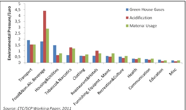
According to a recent study commissioned by the European Commission, the biggest contributors to environmental pressures are food production and consumption, transportation and housing (Fig. 1).
Figure 1. Environmental Pressures per Euro of Spending of Household Consumption Categories
Specifically, the food and drink sector contributes to some 23% of global resource use, 18% of greenhouse gas emissions and 31% of acidifying emissions (ETC/SCP, 2009). The numbers include all resource use and pollution emitted during the production of food from the farm to the supermarket shelf, including the production and application of fertilizers, fuels in agricultural machinery, electricity consumed in food processing plants etc. The United Nation reports similar figures. Of global emissions in 2005, agriculture accounted for an estimated 10-12% of carbon-dioxide, 60% of nitrous oxide and about 50% of methane (excluding emissions from electricity and fuel use).
Globally, agricultural CH4 and N2O emissions have increased by nearly 17% from 1990 to 2005 (IPPC, 2007).
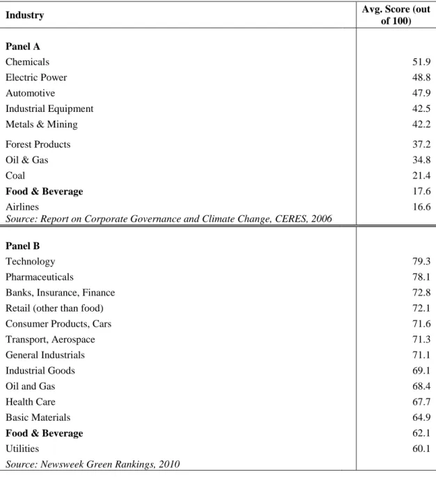
In recent international surveys reviewed, perhaps unexpectedly, some of the traditionally polluting industries fared better than food companies (Table 1).
Table 1. Recent Environmental Performance Rankings by Industry Issued by Media Outlets
Industry Avg. Score (out
of 100)
Panel A
Chemicals 51.9
Electric Power 48.8
Automotive 47.9
Industrial Equipment 42.5
Metals & Mining 42.2
Forest Products 37.2
Oil & Gas 34.8
Coal 21.4
Food & Beverage 17.6
Airlines 16.6
Source: Report on Corporate Governance and Climate Change, CERES, 2006
Panel B
Technology 79.3
Pharmaceuticals 78.1
Banks, Insurance, Finance 72.8
Retail (other than food) 72.1
Consumer Products, Cars 71.6
Transport, Aerospace 71.3
General Industrials 71.1
Industrial Goods 69.1
Oil and Gas 68.4
Health Care 67.7
Basic Materials 64.9
Food & Beverage 62.1
Utilities 60.1
Source: Newsweek Green Rankings, 2010
Based on stakeholder theory, expectation would be that the various concerned parties force companies to improve their environmental performance. If information based regulations works, we should see the effect of environmental news, positive or negative, in the firm’s security prices.
Review of literature
Results obtained in earlier research seeking to uncover the link between firm level social responsibility – of which environmental behavior is a subset – and financial performance have been mixed. Even though, in general, it has been found that companies experience a drop in market value following adverse environmental news, while they experience the opposite effect following good news, the findings are by no means homogenous.
Researchers have utilized various methods to investigate the relationship between environmental and financial performance. They sometimes explored the effects of specific positive (ISO certification) or negative (oil spill) events or actions on firms’
financial variables (company stock prices or balance sheet items such as return on equity – ROE, return on assets – ROA or Tobin’s q). Often they compared portfolios of polluting companies with more environmentally conscious ones (this is basically the same method that socially responsible investment (SRI) fund managers have adopted).
Dowell, Hart and Yeung (2000) in their study categorized US companies based on whether or not they operate at US environmental standards worldwide or adopt lower standards outside of the US where this is permitted. They found a positive correlation between Tobin’s q (the ratio of the stock market value of the company to the cost of its tangible assets) and firm environmental performance. In a later study Konar and Cohen (2001), found that firms that are emitting fewer toxic chemicals, or are threatened with fewer environmental lawsuits, are also likely to have a higher Tobin’s q. In a 2002 paper, King and Lenox posit that it is actually pollution prevention and not pollution remediation that results in better return on assets (ROA). Hamilton (1995) and Konar and Cohen (1997) investigated the effect of the release of the Toxics Release Inventory (TRI) data on the market value of firms, while Lanoie and Laplante (1994) and Klassen and McLaughlin (1996) looked at stock market reactions of companies to environmental news in the media. Klassen and McLaughlin documented significantly positive market reactions to independent third-party awards for environmental performance. In contrast, Gilley et al. (2000) who examined stock market reactions to environmental process improvements found negative results. Muoghalu et al. (1990) examined the impacts of hazardous waste mismanagement lawsuits on capital markets and found that the firms suffer significant losses. These varying results suggest that perhaps the market does not value all types of environmental accomplishments or misconducts equally. Additionally, King and Baerwald (1998) argue that unique firm characteristics influence how events are reported and interpreted when comparing environmental performance. Recent studies (Cormier and Magnan, 2007; Wagner, 2010; Horváthová, 2010) also confirm that these diverging outcomes received could be because of specific firm-level characteristics (such as size, R&D expenditure, advertising intensity, riskiness, leverage, industry, country etc.). This would support the resource-based view of strategic management (see Barney, 1986; Wernerfelt, 1984) based on which a firm’s superior ability to manage their environmental problems and reputation compared to others in the industry could lead to higher returns.
There are fewer articles dedicated to the research of how market reactions developed over time. Dasgupta et al (2005) concludes that the average market reaction to negative events is indeed changing over time. They have examined the period between 1992 and 2000. Blancard and Laguna (2009), when looking at the effects of chemical disasters between 1995 and 2005, however found no significant differences among their selected periods.
Besides the various measurements used to evaluate environmental performance and the question of the specific setting in which the firms operate an additional area of contention is an econometric one. Researchers have observed that stock markets have a certain way of operating. For example, Jegadeesh and Titman (1993) observed that stocks that perform well/poorly over a three- to twelve-month period tend to continue their tendency in the next three to twelve months. This tendency, called the momentum, is an anomaly and has largely been attributed to the cognitive bias of „irrational
investors” who under/overreact to the release of firm-specific information. Furthermore, they have noticed that the error terms do not follow a normal distribution with constant variance. To mitigate these effects researchers have proposed various econometric models (see more in detail in the Methodology section).
The four research questions we seek answers to are therefore the following: how are results influenced
Q1: by the econometric model used,
Q2: by the type of environmental events reported,
Q3: by company level characteristics (both financial and non-financial), and Q4: by the time elapsed?
Methodology
The event study methodology developed by Fama, Fisher, Jensen, and Roll (1969) has become the standard method of measuring stock price reaction to some announcement or event in the financial economics literature. Event studies have been used to test the null hypothesis that markets efficiently incorporate new information and that under the maintained hypothesis of market efficiency, to examine the impact of an event on the wealth of a firm’s shareholders (Binder, 1998).
An event study starts with identification of the event of interest and the event window, which is the time period over which the stock prices of firms will be examined.
Assessment of an event’s impact requires a measure of abnormal return. The abnormal return is the difference between the ex post return and the normal return of a firm’s stock over the event window. Consistent with most event studies, here the “market model" is used to estimate abnormal returns. This model assumes a linear relationship between the return on a stock and the market return (in our case the Standard and Poor’s 500 (S&P500) is used as a proxy for the market portfolio) over a given time period as:
(Eq.1)
where Rmt is the return of the market portfolio for the period t, εit is the zero mean disturbance term, and αi and βi are the parameters to be estimated. In the standard event study framework abnormal returns for firm i on day t ( ) are modeled as prediction errors from the market model:
(Eq.2)
where and are the firm’s estimated parameters over the estimation period. See MacKinlay (1997) and Binder (1998) for a detailed review of event study methodologies.
One can simply estimate the above equation with ordinary least squares (OLS).
However, OLS estimation is based on several assumptions. The first assumption is that the error term εit is serially uncorrelated. However, Lo and MacKinlay (1988) showed that successive returns on individual stocks are indeed correlated; where large returns tend to be followed by further large returns. The second assumption is that the error
term follows a normal distribution with constant variance, that is, it is homoskedastic.
Giaccoto and Ali (1982) documented that if the assumption of homoskedasticity is not met, the parameter estimates are inefficient and thus any inferences based upon them are potentially misleading. Therefore, to measure the effect of a specific event on stock prices one must account for time-varying variance (heteroskedasticity). Engle (1982) developed a model, in which current conditional variance depends on the past values of squared random disturbances called autoregressive conditional heteroskedasticity (ARCH). The ARCH model is modified by Bollerslev (1986, 1987) to allow current conditional variance to depend on past conditional variances as well as the past squared random disturbances. The advantage of the generalized autoregressive conditional heteroskedasticity (GARCH) model is that not only does it model the mean of the returns (Rit), but at the same time allows for time-varying volatility. Since then GARCH models have been widely used in the literature and are found to be suitable in explaining stock price distributions (Bollerslev, 1987; Bollerslev, Engle and Wooldridge, 1988;
French, Schwert and Stambaugh, 1987; Baillie and DeGennaro, 1990).
It has been found (see de Jong et al., 1991; Corhay and Tourani, 1996; Hansen and Lunde, 2001) that the modest gains obtained do not justify the use of more complicated GARCH models and GARCH (1, 1) provides a parsimonious but adequate model specification. The market model corrected for GARCH is:
(Eq.3a)
With variance equation of:
(Eq.3b)
(Eq.3c)
where εit is the error term with mean zero and variance hit. Rit represents daily stock return of firm i on day t and Rmt represents daily return of the S&P 500. Returns are computed as , where Pt is either the stock price for a company on day t or the S&P 500 index.
For our empirical analysis we calculate abnormal returns both with OLS and GARCH specifications. Since we are not only interested in the average abnormal return per event type but also the median return we utilize the standard event study method.
We consider a three day event window with one day added before and after the event day to capture the full effect. From the abnormal returns thus received we calculate a three day cumulated average return (CAR):
(Eq.4)
Thereafter, we want to test if the groups we have created (as described below) are significantly different from each other that is whether the various company characteristics or the passing of time influences the median CAR.
Sample and data description
For our study stock prices of food industry companies that were traded on the New York Stock Exchange (NYSE) and NASDAQ between the periods of January 1990 and December 2010 were collected. Only companies that were continuously traded and have sales greater than $1 million are included in the sample. With a list of keywords and phrases generally used in the environmental news, a search string is created in the Wall Street Journal Factiva database and all announcements that meet the search criteria are downloaded. In the case of news that appeared in more than one publication or multiple times in the same publication, only the news with the earliest publication date is retained. Additionally, days with multiple announcements or days where event windows overlapped are excluded, as in these cases it would be impossible to determine which environmental announcement is responsible for any market reaction. Only days with no additional confounding events, such as dividend and earnings announcements are used.
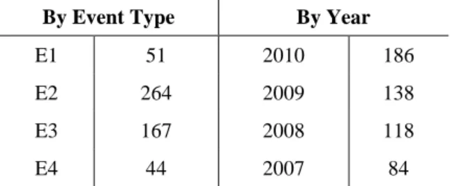
For our research questions we needed to create two sets of data sets. For the development of abnormal returns over time we have used the entire dataset of twenty years. This includes 880 environmental events. For the firm-level variables, due to the availability and volatility of data, only a subset of the last four years was used.
Therefore, for the cross-sectional analysis we are left with 526 environmental events.
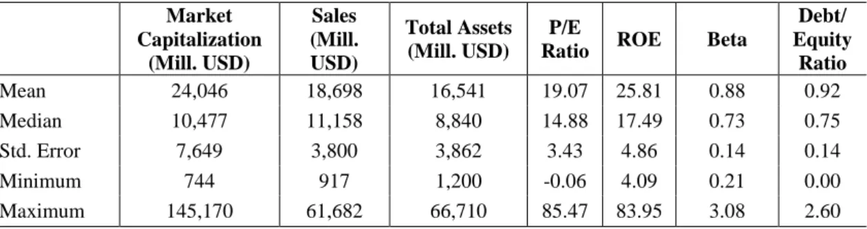
Our sample includes 23 unique firms from 17 primary Standard Industrial Classification (SIC) codes. The study excludes all alcoholic and tobacco related products as they would skew the results due to reputational preconceptions. Table 2 provides descriptive statistics of the sample.
Table 2. Descriptive Statistics of the 23 Sample Firms for Selected Firm-level Financial Variables: Size (assets), Profitability (Return on Equity, ROE and Price Earnings Ratio, P/E), Riskiness (beta), and Leverage (Long-term Debt to Equity Ratio, LEV)
Market Capitalization
(Mill. USD)
Sales (Mill.
USD)
Total Assets (Mill. USD)
P/E
Ratio ROE Beta
Debt/
Equity Ratio
Mean 24,046 18,698 16,541 19.07 25.81 0.88 0.92
Median 10,477 11,158 8,840 14.88 17.49 0.73 0.75
Std. Error 7,649 3,800 3,862 3.43 4.86 0.14 0.14
Minimum 744 917 1,200 -0.06 4.09 0.21 0.00
Maximum 145,170 61,682 66,710 85.47 83.95 3.08 2.60
The food production industry is highly concentrated with the top four players (Nestlé, Unilever, Kraft and Danone) constituting more than 50% of the global market capitalization of the top thirty food companies (Eurosif, 2010). In our study, the average size of companies in terms of market capitalization is over $24 billion, while the mean profitability expressed in the P/E ratio is around 19, which is in line with the industry average.
Given that the environmental news collected consist of different types of events, both positive and negative, it is possible that market reaction varies across different event categories. For example, markets may react to negative news by a larger amount than they do to positive news. By aggregating news items of different types without knowing the sign of the news, could cancel out market reactions and result in an average reaction that is not statistically different from zero. To distinguish the effect of specific events,
the news sample is first divided into positive and negative events and then to external and internal events to form the following four subcategories:
Event type 1: News relating to penalties, government action, lawsuits etc. against the companies
Key words: accident, clean, cleanup, "Department of Justice," "Environmental Protection Agency," fine, lawsuit, notice, order, penalty, settle, spill, superfund, tort, toxic, violation.
Event type 2: Actions taken by the companies to improve environmental performance or perception
Key words: carbon, certification, climate, conservation, donation, eco, EMS, endow, energy, environment, footprint, green, "ISO 14001," LEED, nature, recycling, renewable, reusable, "SA 8000," stewardship, support, sustainability.
Event type 3: Awards, rankings issued by an outside source about the company Key words: admire, award, celebrate, certificate, honor, index, prize, rank, recognition, scorecard, tribute, win, won.
Event type 4: Boycotts, external company reports and studies, other external non- classifiable
Key words: accuse, action, activists, analysis, boycott, contamination, disaster, dump, emission, environment, Greenpeace, incident, rally, report, research, pollution, study.
Event types 1 and 2 focus on events that are direct results of specific internal actions of the companies while event types 3 and 4 are opinions of external parties. Further, event types 2 and 3 represent positive news items while event types 1 and 4 represent negative news (Table 3).
Table 3. Breakdown of Events by Event Types: E1(negative internal), E2(positive internal), E3(positive external) and E4(negative external) and by Years for Cross-sectional Analysis
By Event Type By Year
E1 51 2010 186
E2 264 2009 138
E3 167 2008 118
E4 44 2007 84
The financial variables we consider include size (assets), profitability (return on equity, ROE and Price Earnings Ratio, P/E), riskiness (beta), and leverage (long-term debt to equity, LEV). Non-financial variables include media coverage and green reputation. For company media coverage, we looked at the number of articles related to environmental issues published in the printed media. For environmental reputation we computed an average environmental score based on rankings publish in the media (Newsweek, CRO Magazine etc.), investment fund analyst companies (Maplecroft, KLD) and by NGOs (CERES, CDP). We broke down the companies into two groups
for each of the financial and non-financial variables as shown in Table 4. Accordingly, group 1 of each variable consists of companies with the highest value and group 2 consists of companies with the lowest value of that variable.
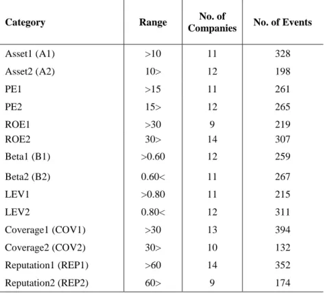
Table 4. Breakdown of the Selected Financial and Non-Financial Firm-level Category Ranges and the Number of Events and Companies in Each Group between the Years of 2007-10
Category Range No. of
Companies No. of Events
Asset1 (A1) >10 11 328
Asset2 (A2) 10> 12 198
PE1 >15 11 261
PE2 15> 12 265
ROE1 >30 9 219
ROE2 30> 14 307
Beta1 (B1) >0.60 12 259
Beta2 (B2) 0.60< 11 267
LEV1 >0.80 11 215
LEV2 0.80< 12 311
Coverage1 (COV1) >30 13 394
Coverage2 (COV2) 30> 10 132
Reputation1 (REP1) >60 14 352
Reputation2 (REP2) 60> 9 174
With the two different econometrics models, we have thus created a total of 14 scenarios to investigate.
For the longitudinal analysis we have created a graphical representation of the development of the CARs for each event type for the twenty-year span examined to visualize the various trends and thus create suitable time periods to be compared.
Results and discussion Cross-sectional analysis
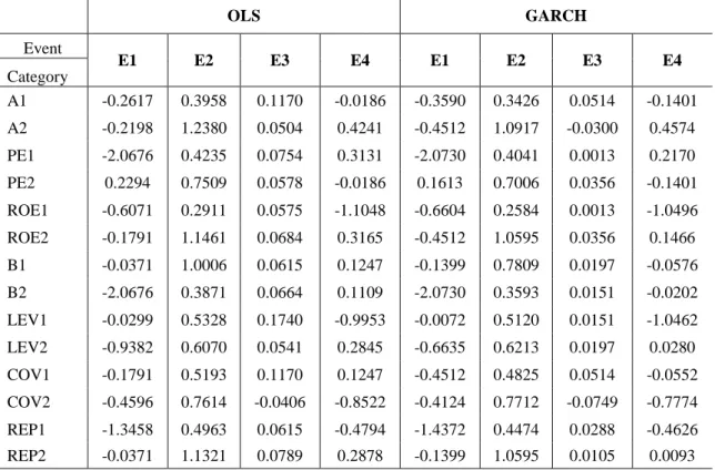
The purpose of our testing was to determine how the event types and various company characteristics influence abnormal returns. Therefore, we wanted to perform a pair wise comparison of the medians for each possible combination. The medians for each group can be seen in Table 5.
Table 5. Median CARs gained per Grouped Firm-Level Variables and Event Types from OLS and GARCH testing
OLS GARCH
Event
E1 E2 E3 E4 E1 E2 E3 E4
Category
A1 -0.2617 0.3958 0.1170 -0.0186 -0.3590 0.3426 0.0514 -0.1401 A2 -0.2198 1.2380 0.0504 0.4241 -0.4512 1.0917 -0.0300 0.4574 PE1 -2.0676 0.4235 0.0754 0.3131 -2.0730 0.4041 0.0013 0.2170 PE2 0.2294 0.7509 0.0578 -0.0186 0.1613 0.7006 0.0356 -0.1401 ROE1 -0.6071 0.2911 0.0575 -1.1048 -0.6604 0.2584 0.0013 -1.0496 ROE2 -0.1791 1.1461 0.0684 0.3165 -0.4512 1.0595 0.0356 0.1466 B1 -0.0371 1.0006 0.0615 0.1247 -0.1399 0.7809 0.0197 -0.0576 B2 -2.0676 0.3871 0.0664 0.1109 -2.0730 0.3593 0.0151 -0.0202 LEV1 -0.0299 0.5328 0.1740 -0.9953 -0.0072 0.5120 0.0151 -1.0462 LEV2 -0.9382 0.6070 0.0541 0.2845 -0.6635 0.6213 0.0197 0.0280 COV1 -0.1791 0.5193 0.1170 0.1247 -0.4512 0.4825 0.0514 -0.0552 COV2 -0.4596 0.7614 -0.0406 -0.8522 -0.4124 0.7712 -0.0749 -0.7774 REP1 -1.3458 0.4963 0.0615 -0.4794 -1.4372 0.4474 0.0288 -0.4626 REP2 -0.0371 1.1321 0.0789 0.2878 -0.1399 1.0595 0.0105 0.0093
Between the two econometric approaches used, negative events have become more negative and positive ones less positive. In fact, some lower positive results have even switched signs. However, the choice of statistical approach did not change the results drastically.
In the first step, we had to test whether the groups thus created have any significant effect on the results. Based on the Kruskal-Wallis test performed the grouping was relevant for both the OLS and GARCH type testing (p<0.05) (Table 6).
Table 6. Results of the Kruskal-Wallis Test for the Seven Firm-Level Categories for OLS and GARCH
OLS GARCH
1,1
Asset 2.246E-05 2.874E-05
PE 1.206E-05 1.631E-05
ROE 5.251E-05 7.074E-05 Beta 1.878E-05 3.074E-05 Lev 0.0005604 0.0005848
Cover 0.001449 0.00167
Rep 8.846E-05 9.926E-05
Consequently, a post-hoc analysis was performed on the CARs gained from our tests.
Since we are performing a number of pair wise comparisons there is an increased chance of committing a Type I error. Therefore, we have run the analysis in a Bonferroni corrected and uncorrected form (Table 7).
Table 7. Results of the Mann-Whitney post-hoc Test (Bonferroni Corrected/Uncorrected) for GARCH prediction errors in the Seven Groups Created from Firm-level Characteristics for the Four Event Types
ROEROE1E1ROE1E2ROE1E3ROE1E4ROE2E1ROE2E2ROE2E3ROE2E4PEPE1E1PE1E2PE1E3PE1E4PE2E1PE2E2PE2E3PE2E4 ROE1E10.01770.05800.96980.71310.00210.07500.1073PE1E14.25E-060.00010.00500.01796.0E-060.00030.0269 ROE1E20.49530.18460.01380.04100.00050.48720.6539PE1E20.00010.03270.33080.40360.13960.12350.0502 ROE1E3110.04470.16171.16E-040.72150.7506PE1E30.00310.91660.94840.80281.85E-030.74720.4917 ROE1E410.384910.76680.00260.07500.1269PE1E40.1390110.99090.21240.93760.5860 ROE2E111110.00120.15320.2661PE2E10.50201110.13270.99740.5981 ROE2E20.05750.01320.00320.07230.03240.00100.0363PE2E20.000210.0519110.01370.0144 ROE2E3111110.02840.9034PE2E30.008211110.38240.4470 ROE2E411111110PE2E40.751911110.40241 AssetA1E1A1E2A1E3A1E4A2E1A2E2A2E3A2E4BetaB1E1B1E2B1E3B1E4B2E1B2E2B2E3B2E4 A1E10.0044020.04090.62670.81836.84E-050.06710.0804B1E10.051310.80790.96980.07050.30810.86330.6912 A1E20.12330.09370.02240.15700.00200.21060.9278B1E210.01460.03914.3E-050.01540.00020.0228 A1E3110.17480.38125.01E-050.90350.4655B1E310.40990.82390.00552.85E-010.78270.4243 A1E410.626010.98080.00050.24650.2190B1E41110.03060.24560.87920.6031 A2E111110.03640.45550.3705B2E110.00120.15330.85690.0001010.00080.0890 A2E20.00190.05670.00140.014410.00120.2440B2E210.4309110.00280.05970.0917 A2E3111110.03360.6573B2E310.0046110.022210.3534 A2E41111111B2E410.638811111 DebtLEV1E1LEV1E2LEV1E3LEV1E4LEV2E1LEV2E2LEV2E3LEV2E4CoverageCOV1E1COV1E2COV1E3COV1E4COV2E1COV2E2COV2E3COV2E4 LEV1E10.4750.91950.46420.28040.35820.95010.9626COV1E10.00070.04110.27670.81560.00160.09900.4856 LEV1E210.07870.01910.00040.86640.00980.1884COV1E20.01870.00890.04730.18560.62850.04830.1679 LEV1E3110.08750.01265.89E-020.39710.8252COV1E310.24880.62080.42921.92E-020.98750.6639 LEV1E410.534910.74990.02620.28890.3196COV1E41110.63560.03680.69390.9795 LEV2E110.01060.35410.00050.05210.0948COV2E111110.15190.51550.7648 LEV2E21110.73230.01280.00420.1345COV2E20.043710.5388110.03400.1889 LEV2E310.27511110.11820.7031COV2E3111110.95260.5926 LEV2E41111111COV2E41111111 ReputationREP1E1REP1E2REP1E3REP1E4REP2E1REP2E2REP2E3REP2E4 REP1E16.67E-050.00270.36250.27100.00040.01980.0365 REP1E20.00190.00560.01630.11300.07500.24290.2591 REP1E30.07640.15710.1680.57081.52E-030.73030.8339 REP1E410.455310.73460.01570.26760.2998 REP2E111110.05480.58570.5484 REP2E20.011710.04250.439110.07660.1025 REP2E30.5546111110.9785 REP2E41111111
Note: Firm-level Categories: Return on Equity (ROE1, ROE2), Price/Earnings Ratio (PE1, PE2), Asset (A1, A2), Leverage-Debt Equity Ratio (LEV1, LEV2), Riskiness-Beta (B1, B2), Media Coverage (COV1, COV2), and Environmental Reputation (REP1, REP2); Event Types: E1(negative internal), E2(positive internal), E3(positive external) and E4(negative external)
Coverage and indebtedness has the least effect, while ROE, PE, beta and reputation produce about the same amount of significant results. Company size (asset), while also on the low end, seems to be the most persistent influence as even after Bonferroni correction half of the significant results remain. For all other categories this is only between 25-36%.
When looking at events within the individual groups, Type E4 events in most cases seem to be too homogeneous to sufficiently differentiate them from any other category (could possibly be because this group was not adequately specified or had the lowest sample count). Less than 20% of the possible pairings produced results and most of these were in the E2-E4 pairing (clearly due to the very strong significance of the positive internal events). With Bonferroni correction this becomes even more pronounced (with only one interpretable result remaining). Type E2 events on the other hand are the most clearly demarcated (above 55%). Median abnormal returns between E1 and E2 (positive and negative internal events) and between E2 and E3 (the two positive event types) are almost always clearly distinct for all categories (68% and 61%). Even after Bonferroni correction we are left with several significant differences.
In case of the E2-E3 pairing, companies with lower ROE and smaller size (group 2), are producing a difference of over 1% in positive CAR in response to positive internal news when compared to positive external news (within their own or the other group).
However, while smaller asset size influences the difference downward (0.03 %), lower return on equity increases it by 0.08 %.
For the E1-E2 pairing, both lower risk and lower indebtedness influences the amount of penalty incurred for environmental infringements. Within the lower risk group companies that implement positive environmental actions gain 2.43% vs. their piers that incur penalties. In the higher risk group positive actions bring an additional 0.42 % abnormal return. For low debt companies positive actions result in an increase of 1.28
% vs. companies with negative internal news. For the high debt ratio companies this is only 1.18 %. Seems that investors do not appreciate additional capital outlays for already indebted companies. Companies with high profitability expectations are penalized by 2.48 % for environmental transgressions, while their less fortunate piers, with already lower PE, lose 2.77 % vs. firms that implement environmental measures.
In this case the better financial situation shelters companies from the full effect of negative news. The dynamics between companies with good and bad reputation is similar, but even more pronounced. Here firms with better green image are shielded from negative effects, as they lose 0.61% less when bad news breaks versus companies with an already bad reputation. In the company media coverage category, the reaction is somewhat unexpected. Here companies that appear in the media less frequently have to face a more pronounced response by the market (by 0.28 %).
Additionally, it’s worth pointing out that for the E1-E3 pairing we can see similar, but less pronounced correlation. While it is true that companies with higher profitability expectations are facing stiffer penalties for infringements they also lose 0.03% less of their CAR compared to firms in worse financial situation, as these firms benefit more from positive outside opinions.
Especially interesting for our study was to see whether the firm level characteristics by themselves contribute to the development of abnormal returns. Therefore, we have highlighted the comparison of groups of similar event types with differing characteristics in Table 8:
Table 8. Significant Differences in Median CAR Between Similar Event Types Based on Company Characteristics*
Asset PE ROE Beta LEV COV REP
E1 O X O O O O O
E2 X O X X O O O
E3 O O O O O O O
E4 O O O O O O O
* Both for OLS and GARCH Note: x marks p< 0.05 or less
In company profitability, ROE impacts E2 while P/E ratio E1 type events. This difference in reaction to the two profitability ratios is understandable as E1 type events have clear monetary consequences that affect the bottom line directly while E2 type events affect the bottom line through investment outlays. Company perceived riskiness (beta) and company size influences E2 type events. Smaller, less profitable companies are rewarded to a greater extent for internal company initiatives (a difference of 0.84 % and 0.86 % respectively). Company indebtedness (LEV), media coverage and reputation do not seem to influence abnormal returns at all between the two groups. Again, after Bonferroni correction only ROE and Asset results remained significant.
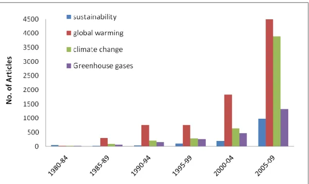
When looking at environmental news in the media, there is a growing trend in the amount of news published in this topic (Fig. 2).
Figure 2. News Articles by Topic in The New York Times between 1980 and 2010
There is also a clear delineation between event types. While the number of negative news items relating to environmental penalties published leveled off over time, reports relating to positive company initiatives were growing exponentially. At the same time,
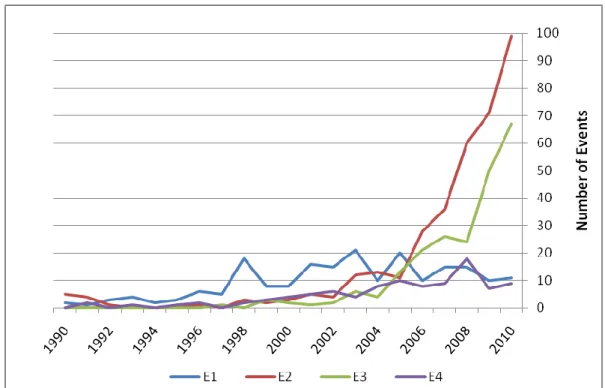
news originating from outside evaluations, both positive and negative, have only appeared regularly in the media after the year 2000. Here, the number of awards and rankings was increasing steadily, while third party negative reports, after an initial spurt, have also stabilized (Fig. 3). This reflects two distinct trends: first the companies have realized the importance of the role of media and are placing greater emphasis on managing their image, and second the non-governmental organizations and investing communities have become increasingly active.
Figure 3. Development of News by Event Types between 1990-2010
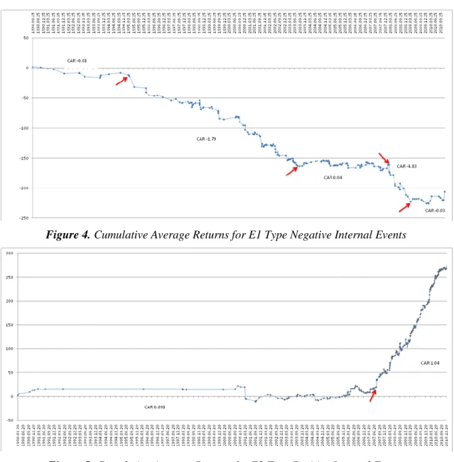
We have examined our four distinct event types and the relating cumulative abnormal returns produced over time. The initial idea of splitting the twenty-year span into equal portions for all events was not feasible as the trends per event type did not overlap and such divisions produced no useable results. Therefore we have looked at each event type separately by creating four portfolios and calculating the cumulative gain/loss over time. For a graphical representation, please see Figures 4-7. Generally speaking the tipping points per event type do not coincide, with some interesting exceptions. In April of 2007, for example, due to a landmark judicial decision in the United States and a crucial IPCC (Intergovernmental Panel on Climate Change) report sentiments toward climate change and the environment improved significantly. As a result, we can see an upward movement in CARs for E2 events and a corresponding dip in CARs for E4 and E1 type events. Shifts in government policy, such as George Bush’s climate plan announcement in February 2003, or Barack Obama’s election in November 2008, were also important events that influenced attitudes of investors.
Figure 4. Cumulative Average Returns for E1 Type Negative Internal Events
Figure 5. Cumulative Average Returns for E2 Type Positive Internal Events
Figure 6. Cumulative Average Returns for E3 Type Positive External Events
Figure 7. Cumulative Average Returns for E4 Type Negative External Events
While all event types show a trend in the generally expected direction, E1 and E2 type events are more homogeneous while E3 and E4 are more cyclical. To verify that our selected periods are well defined we again looked at the pair wise comparison of medians (Table 9).
Table 9. Results of the Mann-Whitney post-hoc Test (Bonferroni Corrected/Uncorrected) for GARCH Prediction Errors for the Selected Time Periods of the Four Event Types
E1 Type Events E4 Type Events
H 21.24 H 9.871
p 0.0002832 p 0.0197
11/2/1994 2/18/2003 2/28/2008 4/6/2009 12/31/2010 8/13/2002 3/21/2007 7/10/2008 12/31/2010
11/2/1994 0.2688 0.9757 0.01572 0.8421 7/20/2004 0.01698 0.9137 0.0520
2/18/2003 1 0.002596 0.02318 0.07465 3/21/2007 0.1019 0.01114 0.8546
2/28/2008 1 0.02596 0.00006465 0.9327 7/10/2008 1 0.06683 0.09456
4/6/2009 0.1572 0.2318 0.0006465 0.003224 12/31/2010 0.312 1 0.5674
12/31/2010 1 0.7465 1 0.03224
E2 Type Events E3 Type Events
H 5.042 H 32.54
p 0.02475 p 4.639E-06
4/23/2007 12/31/2010 5/8/2006 10/2/2007 11/10/2008 4/27/2009 3/17/2010 12/31/2010
4/23/2007 0.02478 5/8/2006 0 0.00124 0.1583 0.00886 0.913 0.04802
12/31/2010 0.02478 10/2/2007 0.01865 0 6.85E-05 0.5739 1.64E-04 0.0264
11/10/2008 1 0.00103 0 0.00278 0.09813 0.00047
4/27/2009 0.1329 1 0.04173 0 0.00481 0.1543
3/17/2010 1 0.00246 1 0.07211 0 0.00945
12/31/2010 0.7203 0.396 0.007026 1 0.1418 0
The groupings were relevant for all four event types (p<0.05), and with the exception of E4 type events results remained significant even after the Bonferroni correction.
Summary
In conclusion, we can state that testing type does not significantly affect the results obtained. Our expectation phrased in Q1, that using GARCH type testing will smooth
out volatility and clustering which is so typical for stock market returns and seemingly significant results gained through OLS tests will disappear, did not materialize.
When comparing event types it is clear that the stock market does not value all types of events equally (Q2). Our second question therefore is answered in the positive. From the groupings used in this study, event type 4 (outside negative events) is not well specified and abnormal returns in response to these types of events usually do not differ significantly from other types of events. Company initiated internal actions, with either positive or negative consequences, carry greater weight with investors. Negative events that are direct results of company actions (E1) produce more negative CARs than E4 types (outside evaluations) similarly E2 type positive environmental steps bring higher positive gains than do E3 type external assessments.
Company specific variables also influence results to varying degrees (Q3). The Bonferroni corrected GARCH results produced the most findings for size and future and expected profitability. In case of asset size smaller companies achieved significantly more favorable abnormal returns in E2 event types. The difference, for example, for small companies between positive internal and external events (E2-E3) is 1.12 % while the same difference for larger companies is only 0.29 %. Asset size influences reactions to environmental friendly steps, with 0.75 higher median CAR for companies in group A2, which clearly shows that the market puts greater value on these types of efforts of smaller companies. When comparing negative and positive internal events (E1-E2) however, smaller companies are penalized by 0.09 % more than larger companies.
Positive internal actions benefit companies with lower ROE more (CAR +1.06) while for lower PE it is only +0.70. Environmental measures currently undertaken by these firms lower future earnings expectations. Similarly, it is investors’ expectation that influences results in case of penalties, where high PE companies lose the most (CAR -2.07).
Negative events (penalties, lawsuits) result in a more negative median CAR for companies with lower coverage, which might seem counter intuitive, but not when we consider that in this case we are not measuring coverage of the event itself but general coverage of the company. Companies that are not constantly in the public eye will have to face a more violent response to any negative news.
If a company has high reputation and simultaneously it institutes positive environmental measures, this differentiates it significantly from companies that have similar reputation but have experienced some kind of penalty (+1.88 %). The difference is even more pronounced for low reputation companies (+2.50). At the same time, companies with low reputation that receive praise for their environmental stewardship form an outside source benefit more (median CAR 1.06) than companies that already have high reputation and they bring about some positive environmental change internally (median CAR 0.45).
It is interesting to point out that reputation does not, by and in itself, seem to influence results. This finding is contradictory to previous research findings (see Bansal and Clelland, 2000 and Orlitzky et al., 2003). However, it is plausible that reputation indirectly influences reactions in conjunction with other variables.
Finally, in our review of trends for the last two decades (Q4) we can see a jump in company efforts to build a positive environmental image. In the case of company environmental improvement actions this clearly pays off as there is a 0.02 % continued upward trend in CARs. For both negative event types CARs are increasingly less negative (E1 by 0.7 % and E4 by 1%). However, outside rankings, awards and