Explicit solution and dynamical properties of atmospheric Ekman flows with boundary conditions

2021, No.30, 1–19; https://doi.org/10.14232/ejqtde.2021.1.30 www.math.u-szeged.hu/ejqtde/

Explicit solution and dynamical properties of atmospheric Ekman flows with boundary conditions

Yi Guan

^1,2

, JinRong Wang

^B1,3

and Michal Feˇckan

^4,5

1Department of Mathematics, Guizhou University, Guiyang, Guizhou 550025, China

2Department of Mathematics and Information Science, Guiyang University, Guiyang, Guizhou 550005, China

3School of Mathematical Sciences, Qufu Normal University, Qufu, Shandong 273165, China

4Department of Mathematical Analysis and Numerical Mathematics, Faculty of Mathematics, Physics and Informatics, Comenius University in Bratislava, Mlynská dolina, 842 48 Bratislava, Slovakia

5Mathematical Institute, Slovak Academy of Sciences, Štefánikova 49, 814 73 Bratislava, Slovakia

Received 2 February 2020, appeared 5 April 2021 Communicated by Zuzana Došlá

Abstract. In this paper, we study the classical problem of the wind in the steady at- mospheric Ekman layer with the constant eddy viscosity. Different from the previous work, we modify the boundary conditions and derive the explicit solution by using the notation of matrix cosine and matrix sine. For the arbitrary height-dependent eddy vis- cosity, we get the solution of the classical problem with zero velocity and acceleration at the bottom of the layer. In addition, uniqueness is shown and dynamical properties of solution are characterized.

Keywords: Ekman layer, variable eddy viscosity, explicit solutions, existence, dynami- cal properties.

2010 Mathematics Subject Classification: 34H05, 93B05.

1 Introduction

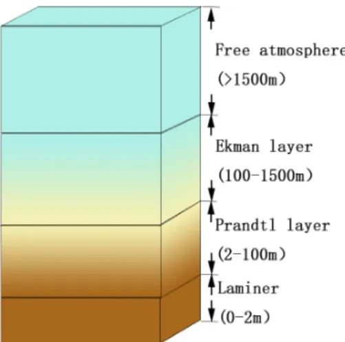
The Earth’s atmosphere can be divided into several layers based on the behaviour of its tem- perature [11], these layers are, starting from ground level upwards, the troposphere, the strato- sphere, the mesosphere and the thermosphere, A further region, beginning about 500 km above the ground level, is the exosphere, which fades away into the realm of interplanetary space. The troposphere contains more than 75% of all of the air in the atmosphere, and almost all of the water vapour (which forms clouds and rain). This is the region where the famil- iar weather phenomena occur. The lowest part-roughly the lower third-of the troposphere is called the atmospheric boundary layer, and it is here that friction plays an important role, while higher up, from the stratosphere upwards, the air flow is practically inviscid.

For a better understanding of the flow dynamics, it is useful to divide the atmospheric boundary layer into there parts [8,11], i.e., the lamina sublayer, surface (Prandtl) layer and

BCorresponding author. Email: jrwang@gzu.edu.cn

the Ekman layer(see Fig. 2.1), the lamina sublayer is only a few millimeters thick and is not relevant to the transfer of wind energy. Within the surface layer, confined to 20–100 meters of the atmosphere (above the lamina sublayer), the velocity profile is adjusted so that the horizontal frictional stress is nearly independent of height. In contrast to this, in the Ekman layer, located on top of the surface layer and extending to a height of about 1 km, on average, the flow is governed by a three-way balance among frictional effects, pressure gradient and the influence of the coriolis force [5,8,21]. Primarily the air flow is horizontal (the horizontal velocities are about 10⁴ larger than the vertical velocity [20]).

The governing equations for mesoscale steady air flow at mid-latitudes in the Ekman layer are [8]

(f(v−vg) =−_∂z^∂(k^∂u_∂z),

f(u−u_g) = _∂z^∂(k^∂v_∂z)_, ^(1.1) where (u,v) represents the horizontal wind velocity, with zonal (West-to-East, in the sense of the Earth’s rotation) componentu=u(t,x,y,z)and meridional (positive meaning towards the North Pole) component v = v(t,x,y,z), u_g and v_g are the corresponding geostrophic wind component, k denotes the eddy viscosity, f = 2Ωsinθ is the Coriolis parameter at the fixed latitudeθ in the Northern Hemisphere andΩ ≈7.29×10⁻⁵s⁻¹ is the angular speed of rotation of the Earth andθ ∈(0,π/2]is the angle of latitude in right-handed rotating spherical coordinates (θ =0 corresponding to the Equator andθ= π/2 to the North Pole).

The boundary conditions for the system (1.1) are

u= v=0 atz=0, (1.2)

and

u→ug, v→vg forz→_∞, (1.3)

expressing the fact that, due to the frictional properties of the flow below the Ekman layer, a no-slip condition holds at the bottomz =0 of the layer, while at the top of the Ekman layer the horizontal components of the wind must be in geostrophic balance: above the Ekman layer the flow is geostrophic (pressure-driven).

Ifkis a constant, then we can obtain the explicit formula of the solution to (1.1) with (1.2) and (1.3) by the classic Ekman theory, but this assumption is too restrictive. The dynamics of the atmospheric boundary-layer is very important in applications, for example, other than meteorology (weather prediction and climate studies), in the control and management of air pollution (since the dispersal of smog in urban environments depends strongly on meteoro- logical conditions) and in agriculture (e.g. dewfall and frost formation). For this reason, it is important, both from the theoretical as well as from the practical point of view, to understand the flow dynamics of the atmospheric boundary-layer in the context of height-dependent eddy viscosities. The available explicit solutions for height-dependent eddy viscosities are very scare, being apparently restricted to special cases, for example, k(z) denote linear and exponentially decaying functions [10,12] or k(z)is a quadratic polynomial [15]. It is remark- able that Constantin and Johnson [2] studied the Atmospheric Ekman flows with variable eddy viscosityk(z) which is a perturbation of the asymptotic and verify the existence of the solution by transforming the Ekman flows into a suitable integral equation and apply iterative technique to give an efficient approach to find the explicit solution, so that for other types of non-constant eddy viscosity we have to rely on case-by-case approximations and numerical simulations [4,6,9,13,14,16].

Remark 1.1. When z = π q2k

f , the wind (u,v) is parallel to and nearly equally to the geostrophic value (u_g,v_g), it is conventional to designate this level as the top of the Ekman layer [8], so we can change the condition (1.3) to

u=ug, v= vg, atz=z0, (1.4)

wherez₀> π q2k

f .

For a constant eddy viscosityk, we can obtain the explicit formula of the solution to (1.1) with (1.2) and (1.3). Based on Remark 1.1, we consider (1.1) with (1.2) and (1.4). The first contribution of this paper is to apply the technique of second linear ODEs (using the notion of sin and cos matrix) to find the explicit solution of (1.1) with (1.2) and (1.4) and give a directly approach to compute the explicit solution.

If we assume the velocity and acceleration at the bottom of the layer are zero, then (1.2) is retained and (1.3) is changed into

u⁰ =0, v⁰ =0 atz=0, (1.5)

so the second aim of this paper is to investigate the explicit solution of (1.1) with (1.2) and (1.5) for an arbitrary height-dependent eddy viscosityk(z). We use the closed form of function series to give the representation of solutions. By using integral change and introducing Green function, a spectrum theorem of a corresponding anti-symmetric compact operator is used to deriving the uniqueness result. Finally, some dynamical properties of solution like asymptotic property, Lyapunov exponents, and stable manifold are characterized.

2 Model description

Motivated by [8], we give the details to derive (1.1) by dividing into four steps.

Step 1. We set up the momentum equation in rotating coordinates.

We derive the relationship between the total derivative of a vector in an inertial reference frame and the corresponding total derivative in a rotating system. Let −→

A be an arbitrary vector whose Cartesian components in an inertial frame given by

−

→A = −→

i⁰ A⁰_x+−→

j⁰ A⁰_y+−→ k⁰A⁰_z

and whose components in a frame rotating with the angular velocity−→ Ω are

−→ A = −→

i Ax+−→

j Ay+−→ k Az, here −→

i ,−→ j ,−→

k are unit vectors which are taken to be directed eastward, northward, and upward, respectively,−→

Ω = (0,Ωsinφ,Ωcosφ),φis the latitude.

Letting ^Dα

−

→A

Dt be the total derivative of−→

A in the inertial frame, we can write D_α−→

A Dt = −→

i⁰ DA⁰_x Dt +−→

j⁰ DA⁰_y Dt +−→

k⁰ DA⁰_z Dt

= −→ i Du

Dt +−→ j Dv

Dt +−→ k Dw

Dt + ^Dα

−→ i

Dt u+ ^Dα

−→ j

Dt v+ ^Dα

−

→k Dt w,

Figure 2.1: Ekman layer, surface layer and lamina sublayer are called the atmo- sphere boundary layer.

the first three terms on the left line above can be combined to give D−→

A Dt =−→

i DAx

Dt +−→ j DAy

Dt +−→ k DAz

Dt , which is just the total derivative of−→

A as viewed in the rotating coordinates. By direct calcu- lation [8], we get

D_α−→ i Dt =−→

Ω×−→

i , D_α−→ j Dt =−→

Ω ×−→

j , D_α−→ k Dt =−→

Ω×−→ k, there, the total derivative for−→

A in an inertial frame is related to that in a rotating frame by D_α−→

A Dt = ^D

−→ A Dt +−→

Ω ×−→

A. (2.1)

For a given air parcel the location (x,y,z) is a given function of t so that x = x(t),y = y(t),z = z(t), let ^Dx_Dt = u,^Dy_Dt = v,^Dz_Dt = w , then u,v,w are the velocity components in the x,y,zdirections, respectively, let−→

U is the velocity vector , then −→ U =−→

i u+−→ j v+−→

k w.

In an inertial reference frame, Newton’s second law of motion may be written as

∑

^{−→F = Dα}

−→ U_α Dt , here ^Dα

−→ Uα

Dt is the rate of change of the absolute velocity Uα. On the rotating Earth, if−→ r is a position vector for an air parcel, from the (2.1), we get

D_α−→ r Dt = ^D

−→ r Dt +−→

Ω × −→ r ,

but ^D_Dt^α−→r = −→

U_α, ^D_Dt^−→r =−→

U, so we obtain

−→ U_α =−→

U +−→ Ω× −→

r . (2.2)

We apply (2.1) to−→

Uα and obtain D_α−→

U_α Dt = ^D

−→ U_α Dt +−→

Ω×−→ U_α. Using (2.2), we get

Dα

−→ Uα

Dt = ^D

−→ Uα

Dt +−→ Ω ×−→

Uα

= ^D Dt(−→

U +−→ Ω× −→

r ) +−→ Ω×(−→

U +−→ Ω × −→

r )

= ^D

−→ U

Dt +2−→ Ω×−→

U −_Ω²−→ R, here −→

R is a vector with direction perpendicular to the axis of rotation, and the magnitude equal to the distance to the axis of rotation.

If we assume that the only real forces acting on the atmosphere are the pressure gradient force−→

F_p , gravitation force−→

F_g and friction force−→

F_r, then we have D−→

U Dt =−→

F_g +−→ F_p+−→

F_r, so we get

D−→ U

Dt =−2−→ Ω ×−→

U +_Ω²−→ R +−→

Fg +−→ Fp+−→

Fr. (2.3)

Step 2. We set up the component equations in spherical coordinates.

Let(_λ,φ,z)be the spherical coordinates, λis longitude,φis latitude, andz is the vertical distance above the surface of the Earth, using the formula for the transformation of local rectangular coordinate system and spherical coordinate system, we can get the following relationships,

dx=acosφdλ, dy=adφ, dz=dr,

where ais the radius of the Earth,r is the distance to the center of the Earth, which is related to zbyr =a+z.

The direction of the −→ i ,−→

j ,−→

k unit vectors are not constant, they are the functions of position on the spherical Earth, thus we write

D−→ U Dt = −→

i Du Dt +−→

j Dv Dt +−→

k Dw

Dt +uD−→ i

Dt +vD−→ j

Dt +wD−→ k

Dt , (2.4)

from [8], we get D−→

i

Dt = ^u

acosφ −→

j sinφ−−→ k cosφ

, D−→ j

Dt = −^utanφ a

−→ i −^v

a

−→

k , (2.5)

and

D−→ k Dt = ^u

a

−→ i +^v

a

−→

j , (2.6)

substituting (2.5) and (2.6) into (2.4) and rearranging the terms, we obtain D−→

U Dt =

Du

Dt − ^uvtanφ

a +^uw

a −→

i + Dv

Dt +^u

2tanφ a + ^vw

a −→

j

+ Dw

Dt − ^u

2+v² a

−→

k . (2.7)

We know that

Ω²−→ R +−→

F_g =−→

g, (2.8)

and

−2−→ Ω×−→

U =−_2Ω







−→ i −→

j −→

k 0 cosφ sinφ

u v w







=−(_2Ωwcosφ−_2Ωvsinφ)−→

i −_2Ωusinφ

−→

j +_2Ωucosφ

−→ k .

(2.9)

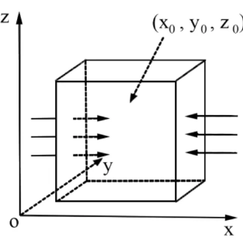
We consider an infinitesimal volume element of air,δV =δxδyδz, center at the point(x0,y0,z0) (see Fig.2.2), so we can easily get the total pressure gradient force per unit mass is

−→ F_p = ¹

ρ∇−→ p =−→

i 1 ρ

∂p

∂x +−→ j 1

ρ

∂P

∂y +−→ k 1

ρ

∂P

∂z, (2.10)

we know that

−→

g =−−→

k g, (2.11)

and

−

→F_r = −→

i F_rx+−→

j F_ry+−→

k F_rz, (2.12)

where











Frx =υ[^∂_∂x^2u₂ + ^∂_∂y^2u₂ + ^∂_∂z^2u₂], F_ry =υ[^∂2v

∂x² +^∂2v

∂y² +^∂2v

∂z²], F_rz =υ[^∂2w

∂x² + ^∂2w

∂y² + ^∂2w

∂z²], υ= ^µ_ρ is the kinematic viscosity coefficient [8].

From (2.3) and using (2.7), (2.8), (2.9), (2.10), (2.11), (2.12), we get the following equations











Du Dt =−¹

ρ 1 cosφ

∂P

∂λ +_2Ωvsinφ−_2Ωwcosφ+^uvtan_a ^φ−^uw_a +F_rx,

Dv Dt = −¹

ρ 1 a∂P

∂φ−_2Ωusinφ−^u2tan_a ^φ −^vw_a +F_ry,

Dw Dt =−¹

ρ

∂P

∂z −g−_2Ωucosφ+^u2+_a^v2 − ^uw_a +F_rz.

(2.13)

Figure 2.2: Thexcomponent of the pressure gradient forcer.

Step 3. We simplify (2.13) in local rectangular coordinates system.

The table 2.1 in [8] shows the terms proportional to ¹_a on the above equations are unim- portant for midlatitude synoptic scale motions, so we omit this terms and get











Du Dt =−¹

ρ

∂P

∂x +2Ωvsinφ−2Ωwcosφ+F_rx,

Dv Dt =−¹

ρ

∂P

∂y −_2Ωusinφ+F_ry,

Dw Dt =−¹

ρ

∂P

∂z −g−_2Ωucosφ+F_rz. Asu= u(t,x,y,z), and ^Dx_Dt =u, ^Dy_Dt =v, ^Dz_Dt =w, we get

Du Dt = ^∂u

∂t + ^∂u

∂x

∂x

∂t + ^∂u

∂y

∂y

∂t + ^∂u

∂z

∂z

∂t = ^∂u

∂t +u∂u

∂x +v∂u

∂y +w∂u

∂z,

Dv

Dt and ^Dw_Dt are similar.

For a wide range of air movements,wu,v[21], so we assumew=0, for the atmosphere below 100km, kinematic viscosity coefficient is negligible except in a thin layer within a few centimeters of the Earth’s surface where the vertical shear is very large [8], soFrx =0, Fry=0 in Ekman layer, as shown in chapter 3 in [8], the magnitude of w can be deduced from knowledge of the horizontal velocityu,v, so we omit the last equation of the system and get

(_Du

Dt = −¹

ρ

∂P

∂x +2Ωvsinφ=−¹

ρ

∂p

∂x+ f v,

Dv Dt =−¹

ρ

∂P

∂y −_2Ωusinφ=−¹

ρ

∂p

∂y − f u.

Step 4. We set up the mean equations.

In a turbulent fluid, a field variable such as velocity measured at a point generally fluctu- ates rapidly in time as eddies of various scales pass the point, so we assume that the field vari- ables can be separated into slowing varying turbulent components, for example, u = u+u⁰, the corresponding means are indicated by overbars and the fluctuating component by primes.

With the aid of the continuity equation

∂u

∂x + ^∂v

∂y +^∂w

∂z =0, and the chain rule of the differentiation, we get

Du Dt = ^∂u

∂t +_u^∂u

∂x +_v^∂u

∂y +_w^∂u

∂z +_u(^∂u

∂x + ^∂v

∂y +^∂w

∂z)

= ^∂u

∂t + ^∂u

2

∂x +^∂uv

∂y +^∂uw

∂z . (2.14)

Separating each dependant variable into mean and fluctuating parts, substituting into (2.14), and averaging then yields

Du Dt = ^∂u

∂t + ^∂

∂x(u u+u⁰u⁰) + ^∂

∂y(u v+u⁰v⁰) + ^∂

∂z(u w+u⁰w⁰). Noting that the mean velocity fields satisfy the continuity equation, we get

Du

Dt = ^{D u} Dt + ^∂

∂x(u⁰u⁰) + ^∂

∂y(u⁰v⁰) + ^∂

∂z(u⁰w⁰), where

D Dt = ^∂

∂t +u ∂

∂x +v ∂

∂y +w ∂

∂z

is the rate of change following the mean motion, the mean equations thus have the following form,

(_Du

Dt =−¹

ρ

∂P

∂x + f v−[^∂u_∂x^0u0 + ^∂u_∂y^0v0 + ^∂u_∂z^0w0],

Dv Dt =−¹

ρ

∂P

∂y − f u−[^∂u_∂x^0v0+ ^∂v_∂y^0v0 +^∂v_∂z^0w0].

Away from region with horizontal inhomogeneities (e.g., shorelines terms, forest edges), we can assume turbulent fluxes are horizontally homogeneous because they are too small in comparison to the term involving vertical differentiation [8], so we assume ^∂u_∂x^0u0 = ^∂u_∂y^0v0 =

∂u⁰v⁰

∂x = ^∂v_∂y^0v0 =0.

Outside the boundary layer, the resulting approximation was geostrophic balance, i.e., (₁

ρ

∂P

∂x = f v_g,

1 ρ

∂P

∂y =−f u_g.

For midlatitude synoptic-scale motions, the inertial acceleration terms (the terms on the left of above equations) can be neglected compared to the Cariolis force and pressure gradient force terms [8], so we get

(f(v−v_g)−^∂u_∂z^0w0 =_0,

−f(u−u_g)− ^∂v_∂z^0w0 =0.

By the Flux-Gradient theory, we get

(u⁰w⁰ =−k(^∂u_∂z), v⁰w⁰ =−k(^∂v_∂z)_,

wherek(_m²_s⁻¹)is the eddy viscosity coefficient, then we have (f(v−v_g) =−_∂z^∂(k^∂u_∂z),

f(u−ug) = _∂z^∂(k^∂v_∂z). Finally, we omit the overbars for simplicity to obtain (1.1).

3 Main results

3.1 Existence of explicit solution

Note that ifkreduces to a constant, then (1.1) reduces to (_d2v

dz² = _k^f(u−u_g),

d²u

dz² =−_k^f(v−vg). (3.1)

Based on Remark1.1, we change the condition (1.3) to (1.4) in the following theorems, and we try to find explicit solution of (3.1) with (1.2) and (1.4) by using the notion of sin and cos matrices.

Definition 3.1 ((see [7]). It is well known that sinΩz= _Ω^z

1!−_Ω^3z

3

3! +· · ·+ (−1)^k_Ω^{2k+1 z}

2k+1

(2k+1)!+· · ·, cosΩz= I−_Ω^2z

2

2! +· · ·+ (−1)^k_Ω^{2k z}

2k

(2k)_!+· · ·.

Theorem 3.2. The solution of (3.1)with(1.2)and(1.4)can be expressed by the following formula v

u

=cosΩz −vg

−u_g

+sinΩz C₂₁

C₂₂

+ vg

u_g

, (3.2)

where

Ω=



 q f

2k − q f

2k

q f 2k

q f 2k



, and

C₂₁ C₂₂

= (_sinΩz₀)⁻¹_cosΩz₀ v_g

u_g

.

Remark 3.3. Note that(sinΩz0)⁻¹does exist becausez₀is a positive number, so usingWolfram Mathematica,(sinΩz0)⁻¹cosΩz0 can be solved by the following computations:

sinΩz₀=



 sin

q f

2kz₀cosh q f

2kz₀ −cos q f

2kz₀sinh q f

2kz₀ cos

q f

2kz₀sinh q f

2kz₀ sin q f

2kz₀cosh q f

2kz₀



, det sinΩz0= ¹

2 cosh 2 r f

2kz₀

!

−cos 2 r f

2kz₀

!!

>0,

(sinΩz₀)⁻¹=











2 sin qf

2kz₀cosh qf

2kz₀ cosh(2

qf

2kz₀)−cos(2 qf

2kz₀)

2 cos( qf

2kz₀)sinh qf

2kz₀ cosh(2

qf

2kz₀)−cos(2 qf

2kz₀) 2 cos

qf 2kz₀sinh

qf 2kz₀ cos(2

qf

2kz0)−cosh(2 qf

2kz0)

2 sin qf

2kz₀cosh qf

2kz₀ cosh(2

qf

2kz0)−cos(2 qf

2kz0)









 ,

and

cosΩz0=



 cos

q f

2kz0cosh q f

2kz0 sin q f

2kz0sinh q f

2kz0

−sin q f

2kz0sinh q f

2kz0 cos q f

2kz0cosh q f

2kz0



, det cosΩz0= ¹

2 cosh 2 r f

2kz0

!

+cos 2 r f

2kz0

!!

>0,

(sinΩz0)⁻¹cosΩz0=











− ^sin(2

qf 2kz0) cos(2

qf

2kz0)−cosh(2 qf

2kz0)

− ^sinh(2

qf 2kz0) cos(2

qf

2kz0)−cosh(2 qf

2kz0) sinh(2

qf 2kz0) cos(2k)−cosh(2

qf 2kz0)

− ^sin(2

qf 2kz0) cos(2

qf

2kz0)−cosh(2 qf

2kz0)









 ,

and

det

(sinΩz0)⁻¹cosΩz0

= cos

2

q f 2kz₀

+cosh

2 q f

2kz₀

cosh

2 q f

2kz₀

−cos

2 q f

2kz₀ >0.

Proof. LetU=u−ug,V =v−vg andk= ^f_k. Then (3.1) becomes (_d2V

dz² =kU,

d²U

dz² =−kV, (3.3)

and the conditions (1.2), (1.4) are transformed into the equivalent forms

U=−ug, V =−vg atz =0, (3.4)

U=0, V =0 atz=z0. (3.5)

From the (3.3), we get

V U

⁰⁰ +

0 −k k 0

V U

=0.

By using the matrixΩ, we obtain V

U 00

+_Ω² V

U

=0. (3.6)

So we get the solution of the (3.6) as following form, V

U

=cosΩz C₁₁

C₁₂

+sinΩz C₂₁

C₂₂

.

We determine the constants such that the initial conditions (3.4) and (3.5) are satisfied. Con- sidering the condition (3.4), we get

C₁₁ =−v_g, C₁₂=−u_g. Considering the condition (3.5), we obtain

0 0

=cosΩz₀ −vg

−u_g

+sinΩz₀ C₂₁

C₂₂

. Because the matrix sinΩz₀ is nonsingular, so we get

C₂₁ C₂₂

= (_sinΩz₀)⁻¹_cosΩz₀ v_g

u_g

. AsU=u−u_g,V =v−v_g, so we obtain (3.2).

We recall the following result.

Lemma 3.4(see [1,18]). For the matrix equation

Φ⁰(t,t₀) = A(t)_Φ(t,t₀), t ∈[t₀,tα]

with the initial boundary condition Φ(t₀,t₀) = I, where the matrix Φ(t,t₀) and A(t) are n×n matrices, t_α >t₀≥0, the solutionΦ(t,t₀)is given by

Φ(t,t₀) =I+

Z _t

t₀ A(τ)dτ+

Z _t

t₀ A(τ₁) _{Z τ}

1

t₀ A(τ₂)dτ₂

dτ₁

+

Z _t

t₀ A(τ₁)

Z _τ1

t₀ A(τ₂)

Z _τ2

t₀ A(τ₃)dτ₃dτ₂dτ₁+· · · For (1.1), we assume thek =k(z)6=0, then we will get







d²v

dz² + ^k_k⁰₍⁽_z^z₎^)dv_dz = _k(^f_z)(u−ug),

d²u

dz² +^k_k⁰₍⁽_z^z₎^)du_dz = −_k(^f_z)(v−vg). Letu−ug=U, v−vg =V, then we will get

(_d2V

dz² +α(z)^dV_dz =β(z)U,

d²U

dz² +α(z)^dU_dz = −β(z)V, whereα(z) = ^k0(z)

k(z), β(z) = ^f

k(z), and the conditions (1.2) and (1.5) will become

U(0) =−u_g, V(0) =−v_g, (3.7) and

U⁰(₀) =_0, V⁰(₀) =_{0. (3.8)}

LetV⁰(z) =w₁, U⁰(z) =w₂, then we obtain

X⁰(z) = A(z)X(z), X(0) =X₀, (3.9) where

X =







 V U W₁ W2









, X₀ =









−vg

−u_g 0 0







 ,

and

A(z) =









0 0 1 0

0 0 0 1

0 β(z) −α(z) 0

−β(z) _{0 0} −α(z)







 .

We get the solution of (3.9) by using Lemma 3.4, that is X(z) =_Φ(z,z₀)X₀, where

Φ(z,z₀) =I+

Z _z

0 A(τ)dτ+

Z _z

0 A(τ₁) _{Z τ}

1

0 A(τ₂)dτ₂

dτ₁+· · ·,

asu−u_g =U,v−v_g =V, so we get the solution of (1.1) with the conditions (1.2) and (1.5).

Ifk(z)is constant, then we will solve (3.9) with the conditions (1.2) and (1.5).

Remark 3.5. Ifk(z)is a constantk, thenα(z) =0,β(z) = _k^f, and (1.1) will become the following form,

X⁰(z) = AX(z), (3.10)

the corresponding initial conditions are

X(0) =X₀, where

A=









0 0 1 0

0 0 0 1

0 β 0 0

−β 0 0 0









. (3.11)

The characteristic equation of (3.11) is

λ⁴+β² =0, so we get the four eigenvalues:

λ₁= r f

2k + r f

2ki, λ₂ =− r f

2k− r f

2ki, λ₃= r f

2k − r f

2ki, λ₄ =− r f

2k + r f

2ki.

Letλ=λ₁, then we have

(A−λ₁I) =









−λ₁ 0 1 0

0 −λ₁ 0 1

0 β −λ₁ 0

−β 0 0 −λ₁







 ,

so the corresponding eigenvector is

ξ₁=













1 i q f

2k + q f

2ki

− q f

2k + q f

2ki











 ,

thus we obtain

e^λ1zξ₁ =e

qf 2kz

























cos q f

2kz+isin q f

2kz

−_sin q f

2kz+icos q f

2kz q f

2k

cos

q f

2kz−sin q f

2kz

+ q f

2k

cos

q f

2kz+sin q f

2kz

i

− q f

2k

cos

q f

2kz+sin q f

2kz

+ q f

2k

cos

q f

2kz−sin q f

2kz

i























 .

The two linear independent solutions are obtained:

X₁(z) =e

qf 2kz

























cos q f

2kz

−sin q f

2kz q f

2k

cos

q f

2kz−sin q f

2kz

− q f

2k

cos

q f

2kz+sin q f

2kz























 ,

and

X₂(z) =e

qf 2kz

























sin q f

2kz cos

q f 2kz q f

2k

cos

q f

2kz+sin q f

2kz q f

2k

cos

q f

2kz−sin q f

2kz























 .

Similarly, letλ₃ =− q f

2k + q f

2ki, we will get the eigenvector

ξ2=

















1

−i

− q f

2k + q f

2ki q f

2k + q f

2ki















 ,

therefore we have

e^λ2zξ₂=e⁻

qf 2kz

























cos q f

2kz+isin q f

2kz sin

q f

2kz−icos q f

2kz

− q f

2k

cos

q f

2kz+sin q f

2kz

+ q f

2k

cos

q f

2kz−sin q f

2kz

i q f

2k

cos

q f

2kz−sin q f

2kz

+ q f

2k

cos

q f

2kz+sin q f

2kz

i























 .

The two linear independent solutions can be stated as follows,

X3(z) =e⁻

qf 2kz























cos q f

2kz sin

q f 2kz

− q f

2k

cos

q f

2kz+_sin q f

2kz q f

2k

cos

q f

2kz−sin q f

2kz





















 ,

and

X₄(z) =e⁻

qf 2kz























sin q f

2kz

−cos q f

2kz q f

2k

cos

q f

2kz−sin q f

2kz q f

2k

cos

q f

2kz+sin q f

2kz





















 .

So the general solution of (3.9) is

X(z) =c₁X₁(z) +c₂X₂(z) +c₃X₃(z) +c₄X₄(z), then

V= c₁e

qf 2kz

cos r f

2kz+c₂e

qf 2kz

sin r f

2kz+c₃e⁻

qf 2kz

cos r f

2kz+c₄e⁻

qf 2kz

sin r f

2kz, (3.12) and

U = −c₁e

qf 2kz

sin r f

2kz+c₂e

qf 2kz

cos r f

2kz +c3e⁻

qf 2kz

sin r f

2kz−c₄e⁻

qf 2kz

cos r f

2kz. (3.13)

By using the conditions (3.7), (3.8), we get c₁ = c₃ = −¹₂vg, c₂ = −¹₂ug, c₄ = ¹₂ug, so the solution of (3.10) with the conditions (3.7), (3.8) is obtained.

Remark 3.6. From the above example, we know that the general solution of (3.10) is (3.12), (3.13), so if we use the traditional boundary conditions (1.2), (1.3), then we will get

c₁= c₂ =_0, c₃=−v_g, c₄ =u_g,

then we have











V=e⁻

qf

2kz

ugsin q f

2kz

−vgcos q f

2kz, U=e⁻

qf 2kz

−vgsin q f

2kz

−ugcos q f

2kz, so the solution is











v= v_g+e⁻

qf 2kz

u_gsin

q f 2kz

−v_gcos q f

2kz, u= u_g+e⁻

qf 2kz

−v_gsin q f

2kz

−u_gcos q f

2kz, this coincides with the result in [8].

3.2 Uniqueness

For the constantk, the explicit solution of (1.1) with (1.2) and (1.4) is obtained by Theorem3.2, in the following theorem, we try to find the uniqueness fork(z).

Theorem 3.7. Assume f 6=0, then there is a unique solution of (1.1)with conditions(1.2)and(1.4).

Proof. Let ˆuand ˆvbe the solutions of (1.1) for f =0 with (1.2) and (1.4). Then ˆ

u(z) = ^l(z)

l(z₀)^{ug, vˆ}(z) = ^l(z) l(z₀)^vg forl(z) =Rz

0 ds

k(s). Thus using in (1.1) the exchange

u↔u+u,ˆ v↔v+v,ˆ we get











f(v+vˆ−v_g) =−_∂z^∂(k(z)^∂u_∂z), f(u+uˆ−ug) = _∂z^∂(k(z)^∂v_∂z), u=v =0 at z=0,z₀.

(3.14) Introducing the corresponding Green function

G(z,s) =







l(s)^l(z)

l(z0)−1

for 0≤s ≤z≤z₀, l(z)^l(s)

l(z0)−1

for 0≤z ≤s≤z₀, (3.14) is rewritten as

(f uˆ (z) =−Rz0

0 G(z,s)(v(s) +vˆ(s)−vg)ds, f vˆ (z) =Rz₀

0 G(z,s)(u(s) +uˆ(s)−u_g)ds (3.15) for ˆf = f⁻¹. Now we consider a Hilbert space H= L²(0,z₀)²with an inner product

((u₁,v₁),(u2,v2)) =

Z _z0

0

(u₁(z)v₁(z) +u2(z)v2(z))dz.

Next introducing a linear operator A: H→ Hby A(u,v)(z) =

_{Z z}

0

0 G(z,s)v(s)ds,−

Z _z0

0 G(z,s)u(s)ds

and functions

˜

u(z) =−

Z _z0

0 G(z,s)(vˆ(s)−vg)ds,

˜ v(z) =

Z _z0

0 G(z,s)(uˆ(s)−u_g)ds, (3.15) is equivalent to

fˆ(u,v) +A(u,v) = (u, ˜˜ v).

Since G(z,s) = G(s,z), it is easy to see that A is anti-symmetric A^∗ = −A. It is also well- known that Ais compact [1,19]. Thus a spectrum of Aconsists from isolated pure imaginary eigenvectors with a limit at the zero and the corresponding eigenvalues form an orthogonal bases of H. Consequently, for any 06= f ∈ _R, there is a unique solution of (3.14), and thus also for (1.1). Some approximations methods can be used for generalk(z)in order to construct these solutions. Ifk(z)is constant then a method presented above is applied.

3.3 Dynamical properties

Conditions (1.2) and (1.5) are Cauchy initial value conditions for (1.1), so they determine a unique solution onR+= [0,∞). We will try to study the uniqueness of (1.1) with conditions (1.2) and (1.3).

Theorem 3.8. For any constant k¯ > 0 there is an e¯ > 0 such that for any continuous function k:R+ →_R+satifying

sup

z∈_R+

|k^¯−k(z)|<e,¯ there is a unique solution of (1.1)with conditions(1.2)and(1.3).

Proof. To study conditions (1.2) and (1.3), we introduce x=k∂u

∂z, y=k∂v

∂z, and (1.1) is replaced by















∂u

∂z =kx,^ˆ

∂v

∂z =ky,^ˆ

∂x

∂z = −f(v−vg),

∂y

∂z = f(u−u_g)

(3.16)

for ˆk = ¹_k. The affine system (3.16) has a unique equilibrium (_{ug,vg, 0, 0})

with the linearization 













∂u

∂z =kx,^ˆ

∂v

∂z =ky,^ˆ

∂x

∂z = −f v,

∂y

∂z = f u.

(3.17)

If sup_z∈R

+

kˆ(z) < ∞, then the asymptotic property of (3.17) is determined by its Lyapunov exponents. When kis a constant function, then the matrix









0 0 kˆ 0 0 0 0 ˆk 0 −f 0 0

f 0 0 0







 has eigenvalues

λ₁= − s

fkˆ

2 (1+i), λ₂=− s

fkˆ

2 (1−i), λ₃ = s

fkˆ

2 (1−i), λ₄ = s

fkˆ 2 (1+i) with the corresponding eigenvectors

−(1+i)

√kˆ

√ 2p

f ,−(1−i)

√kˆ

√ 2p

f ,i, 1

!

, −(1−i)

√ˆk

√ 2p

f ,−(1+i)

√kˆ

√ 2p

f ,−i, 1

! , (1−i)

√kˆ

√ 2p

f ,(1+i)

√kˆ

√ 2p

f ,−i, 1

!

, (1+i)

√kˆ

√ 2p

f ,(1−i)

√kˆ

√ 2p

f ,i, 1

! . So the linear system (3.17) has a stable space

S=









−

√kˆ

√2√

f,−

√kˆ

√2√

f, 0, 1

−

√kˆ

√ 2√

f,

√kˆ

√ 2√

f, 1, 0







 and (3.16) has a stable manifold

W_s= (u_g,v_g, 0, 0) +S.

Thus condition (1.2) holds if [17,18]

(0, 0)∈ (u_g,v_g) +









−

√kˆ

√2√

f,−

√kˆ

√2√

f

−

√kˆ

√2√

f,

√ˆk

√2√

f







 ,

which is uniquely satisfied

(0, 0) = (ug,vg) +c₁ −

√kˆ

√ 2p

f,−

√kˆ

√ 2p

f

!

+c₂ −

√kˆ

√ 2p

f,

√kˆ

√ 2p

f

!

c₁=

√kˆ(ug+vg)

√ 2p

f , c₂ =

√kˆ(ug−vg)

√ 2p

f .

Consequently, there is a unique solution of (1.1) with conditions (1.2) and (1.3). This is already shown above in Remark3.6. By using a roughness result [3, Proposition 1, p. 34], we see that for any constant ¯k > 0 there is an ¯e> 0 such that for any continuous function k :R+ → _R+

such that

sup

z∈_R+

|k^¯−k(z)|<e,¯

there is a unique solution of (1.1) with conditions (1.2) and (1.3). ¯e can be estimated in the term of ¯k and f, but we do not go into details. Sincek(z)is just continuous, here we have a solutionu(z),v(z)of (1.1) such thatu(z),v(z), ^∂u_∂z^(z), ^∂v_∂z^(z), _∂z^∂(k(z)^∂u_∂z^(z))and _∂z^∂(k(z)^∂u_∂z^(z))exist and continuous onR+. The proof is complete.

Acknowledgements

The authors are grateful to the referees for their careful reading of the manuscript and their valuable comments. We also thank the editor.

This work is partially supported by the National Natural Science Foundation of China (11661016), Training Object of High Level and Innovative Talents of Guizhou Province ((2016)4006), Department of Science and Technology of Guizhou Province (Fundamental Re- search Program [2018]1118), Guizhou Data Driven Modeling Learning and Optimization In- novation Team ([2020]5016), the Slovak Research and Development Agency under the contract No. APVV-18-0308, and the Slovak Grant Agency VEGA No. 1/0358/20 and No. 2/0127/20.

References

[1] C. Chicone, Ordinary differential equations with applications, Springer-Verlag, New York, 2006.https://doi.org/10.1007/0-387-35794-7;MR2224508

[2] A. Constantin, R. S. Johnson, Atmospheric Ekman flows with variable eddy viscos- ity,Boundary-Layer Meteorol.170(2019), 395–414.https://doi.org/10.1007/s10546-018- 0404-0

[3] W. A. Coppel, Dichotomies in stability theory, Springer-Verlag, Berlin, 1978.https://doi.

org/10.1007/BFb0067780;MR0481196

[4] Y. Du, R. Rotumno, A simple analytical model of the nocturnal low-level jet over the great plains of the United States,J. Atmos. Sci.71(2014), 3674–3683.https://doi.org/10.

1175/JAS-D-14-0060.1

[5] V. W. Ekman, On the influence of the earth’s rotation on ocean-currents, Ark. Mat. Astr.

Fys.2(1905), 1–52.

[6] B. Gayen, S. Sarkar, J. R. Taylor, Large eddy simulation of oscillating boundary layer under an oscillatory current, J. Fluid Mech. 643(2010), 233–266. https://doi.org/10.

1017/S002211200999200X

[7] N. J. Higham, Functions of matrices: theory and computation, Society for Industrial and Applied Mathematics, Philadelphia, 2008.https://doi.org/10.1137/1.9780898717778;

MR2396439

[8] J. R. Holton,An introduction to dynamic meteorology, Academic Press, New York, 2004.

[9] C. T. Hsu, X. Y. Lu, M. K. Kwan, LES and RANS studies of oscillating flows over flat plate, J. Eng. Mech. 126(2000), 186–193. https://doi.org/10.1061/(ASCE)0733- 9399(2000)126:2(186)

[10] O. S. Madsen, A realistic model of the wind-induced boundary layer, J. Atmos.

Sci. 7(1977), 248–255. https://doi.org/10.1175/1520-0485(1977)007<0248:ARMOTW>2.

0.CO;2

[11] J. Marshall, R. A. Plumb, Atmosphere ocean and climate dynamic: an introduction text, Academic Press, New York, 2016.