M O D E L R E F E R E N C E A D A P T I V E S Y S T E M S T O I M P R O V E R E L I A B I L I T Y
H. P. Whitaker and Allen Kezer Department of Aeronautics and Astronautics,
Massachusetts Institute of Technology, Cambridge, M a s s . A B S T R A C T
One m e a n s for improving the reliability of an automatic control system is proposed whereby the system is given the capability for reorganizing or readjusting itself to repair the effects of failure of the components of the system. This paper shows how a model reference adaptive control system can be used to realize that capability, and shows by simula- tion of the performance of an aircraft flight control system how the rapid convergence times of these systems can ac- complish the necessary readjustments fast enough to prevent dangerous flight disturbances due to the failures. Extension to other flight vehicles can be readily m a d e .
I N T R O D U C T I O N
The purpose of this paper is to describe the use of a model reference adaptive control system not only to achieve a specified dynamic performance but also to increase con- trol system reliability. It is an extension of the work re- ported in Refs. 1 and 2 to the consideration of providing a capability for self-reorganization after partial failure occurs.
Presented at A R S Guidance, Control, and Navigation Conference, Stanford, Calif., Aug. 7-9, 1961. The research leading to this paper w a s carried out under the auspices of the Massachusetts Institute of Technology D S R Project 52-156, sponsored by the Ballistic Missile Division of the Air Research and Development C o m m a n d through U S A F Contract A F 04(647)-303.
^"Associate Professor.
2Staff M e m b e r .
Adaptive control systems have been developed so that a specified dynamic performance can be achieved, even though the characteristics that affect that performance vary during the operating times of the system due to either
changes in environment or wholly unanticipated reasons.
The mission of a high performance aircraft provides ex- amples of the former, and this paper considers various failures of typical components in a system as examples of the latter. B y using an adaptive system combined with re- dundant control channels, acceptable performance can result even though certain multiple failures occur. The model reference adaptive system is attractive for this application because of its rapid convergence to the optimum operating condition from an arbitrary initial state. The parameters can be readjusted fast enough to prevent dangerous flight attitudes even in the event that a failure occurs which would cause instability if no adaptation took place.
Since the emphasis of this paper is on the use of an adaptive system, it is not the authors1 purpose to present an exhaustive treatment of the hardware considerations in the design of redundant channels for reliability. A n auto- matic control system for aircraft will be used as an example to illustrate the techniques, but other control applications can of course be suggested.
M O D E L R E F E R E N C E A D A P T I V E S Y S T E M S
3
The model reference adaptive control concept (1-4), as originally proposed and investigated at the M , I. T. Instru- mentation Laboratory, w a s evolved to m a k e it possible to design a control system that could adjust its own controllable parameters so that its dynamic performance would satisfy the system specifications in the presence of changing operat- ing characteristics. T o do this, a reference model is pro- vided which stores the system specifications and permits closed loop control of the parameters through the use of response error functions measured during the normal oper- ating responses of the system. Optimum, or fully adapted, performance is achieved when the measured error functions have values corresponding to a specified performance index.
Use of the model permits design flexibility, since the model can change with the operating m o d e s of the vehicle and can exhibit nonlinear characteristics if the system specifica- tions require these features.
N u m b e r s in parentheses indicate References at end of paper.
Fig. 1 is a simplified functional diagram of the adaptive system. The dotted box encloses the components that are contained in a complete closed loop control system capable of performing its assigned function provided its parameters can be adjusted to proper values. The input to the system is also fed to a reference model, the output of which is pro- portional to the desired response. This output is compared with the indicated system output to form the response error.
The need for parameter adjustments is determined by gen- erating functions of the error, and c o m m a n d signals calling for time rates of change of the controllable parameters are sent to the parameter adjustment devices in the control sys- tem. A n y needed parameter adjustment takes place when- ever any typical operating input signal or disturbances exist, and the adaptive features can be operated continuously. N o special test inputs (step function, impulses, sinusoids, etc.) are needed.
The model reference adaptive control concept can readily be applied to m a k e any control system adaptive by using the design techniques described in Ref. 2 and in the Appendix. The dynamic performance of the control system will then approximate that of the reference model, whose output is proportional to a system output that meets the sys- tem specifications. The controllable loop parameters are adjusted automatically so that the integral squared error between the system and model outputs is minimized, which is accomplished by nulling an integral error quantity for each parameter, as shown in the Appendix. A s a result, convergence times on the order of the dominant character- istic time of the system can be obtained, and the adaptive features can be mechanized with simple equipment. The concept has been successfully applied to higher order sys- tems with several controllable parameters and to cases with nonlinear or variable models.
U S E O F R E D U N D A N T C H A N N E L S
The possibilities for improving the overall probability of mission success through duplicating or triplicating a flight control system with independent control channels have been extensively discussed in the literature (5, 6). Redun-
dancy techniques rely on the fact that the probability of complete failure of the system to perform satisfactorily can be m a d e less than the probability of failure of a single
channel. This paper uses as an example an aircraft multi- loop control system that is triplicated to provide a three- fold independent redundancy. B y proper selection of the
design output capability of each channel, one entire channel
can fail completely, and the original dynamic performance can still be achieved. One channel overcomes the effects of the failed channel, and the third channel remains to provide the required control capability. A triplicated system also m a k e s it possible to determine which channel has failed so that it can be deactivated. If, in addition, the failure causes a change in dynamic characteristics, an adaptive capability can restore the original dynamic response.
In an aircraft that must use a fully powered hydraulic actuator to deflect a control surface, the pilot mechanically controls the position of the servo valve, and reliability is achieved by duplicating the hydraulic systems and providing emergency sources of power. To provide automatic control, smaller servo actuators are used to add inputs to the main hydraulic actuators either in parallel with or in series to those of the pilot, as shown in Fig. 2. If redundant auto- matic control channels are provided, the outputs of the several servo actuators must be s u m m e d mechanically in s o m e manner and then fed into the main actuator. T w o methods are generally considered. In one, the output m e m - ber shafts of the servo actuators are tied in parallel to a
c o m m o n linkage m e m b e r , which in effect s u m s the force outputs of the actuators to cause a resultant m o v e m e n t of the linkage m e m b e r . In the other method, a series mechan- ical s u m m i n g linkage is used to obtain a mechanical dis- placement of some point proportional to the sum of the individual displacements of the actuator output shafts. In a multiloop system that is adaptive, the series summation design can also compensate for certain secondary failures in addition to one servo actuator failure without any reduc- tion in system performance, and certain tertiary failures can occur with only a resulting reduced output operation.
There is an analogy here with the case of a loss of an engine on a multi-engine aircraft for which the remaining power permits safe operation although with a reduced m a x i m u m performance. One disadvantage of the series method is that a loss of one of the channels results in a reduction of loop gain with a corresponding change in dynamic performance, but the adaptive system removes this limitation in the s a m e
manner that it handles loop gain changes due to changes in environment. T o illustrate these adaptive features, the series summation method w a s selected as an example for this paper. There are other advantages of each method, but these need not be considered here.
M a n y failures in the various components m a y be classed as either "hard-over" failures or "open circuit" failures.
The net result of the first type is that a servo actuator drives
at its m a x i m u m speed in one direction, which m a y be caused by any failure that holds a valve wide open. In the second type there is an abrupt loss of signal in one channel with an attendant loss in the overall system loop gain. Other failures due to slow deterioration or intermittent operation m a y also occur, but these are not as critical from the flight safety viewpoint.
I L L U S T R A T I V E E X A M P L E
Consider the yaw control system of Figs. 3a and 3b for controlling the lateral axes (roll and yaw) of a supersonic transport (7). This particular control system has been chosen so that the adaptive techniques could be illustrated using a system whose dominant linear dynamic character- istics were at least fifth order, and which required the ad- justment of three controllable parameters to satisfy its per- formance index. The input c o m m a n d to the system applies a torque about the output axis of a single degree of freedom integrating gyro unit, and the resulting control action causes the aircraft to rotate so that there is a component of its angular velocity with respect to inertial space about the air- craft yaw axis proportional to the input c o m m a n d . With no c o m m a n d , the aircraft maintains a constant yaw orientation with zero roll angle. Roll rate and roll angle loops are also provided for stability. Further description of this type of system can be found in Ref. 3.
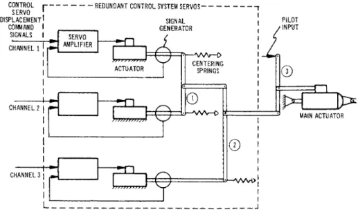
The systems and aircraft of Fig. 3 were simulated on a G P S repetitive, compressed time analog computer. Three redundant channels were provided, and the output displace- ments of the three autopilot servos were mechanically s u m m e d by an arrangement that can be drawn schematically as in Fig. 4, in which the three hydraulic autopilot servos are shown. Linkage m e m b e r s 1 and 2 were floating s u m m i n g m e m b e r s . Each servo w a s loaded by preloaded springs so that a disengaged servo would provide a pivot point for its corresponding floating linkage m e m b e r . In normal opera- tions, however, the displacements of the three servos would be approximately equal, and the s u m m i n g m e m b e r s would translate only. In case of failures that permitted release of hydraulic pressure in the failed channel, the spring restraints would recenter the servo. Floating m e m b e r 3 added the ser- vo outputs in series with those of the pilot, and the springs had to provide preloads greater than the value reaction forces so that this m e m b e r would rotate when the servos were disengaged.
To m a k e the system adaptive, three system parameters were controlled to obtain optimum performance throughout the flight profile of the aircraft. These were taken to be the open loop gains of the three feedback loops of Fig. 3. To achieve the s a m e type of failure protection that w a s provided in the triplicated basic control system, the adaptive system w a s also triplicated. Since it is desired that the magnitudes of the input signal to the three servo actuators be equal to prevent spurious disengagements, any variation in gain called for by one adaptive system varied the gains of all three sys- tems. This w a s equivalent to mounting three potentiometers on the s a m e servo driven shaft, although in practice variable gain gates driven by an electronic counter would be used.
Because the adaptive equipment w a s triplicated, there would be three sets of gates for each of the variable parameters.
For simplicity, in Fig. 3 only one of the redundant con- trol system channels is shown. With the exception of the main actuator and the aircraft, the components would appear in triplicate. The three control servos and the tie-in to the main actuator would appear as shown in Fig. 4. Similarly, only one channel of adaptive equipment is shown to control the three variable gain gates, G^, G^, G^. Each set of gates changes the corresponding gains of the three redundant channels, as shown schematically for gate G^. Such" an amount of equipment would be impractical in an aircraft in- stallation a few years ago before the development of modern computer technology. N o w , the packaging of this amount of capability can be relatively small and simple in comparison with m a n y current systems. For purposes of notation, the three controllable system parameters were designated as follows: P^, the open loop gain of the yaw integrating gyro loop; P^. the ratio of the roll angle stabilization loop gain to P^; and P^, the ratio of the roll rate damping loop gain to P^.
Provision w a s m a d e for monitoring a failed channel so that it could be deactivated. W h e n this took place, the dis-
engaged servo w a s recentered by the centering springs with a longer characteristic time constant than that of the engaged servo. The monitor compared the output displace- ment of the three autopilot servos and disengaged one if its output w a s not the same as those of the other two within a given tolerance level. Since the system is nonlinear, a simulation scale factor must be specified when discussing the nonlinear elements. With the selected scale factor, the monitor level used corresponded to 6 6 % of full travel of one
series actuator. This is m u c h higher than necessary for providing reasonable protection against nuisance disengage- ments. The logic for the monitor is summarized in the following equations:
c o m m a n d to disengage channel 1, 2, 3 autopilot actuator displacements of channels 1, 2, 3
tolerance level (positive)
(!δ1 - δ2ί > e ) and ( |δχ - δ | > e ) = ab ( I δ χ - δ 21 > e ) and ( |δ 2 - δ 3 | > € ) = ac
- δ3| > € ) and ( | δ2 - δ3Ι > € ) = be A failure anywhere in a channel disengaged that channel if the outputs were sufficiently different. Upon disengaging one channel, no further automatic monitoring action took place, but an indication of the failure w a s presented to the pilot so that he would be aware of his reduced system capa- bility and could take appropriate emergency procedures.
Typical results are shown in Figs. 5-7. Fig. 5 is pre- sented to show the capability of the adaptive system to con- verge rapidly to its optimum state from an arbitrary set of the parameter values. At zero time, w a s 5 7 % of its optimum value, P2 w a s 7 0 % and P^ w a s 57%. Such a mis- match of parameter values would be extremely unlikely even at the time the control system is first activated, although a multiple failure can be visualized which would correspond to this case. The input to the system w a s a step function c o m m a n d applied at zero time, calling for a constant bank angle turn followed by a step function roll-out c o m m a n d applied after the roll-in had been completed. Fig. 5a shows the desired yaw angular velocity (or roll angle) response as represented by the output of the model. Superimposed on the model is the response of the system with the adaptive
system operating to readjust the parameters. The response error w a s reduced to and remained less than 5 % of the steady- state input c o m m a n d in a time that is roughly 4 0 % greater than the model1 s response time. Fig. 5b shows that the major readjustment of the parameters took place using only the error information available during the first transient
maneuver. Fig. 5c shows that had no adaptation taken place, A , B , C
δ1 ' δ2 ' δ3
e A B C
the system would be only marginally stable and quite un- usable. To experience this gain configuration through sys- tem failures, an approximately equivalent case results if one channel fails and is disengaged, if there has been an
"open" in one of the remaining channels, and if there has been an "open" in one of the remaining P^ channels.
Fig. 6 shows the operation of the system when a "hard- over" failure occurs during level flight with no input c o m - mand. Fig. 6a is with no monitoring action, and Fig. 6b is with monitoring action and recentering of the failed channel.
In each case a 3 3 % reduction in loop gain results. In the absence of an input c o m m a n d , the disturbance resulting from the failed servo appeared to the adaptive system as an output m e m b e r disturbance, but even this provided s o m e information for gain readjustment. The speed of adaptation is dependent on the gain of the adaptive loop and the m a g - nitude of the error signal. For the conditions of this run P^
achieved approximately 2 5 % recovery during the transient caused by the "hard-over" failure. The primary adjustment required w a s that of P^, although all gains adjusted them- selves in an attempt to minimize the disturbance.
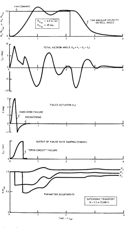
Fig. 7a shows the operation of the system for a c o m - pound failure occurring during the transient response to an input c o m m a n d . The sequence of events of this run was: 1) a c o m m a n d to the system at t = 0; 2) a "hard-over" failure at t Ar ef = 0· 18; 3) detection of the failure and recentering of the failed channel; and 4) open in one of the two remaining rate damping paths at
^J^
ref ~
0. 45. These failures caused a 3 3 % reduction in P^ followed by a 5 0 % reduction in P^. It can be seen from Fig. 7b that with no adaptation this c o m - pound failure resulted in an almost unstable system that rendered it unusable. With the adaptive system operating, the system not only retained good stability, but the adapta- tion restored the original dynamic performance in a time interval following the failures of approximately 1. 3 times the response time of the model. Only the m a x i m u m output level has been reduced due to the loss in servo output capa- bility.S U M M A R Y
The results of the simulation study presented in this paper show that model reference adaptive control techniques
further extend the improvements in system reliability which can be obtained by using redundant control channels. Because of rapid convergence to the optimum operating condition, the adaptive system can readjust system parameters to prevent instability, even though failures cause abrupt changes in sys- tem characteristics which could result in instability if no adaptation takes place. Although the system m a y m o m e n t a r - ily be unstable after a failure or a series of failures, the parameters can be readjusted fast enough to prevent an ex- cessive perturbation of the system output.
The example that w a s chosen to illustrate the basic principles is an aircraft flight control system, but the s a m e techniques m a y be applied to m a n y control problems. These techniques should be of particular interest in automatic land- ing of commercial aircraft where reliability must be ex- tremely high and in the control of satellites and outer space probes where the extremely long times of flight indicate a fairly low probability of successful completion of a mission when using single channel systems.
The following considerations are pertinent to the design of model reference adaptive systems:
1) The concepts can be applied to any control system whose parameters must be varied during its operating time in order to achieve a specified dynamic performance.
2) Adaptation can take place continuously using the normal operating and disturbance inputs to the system.
3) N o special test inputs are required.
4) Error quantities required for adjusting the param- eters can be readily generated using signals available in the control system.
5) The model is designed by the system specifications and need only approximate the dynamic characteristics of the system over the frequency range of importance.
6) The filters required to generate error weighting functions are specified by the model design and the fixed compensation elements of the control system.
7) The system is sensitive to instability and will rapidly readjust parameters to avoid instability.
8) W h e n used in conjunction with redundant channels, it permits safe operation even with multiple component failures.
A P P E N D I X
This appendix describes the analytical considerations for design of model reference adaptive control systems. A
m o r e complete discussion appears in Refs. 1 and 2.
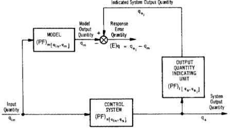
F o r the purpose of definition of t e r m s , Fig. 8 is a mathematical block d i a g r a m representation of the m o d e l reference adaptive system of Fig. 1, showing the generation of the response error quantity. T h e p e r f o r m a n c e of each c o m p o n e n t block of the d i a g r a m is represented b y its per- f o r m a n c e function (or transfer function) with subscripts that identify the c o m p o n e n t and its input and output quantities.
T h e criterion for successful adaptation is that the inte- gral squared error b e the m i n i m u m value obtainable with the p a r a m e t e r variation provided. T h e response error is the difference b e t w e e n the system output and the m o d e l output quantities. T h e p e r f o r m a n c e index is thus given b y
/ ( E ) 2 dt = / ( qe. - qm) 2 dt = minimum [ A - l ]
Since (E) = f (Ρ-, P9, . . . Ρ , t), w h e r e the Ρ are the
χ η η controllable loop p a r a m e t e r s , the desired operating state
for the system is the one at which
- ^ - ( / ( E ) 2 d t ) = 0 [A-2]
If the limits of integration are independent of Pn and if the integral of the derivative of the function exists, an error quantity can b e defined b y
( E C ) P n = / ^ d t = 2 / ( ^ - ) E d t [ A - 3 ]
T h e p e r f o r m a n c e index then requires that this error quantity b e zero. E q . A- 3 states that if an error quantity signal could b e generated proportional to the product (the rate of change of the error with the p a r a m e t e r multiplied b y the error), the p a r a m e t e r should b e adjusted until the integral of that signal is zero. In practice, the integration can b e p e r f o r m e d b y the s a m e device that adjusts the p a r a m e t e r , and it is re- quired only to generate the product of the two signals and feed this quantity as a n input signal to the p a r a m e t e r adjust- m e n t device. T h e net change in the p a r a m e t e r over s o m e time interval is then proportional to the integral error function. That is
A Pn= ( E Q ) Pn [A-4]
The net change in the parameter is zero when the error quantity is nulled.
The error quantity function of Eq. A-3 can be expressed in an alternative manner by interpreting (8Ε/θΡ ) as an error weighting function W-^it), or
where C is an arbitrary constant.
Ref. 2 shows that this weighting function can be readily generated in a model reference adaptive control system as follows. Because variations in the system parameters do not affect the model
Since q . is the only indication of the system output quantity, si
no loss in generality occurs if the subscript i is dropped.
The determination of W^(t) = O q / 8P ) can be accom-
sLt s η
plished in two ways. In one of these, a straightforward partial differentiation of the differential equation for q as
s a function of the input quantities can be m a d e . A n alterna- tive method leads m o r e directly to the system signals that are needed for generating the weighting function. If the sys- tem mechanization is considered, the controllable param- eter can always be represented as a variable sensitivity S in s o m e signal path of the system. This is true even if ^ the effect of the change in the sensitivity is to change a c o m - pensation time constant rather than a control loop gain. The partial derivative (9 cis/9Pn) *s proportional to the change in the system output for a change in the sensitivity. The variable sensitivity for a typical case can be represented as shown in Fig. 9. Across the controllable sensitivity
( E Q ) Pn = C / WE( t ) E ( t ) dt [A-5]
[A-6]
eS - Sp e2 [ A- 7 ] Also
3 es - e2 BSp; es + B es - Sp e2 + e2 3 Sp [ A- 8 ]
The effect of the change 8S can be considered as a disturb - ance entering the system at a point following S^. Ref. 8 shows Ρ 2 that the performance function relating the output of the system 8 qg to a disturbance input is equal to the performance function of the system for the q^n input multiplied by the reciprocal of the performance function of the chain of components of the forward signal path from the input q. to the disturbance summation point, or
^= ( P F )S^ i ni qs] ( l P F T 7 7 r)e2 ^ P [ A" 9 ] Hence
(^") =(PF* f < W q , ] ( ( P F ) , . . . )) 62 IA " 101
Eq. A-10 shows that the error weighting function is a quan- tity that could be generated by taking the signal that occurs at the input to the variable parameter and feeding it through a filter having the s a m e performance function as the system, cascaded with a filter that is the reciprocal of s o m e of the forward path components. However, the first filter cannot be used, because it is exactly this ignorance of the system that leads to the requirement for adaptation.
The model reference system provides a w a y out of this dilemma by the inherent requirement that the model is de- signed so that it provides a good approximation to the dy- namic characteristics of the system when the P*s are
properly adjusted. Thus the approximation to Eq. A-10 is m a d e by substituting the model performance function for that of the system. The Laplace transform of the error weighting function then is
WEW =<P F> m [ qi n, qm] ( ( p^ T T ) ^ W
In practice, the controllable sensitivities can be located at points for which the cascaded forwarded loop performance functions are constant or at most simple known compensa- tion functions.
Other equivalents for different configurations are readily drawn.
N O M E N C L A T U R E
^ X ~r o^ a nS-'-e
C = arbitrary constant
= response error defined as difference b e t w e e n the m o d e l and the s y s t e m output
quantities
e = control path voltage signal
( E Q ) p = error quantity for the p a r a m e t e r P; a function of the error w h i c h indicates the need for adjustment of Ρ
G = variable gain gates for p a r a m e t e r adjustments
Ρ = value of a controllable s y s t e m p a r a m e t e r Δ Ρ = incremental adjustment to Ρ
( P F ) r -, = p e r f o r m a n c e function of c o m p o n e n t η
nl Qj_n^ Qoui* relating the output QQU^ to the input q^
cjin = system input quantity
= m o d e l output quantity qg = system output quantity
q = indicated s y s t e m output quantity s ·
1
S r -, = static sensitivity of c o m p o n e n t η relating
nL <lj_n> ^outJ the output <iQ ^ "to the input q^ under steady conditions
t = time
t „ = reference time to normalize time response
r e records (t f = response time of the m o d e l to a step-input)
Wg(t) = error weighting function
W^= aircraft roll angular velocity with respect to inertial space
= aircraft y a w angular velocity with respect to inertial space
δ aircraft aileron deflection a
δ 1,2,3 autopilot actuator outputs of channels 1,2,3
€ = tolerance level of the monitor λ = Laplace operator
τ = time constant of c o m p o n e n t identified b y subscript
ζ = d a m p i n g ratio (fraction of critical) ω = natural frequency
A = aircraft
as = autopilot servo m s = m a i n servo
S = output of a variable sensitivity point ss = steady state
s = system i = indicated m - m o d e l
R E F E R E N C E S
1 O s b u r n , P. V . , S c D . Thesis, Dept. of Aeronautics and Astronautics, Massachusetts Institute of Technology, Instrumentation Laboratory Report T - 2 6 6 , S e p t e m b e r 1961.
2 O s b u r n , P. V . , Whitaker, Η . P. , and K e z e r , Α . ,
" N e w development in the design of model-reference- adaptive control s y s t e m s , " Institute of the A e r o s p a c e Sciences P a p e r N o . 61-39, Jan., 1961.
3 Whitaker, Η . P. , Y a m r o n , J. , and K e z e r , A . ,
"Design of model-reference-adaptive control s y s t e m s for aircraft," Rept, R - 1 6 4 , Instrumentation L a b . , M a s s . Instit.
Technology, Sept. 1958.
Subscripts
1,2,3, . . arbitrary c o m p o n e n t s c c o m m a n d
4 W h i t a k e r , Η . P., " A n adaptive s y s t e m for control of the d y n a m i c p e r f o r m a n c e of aircraft and spacecraft, " Instit.
Aeronautical Sciences, P a p e r no. 59-100, June 1959.
5 Fearnside, Κ . , "Instrumental and automatic control for approach and landing," J. Inst. Navigation 7, no. 1, Royal Geographical Society, L o n d o n , Jan. 1959,
6 H o w a r d , R . W . , Borltrop, R . K . , Bishop, G . S . , B e v a n , F , , "Reliability in automatic landing, " Flight, Illiffe Transport Publications Ltd. Dorset H o u s e , L o n d o n , Oct. 7, 1960.
7 Stone, R . W . , Jr., "Flying qualitites of supersonic transports," in T h e Supersonic Transport - A Technical S u m m a r y , T e c h . Note D - 4 2 3 , N A S A , June 1960.
8 Truxal, J.G. , Control S y s t e m Synthesis ( M c G r a w - Hill B o o k C o . , Inc., N e w Y o r k , 1955).
Indicated Output Quantity Signal
Reference Settings
Signal Parameter Variation Commands
Γ "
Directional Control Commands
Interference _ Forces and Torques
in.
STABILIZATION AND DIRECTIONAL
CONTROL SYSTEM
Elevator Angle Aileron Angle Rudder
Angle PERFORMANCE
REFERENCE MODEL
ERROR SIGNAL
Response
Error PERFORMANCE
OUTPUT QUANTITY PERFORMANCE
REFERENCE MODEL
ERROR
SIGNAL ANALYZER INDICATING
PERFORMANCE REFERENCE
MODEL Model Output
COMPARATOR UNIT
AIRCRAFT
Π
Aircraft Output Quantities
Basic Flight Control System I
1 Simplified functional d i a g r a m for a m o d e l reference adaptive flight control system
AUTOMATIC CONTROL
PILOT MECHANICAL
INPUT
FOR PARALLEL OPERATION: POINT A IS A FIXED PIVOT FOR ROTATION.
FOR SERIES OPERATION: POÎNT A IS FREE TO MOVE (suitable reaction forces assumed)
. 2 Schematic diagram for providing automatic control deflection of an aircraft control surface
CO
• i H
γ-ι ι
t 'sec
c d TS
CD LO 1.0 s
—* CD
U Ii II II
II MODE
h5 S
! AN SPORT rad/sec rad
CTF CD
INOS sec sec
jper:
c d CD χ
I
to CD
χ
1!
<• .<
- 1 = , °
CO >
Co
or Do
CO >
< c ζ :
-< +
ο ο — +
+
α )
,ΰ αϊ
Χ! 0
•+-»
Ο ε 2 ε
^ ΓΗ
3 - g
r H Ο
CÖ ο
. ΗΗ ° 1 ϋ
CD · Η η -Μ
0) Cd
ω
• Η Η Ο
CO
• Η
c e > - ο
< t ^ ζ
< c = 3 ο ^ rv
< c > ο
CONTROL ρ - REDUNDANT CONTROL SYSTEM SERVOS-
Fig. 4 Schematic diagram of three redundant servos whose output displacements are added mechanically
. YAW ANGULAR VELOCITY OR ROLL ANGLE
1 2 3 (o) Model ond yaw angulor velocity during first solution with adoptive system operating
_L
1 2 3 (b) Parameter adjustments during first solution with adaptive system operating
SUPERSONIC TRANSPORT
YAW / \ M = 3.5 at 75,000 ft.
COMMAND / \
* / \ A \ / YAW ANGULAR VELOCITY
\y OR ROLL ANGLE
\ 1 /
TIME - t / tr ef
(c) System response with no adaptation
ig. 5 Typical operation of the adaptive y a w orientation control system with the loop gains offset f r o m o p t i m u m
P, PARAMETER ADJUSTMENT
FAILED ACTUATOR ( 5 , )
2 0 TIME - t / tr ef
(o) Hard-over foi lure with no monitoring action - oaaptive system operating.
(b) Hard-over failure with monitoring and recentering of failed channel - adaptive system operating.
F i g . 6 O p e r a t i o n of t h e a d a p t i v e y a w orientation s y s t e m in the e v e n t of a h a r d o v e r failure a n d n o input c o m m a n d
Fig. 7a Operation of the adaptive yaw orientation control system in the event of a compound failure during the response to an input c o m m a n d ; adaptive system operating
YAW C O M M A N D
YAW A N G U L A R V E L O C I T Y OR R O L L A N G L E
0 1 2 3
T I M E - t / tr ef
7b Response of the yaw orientation control system in the event of a compound failure during the response to an input c o m m a n d ; no adaptation
Input Quantity
Indicated System Output Quantity
Model Output MODEL Quantity
( Ρ« " [ * Ι π ' * . η ] Ρ )
Response . Error
v Quantity ( E ) q = q , . - qm
OUTPUT QUANTITY INDICATING
UNIT
(
ρρ).[,..,.,]
CONTROL SYSTEM
System Output Quantity
Fig. 8 Mathematical block diagram representation of a model reference adaptive control system
e2d Sp
( P F ) , (PF), ( P F )4
^ ' S o U ^ - I( P F ) ,
Fig. 9 Generalized control system block diagram