Ensembles of Fuzzy Cognitive Map Classifiers Based on Quantum Computation

Ensembles of Fuzzy Cognitive Map Classifiers Based on Quantum Computation

Nan Ma

¹

, Hamido Fujita

²

, Yun Zhai

³

, Shupeng Wang

⁴

1College of Information Technology, Beijing Union University, Beisihuan East 97, 100101 Beijing, China, xxtmanan@buu.edu.cn

2Iwate Prefectural University, Takizawa Sugo 152, 020-0693 Iwate, Japan, hfujita-799@acm.org

3E-Government Research Center, Chinese Academy of Governance, Changchunqiao 6, 100089 Beijing, China, yunfei_2001_1@aliyun.com

4Institute of Information Engineering, China Academy of Sciences, minzhuang 89, 100093 Beijing, China, wangshupeng@iie.ac.cn

Abstract: Fuzzy cognitive maps (FCMs) have been widely employed in the dynamic simulation and analysis in the complex systems. While a novel classifier model based on FCMs （FCMCM）was proposed in our former work, the obvious bottleneck of the genetic leaning algorithm used in FCMCM is its irksome efficiency, in particular, low speed in cross over and mutation delay in global convergence. Moreover the lack of the necessary robustness of a single FCMCM limits its generalization. To this end, a quantum computation based ensemble method FCMCM_QC is proposed to address the scalability problem, which employs a novel evolutionary algorithm inspired by quantum computation.

The FCMCM_QC effectively uses the concept and principle of quantum computation to facilitate the computational complexity of genetic optimization for the FCMCM and reasonably selects classifiers with better performance for efficient ensembles. The experimental studies demonstrate the quality of the proposed FCMCM_QC in generally used UCI datasets, and the simulation results prove that the FCMCM_QC does enhance the speed of the convergence with high efficiency and good quality.

Keywords: fuzzy cognitive maps; classifier model; quantum computation

1 Introduction

FCMs were proposed by Kosko to represent the causal relationship between concepts and analyze inference patterns [1]. FCMs represent knowledge in a symbolic manner and relate states, variables, events, outputs and inputs in a cause and effect approach. FCMs are illustrative causative representations of the

description and modeling of complex systems where the soft computation methodology of FCMs has been improved and enhanced using a new construction algorithm, and are implemented for modeling complex systems. FCMs are interactive structures of concepts, each of which interacts with the rest showing the dynamics and different aspects of the behavior of the system [2]. Recently, some scholars had made great efforts to explore the classification issue with FCMs, and had achieved some primitive results. Peng, Yang and Liu constructed a simple FCMs classifier and verified its validity by simulating the classification process with FCMs, i.e., the classification process is regarded as a status transition process of fuzzy cognitive map [3]. Zhu, Mendis and Gedeon put the FCMs to human perception pattern recognition to find out internal relevance between the visual behavior and cognitive process [4]. Abdollah, Mohammad, Mosavand Shahriar proposed a classification method of intraductal breast lesions [5]. Ma, Yang and Zhai constructed a novel classifier model FCMCM based on fuzzy cognitive map，which consists of model structure,activation functions,inference rules and learning algorithms [6].

Although the methods above extend the use of FCMs to the classification process, some problems are still pending: these methods do not put forward a full set of ensemble scheme for multiple classifiers; furthermore, the lack of the necessary robustness of a single FCMs classifier limits its generalization. To this end, a new ensemble model EFCMC_QC is proposed in which every FCMCM employs a novel evolutionary algorithm inspired by quantum computation to provide an efficient solution to resolve these stated issues.

This paper is organized as follows. Section 2 presents the formalization representation of FCMs and introduces the research directions in using quantum computation as ensemble classifiers. In section 3, the ensemble of fuzzy cognitive map classifiers based on quantum computation, i.e., EFCMC_QC, is implemented in the classification process for the ensemble classifiers. In Section 4 the performance of FCMCM_QC model is evaluated with other traditional classifiers using some well selected UCI datasets. The paper ends with a summary and an outline of future research work on the application of FCMCM_QC in dynamic and real time systems using the proposed framework.

2 Theory Basis and Formalization Representation

2.1 Basic Concepts of FCM

For two different nodes

c

_iand

c

_jin the FCM, if the value

x

_i of the node

c

ichanges, the value

x

_jof the node

c

_j changes consequently. It can be said that

the nodes

c

_iand

c

_jhave the causality relationship. The arc from the node

c

_i to

c

jis called a directed arc. The node

c

_i is called the reason node, and the node

c

j is called the result node.

Let

C = { , c c

_{1 2}

,..., c

_N

}

be a finite set of vertices in FCM, where

N

^{is the}

number of nodes, for two any nodes

c

_i ^and

c

j , and the finite set

11 12 1 21 22 2 1 2

{ , ,...,

_N

, , ,...,

_N

,...,

_N

,

_N

,...,

_NN

}

E = e e e e e e e e e

in the FCM, each arc has a corresponding weightw_ij indicating the influence of

c

_i to

c

_j.

For any nodes

c

_iand

c

_jin FCM, if there exists a directed relation, the interval [ 1,1]− can be used to describe the influence degree, i.e., wij∈E, and

w

_ijis the weight of

c

_ito

c

_j.

This paper introduces a learning method, which uses a real-coded quantum computation algorithm to develop FCM connection matrix based on historical data consisting of one sequence of state vectors. With this regard, it is advantageous to identify main differences between the approach taken here and those already reported in the literature. A concise comparative summary of the learning scenarios is stated in Table 1. This table includes the methods considering essential design factors such as the algorithm, learning goal, type of data used, type of transformation function, the node of FCMs and types of proposed learning methods.

Table 1

Comparative summary of the learning scenarios Algorithm Reference Learning

Goal

Type of data used

FCMs type Learning type Transform

function

# nodes DHL Dickerson,

Kosko (1994) [7]

Con.matrix single N/A N/A Hebbian

BDA Vazquez (2002) [8]

Con.matrix single binary 5, 7, 9 modified Hebbian NHL Papageorgiou

(2003) [9]

Con.matrix single continuous 5 modified Hebbian GS Koulouriotis

(2001) [10]

Con.matrix multiple continuous 7 genetic GA Georgopoulos

(2009) [11]

Con.matrix multiple continuous N/A genetic BB-BC E. Yesil Con.matrix single continuous 5 BB-BC

(2010) [12]

RCGA Wojciech Stach (2010)

[13]

Con.matrix single continuous 5 RCGA

PSO Koulouriotis (2003) [45]

initial vector multiple continuous 5 particle swarm optimization QC This paper Con.matrix single continuous matrix quantum

computation Note: Single ‒ historical data consisting of one sequence of state vectors, Multiple

‒ historical data consisting of several sequences of state vectors, for different initial conditions.

2.2 Ensemble Classifiers

2.2.1 Main Idea of Ensemble Classifiers

The main idea behind the ensemble classifiers is to weigh several individual classifiers, and combine them to obtain a classifier outperforming every one of them. The resulting classifier (hereafter referred to as an ensemble) is generally more accurate than any of the individual classifiers making up the ensemble.

The typical ensemble classifiers for classification problems include the following building blocks:

Training set—A labelled dataset used for ensemble learning. The training set, most frequently, is represented using attribute-value vectors. We use the notation A to denote the set of input attributes containing attributes: A = {a₁, ..., a_i , ..., a_n} and y to represent the class variable.

Base Inducer—The inducer is an induction algorithm that obtains a training set and forms a classifier representing the generalized relationship between the input attributes and the target attribute. Let I represent an inducer. Then a classifier C is represented using the notation C= I (A) induced by I on a training set A.

Diversity Generator—The diversity generator is responsible for generating classifiers with diverse classification performance.

Combiner—The combiner is responsible for combining various classifiers.

The motivation is to devise a cost-effective ensemble method, SD-EnClass, which is not influenced by the base classifiers and shows consistently improved detection rates compared to the base classifiers in the combination (Table 2).

Table 2

Characteristic of different ensemble classifiers

Algorithm Reference Training

approach Classifiers Decision

fusion Advantage Weakness Bagging Breiman,

(1996) [14]

re- sampling

unstable learner trained over

re-sampled sets outputs different

models

majority voting

simple and easy to understand

and implement

accuracy value lower than other ensemble

approaches Roughly

Balanced Bagging

Shohei, (2008) [15]

Boosting Freund, (1995) [16]

re- sampling

weak learner re-weighted in every iteration

weighted majority voting

performance of the weak

learner boosted manifold

degrades with noise adaboost Schapire,

(1997) [17]

AdaBoostM 1

Freund, (1996) [18]

AdaBoostM H

Schapire, (1999) [19]

stack generalizatio

n

Wolpert, (1992) [20]

re- sampling

and k- folding

diverse base classifiers

meta- classifier

good performance

storage and time complexity

2.2.2 Combining Methods for Ensemble Classifiers

The way of combining more classifiers may be divided into two main categories, i.e., simple multiple classifiers combinations and meta-combiners. The former are best suited for problems where the individual classifiers perform the same task and have comparable performance. Such combiners, however, are more vulnerable to outliers and to unevenly performing classifiers. On the other hand, the latter are theoretically more powerful but are susceptible to all the problems associated with such added learning as over-fitting, long training time, etc. Here simple multiple classifier combination mechanisms are summarized as follows while more details about the meta-combiners can be found in many references [21-23].

(1) Dempster-Shafer. The idea of using the Dempster-Shafer theory of evidence (Buchanan and Shortliffe, 1984) for combining models is suggested by Shilen[24-25]. This method uses the notion of basic probability assignment defined for a certain class ci given the instance x.

(2) Naïve Bayes. Naïve Bayes idea for combining classifiers is extended by using Bayes’ rule.

(3) Entropy Weighting. The idea in this combining method is to give each classifier a weight that is inversely proportional to the entropy of its classification vector.

(4) Density-based Weighting. When the various classifiers were trained using datasets obtained from different regions of the instance space, it might be useful to weight the classifiers according to the probability of sampling x by classifier M_k.

(5) Distribution Summation. This combining method was presented by Clark and Boswell [26]. The idea is to sum up the conditional probability vector obtained from each classifier. The selected class is chosen according to the highest value in the total vector.

2.2.3 Current use of Ensemble Classifiers

The ensemble classifiers are suitable in such fields as: finance [27], bioinformatics [28], healthcare [29], manufacturing [30], geography [31], predicting protein fold patterns [32], early diagnosis of alzheimer’s disease [33], microarray cancer [34], etc.

2.3 Concepts for Quantum Computation in Ensemble Classifiers

2.3.1 Quantum Bit in Ensemble Classifiers (ECQ-bit)

In 1980 Richard Feynman showed the possibility of the use of quantum effects in data processing. Later in 1994, Shor demonstrated that quantum computation (QC) can solve efficiently NP-hard problem [35]. Shor described a polynomial time quantum algorithm for factoring numbers. In 1996 Grover [36] presented a quadratic algorithm for database search.

In today’s digital computers, the smallest information unit is one bit being either in the state “1” or “0” at any given time. In contrast, the basic concepts of quantum computation algorithm (QC) are well addressed by Han and Kim [37]

and the main idea of QC is based on the concepts of quantum bits and superposition of states. The smallest unit of information stored in a quantum computer is called a quantum bit or Q-bit, which may be in the “0” state, in the

“1” state, or in any superposition of the two. Obviously, QC uses a new representation to store more information in the concept of Q-bit.

In a binary classification problem with the Ensemble classifiers, just as the Q-bit, the ECQ-bit can also be described by the “0” state and the “1” state, where the former represents that one classifier is not selected, while the latter represents that one classifier is just selected.

As QC develops, the ECQ-bit chromosome converges to a single state, i.e., 0 or 1, and the property of diversity disappears gradually. The state of ECQ-bit can be represented as QC-bit [37]:

|ϕ^>=α| 0^{> +}β|1^{>  ＝ }_{ }αβ (1) Where α _and β are complex numbers that specify the probability amplitudes of the corresponding states, α² and β ² denote the probability that the ECQ- bit is found in the “1” state and “0” state respectively, i.e., one classifier is selected or not in the ensemble classifiers. Normalization of the state to the unity satisfies

α 2+β ² = 1. (2)

2.3.2 ECQ-Bit Individual and Quantum Gates

As mentioned above, in an ECQ-bit individual of ECQ-bits the resulting state space has 2^mdimensions. Consequently, the exponential growth of the state space with the number of particles suggests a possible exponential speed-up of computation on quantum computers over the classical computers. The measurement of an ECQ-bit individual projects the quantum state of ECQ-bit individual onto one of the single states. The result of a measurement is probabilistic and the process of measurement changes the state to what is known as quantum collapse, i.e., “0” or “1”.

Just as the process of Quantum computation, the state of an ECQ-bit individual can be changed by a quantum gate. A quantum gate is a reversible gate and can be represented as a unitary operator U acting on the quantum states satisfying

U⁺ U ₌U U⁺, which is the Hermitian adjoint of U . There are several commonly used quantum gates, such as the NOT gate, the rotation gate, the controlled NOT gate and the Hadamard gate [38].

Here the rotation gate and the NOT gate are employed as the quantum gates respectively. The operation of the rotation gate Rion each q ^tj in a population consisting of mmembers is defined as follows:

1 1

t t

j t j

t i t

j j

α R α

β β

+ +

   

 =  

   

   , j=1,2,…m. (3) wherem is the number of ECQ-bits in the ith ECQ-bit individual and the rotation gate is defined as:

t

Ri ₌ ^{( ) ( )}

( ) ( )

i i

i i

cos sin

sin cos

θ θ

θ θ

∆ − ∆

 

 ∆ ∆ 

 , i=1,2,…n. (4)

3 Ensemble of Fuzzy Cognitive Map Classifiers Based on Quantum Computation (EFCMCQC)

3.1 Generating Base FCM Classifiers

Just as the bagging algorithm [14], for the given training set D of size n, m new training sets are generated, each of size n', by sampling from D uniformly and with replacement. Then m FCM classifiers are generated respectively with these m training sets as Ma [6].

3.2 Ensemble Algorithm

The pseudo code algorithm for ensemble of FCM classifiers based on quantum computation (EFQC) is described as follows:

1 Begin 2 t=0

3 Initialize Q(t) of FCM classifiers

4 Observe P(t) by observing the states of Q(t) 5 Repair P(t)

6 Evaluate P(t)

7 Store the best solutions among P(t) into B(t) and best solution b among B(t) 8 While (t < MAXGEN)

Begin t = t + 1

Observe P(t) by observing the states of Q (t-1) Evaluate P(t)

Update Q(t) using quantum rotation gate or NOT gate

Store the best solutions among P(t) and B(t-1) into B(t) and the best solution b among B(t)

end

9 Take all classifiers ht with value 1 of the ECQ-bit individual and then classify the training set to Generate

{ }

: 1,1

ht X → −

10 Compute the classification error

ε

with the distribution D and the weight

w

ifor the ith classifier

( ( ) )

^{i it ( ( )t i i)}

D t i i t

i i

w I f x y h x y

ε

= ≠ =

∑

^⋅ w ^≠

P

∑

where 1 1

2ln

wi ε

ε

 − 

=  

11 Generate the ensemble classifiers

H

final

( ) x

and compute the classification result for the instance x

( ) ( )

1 m

final i i

i

H x sign w h x

=

 

=  ⋅ 



∑



12 End

In step 3 and step 4, the Q(t) and P(t) are defined as reference[46].When running the step 3, in formula 2 and the function initialize Q(t)，the value α and β are initialized to the same probability amplitude 1

2, so that all classifiers are selected with the same probability at the beginning. As for the method to measure the population, a random

η

is produced

η _∈

[0,1], the measurement result can be calculated as follows.

Mr= 1

0





2 i

otherwise η α≥

(5) In the step 6, the P(t) is evaluated, and such fitness function is applied as following.

1

( ( )) 1 ( ( ))

n

final i

i

Fittness Q t precision H x n ₌

=

∑

(6) WhereFittness Q t( ( ))represents the average precision of the instances with the ensemble classifier.

In the step 8, when the Q(t) is updated with the quantum rotation gate, the look-up table as shown in Table 3 is employed.

In Table 3,

x

iand

b

iare the current and the best solution, αi_andβ_{i are the} probability amplitude of

x

i_and

b

_i respectively.

Table 3

Lookup table of the rotation angle

x

i

b

i

( ) ( )

f x < f b

θi

∆

αi β_i

i i 0

α β > α β_{i i} <0 α_i =0 β_i =0

0 0 False 0 0 0 0 0

0 0 True 0 0 0 0 0

0 1 False 0 0 0 0 0

0 1 True 0.05π -1 +1 ±1 0

1 0 False 0.01π -1 +1 ±1 0

1 0 True 0.025π +1 -1 0 ±1

1 1 False 0.005π +1 -1 0 ±1

1 1 True 0.025π +1 -1 0 ±1

In the step 10, a learner L finds a weak hypothesis ht: given the training set and D_t. Each round, t=1,…,T, base learning algorithm accepts a sequence of training examples (S) and a set of weights over the training example D_t(i). Initially, all weights are set equally, but each round the weights of incorrectly classified examples are increased so that those observations that the previous classifier poorly predicts receive greater weight on the next iteration.

In the step 11, the combined hypothesis H is a weighted majority vote of the m weak hypotheses. Each hypothesis hthas a weight wi.

4 Experiments and Results

4.1 UCI Datasets

The characteristics of the data sets used to evaluate the performance of the proposed ensemble techniques are given below in Table 4. The data sets are obtained from the University of Wisconsin Machine Learning repository as well as the UCI data set repository [39]. These data sets were specially selected such that (a) all come from real-world problems, (b) have varied characteristics, and (c) have shown valuable application for many data mining algorithms.

Table 4

Specification of UCI data sets Data set Number of

attributes

Number of the classes

Total instances

breast-cancer-w 9 2 699

glass 9 6 214

hypo 7 5 3772

iris 4 3 159

labor 8 2 57

letter 16 26 20000

satellite 36 6 6435

sick 7 2 3772

splice 60 3 3190

vehicle 18 4 846

4.2 Methodology

To conduct the evaluation, all the previously mentioned data sets have a reasonable number of observations and they were all partitioned into ten-fold cross validation sets randomly. Each fold was used as an independent test set in turn, while the remaining nine folds were used as the training set.

Boosting [16] and Bagging [14] are two relatively new but widely used methods for generating ensembles. To better evaluate the performance of the proposed ensemble classifiers, it is compared with the Bagging and Boosting ensembles with the neural networks [40] and the C4.5 [41] as the base classifiers. Cross validation folds are performed independently for each algorithm. Parameter details for the neural networks are as follows: a learning rate of 0.15, a momentum term of 0.9, and weights are initialized randomly to be between -0.5 and 0.5. The number of hidden units based on the number of input and output units are selected.

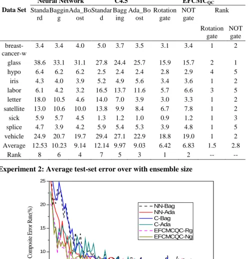
For the decision trees, the C4.5 and pruned trees are used which empirically produce better performance. We employed the Rotation gate and the NOT gate with the EFCMC_QC respectively. Results in Table 5 are the average error rate performed with ten cross validation folds by the Neural Network, C4.5 and EFCMC_QC respectively.

Experiment 1: Error Rates

Table 5 summarizes the average test error rates obtained when applying proposed EFCMC_QC in the the UCI data sets. It contains also the average test error rates of Bagging and Boosting ensembles with the neural networks and the C4.5 as the base classifiers for comparison. It can be noticed that our ensembles (EFCMC_QC), not only in the smallest data set labor (57 samples only) but the biggest data set

letter(as seen in Table 4, the number of samples is up to 20000), gives the most dominated superiority.

Table 5 Test set error rates

Data Set

Neural Network C4.5 EFCMC_QC

Standa rd

Baggin g

Ada_Bo ost

Standar d

Bagg ing

Ada_Bo ost

Rotation gate

NOT gate

Rank Rotation

gate NOT

gate breast-

cancer-w

3.4 3.4 4.0 5.0 3.7 3.5 3.1 3.4 1 2 glass 38.6 33.1 31.1 27.8 24.4 25.7 15.9 15.7 2 1

hypo 6.4 6.2 6.2 2.5 2.4 2.4 2.8 2.9 4 5

iris 4.3 4.0 3.9 5.2 4.9 5.6 3.4 3.6 1 2

labor 6.1 4.2 3.2 16.5 13.7 11.6 5.7 6.6 3 5 letter 18.0 10.5 4.6 14.0 7.0 3.9 3.0 3.3 1 2 satellite 13.0 10.6 10.0 13.8 9.9 8.4 6.7 7.8 1 2

sick 5.9 5.7 4.5 1.3 1.2 1.0 0.9 1.2 1 3

splice 4.7 3.9 4.2 5.9 5.4 5.3 3.9 4.8 1 5

vehicle 24.9 20.7 19.7 29.4 27.1 22.9 18.8 19.0 1 2 Average 12.53 10.23 9.14 12.14 9.97 9.03 6.42 6.83 1.5 2.8

Rank 8 6 4 7 5 3 1 2 -- --

Experiment 2: Average test-set error over with ensemble size

0 20 40 60 80 100

5 10 15 20 25

Composite Error Rate(%)

Number of Classifiers in Ensemble NN-Bag NN-Ada C-Bag C-Ada EFCMCQC-Rg EFCMCQC-Ng

Figure 1

Average test-set error over all 10 UCI data sets used in our studies for ensembles incorporating from one to 100 decision trees or neural networks.

Hansen and Salamon [42] had revealed that ensembles with as few as ten members are adequate to sufficiently reduce test-set error. Although it would be fitful for the earlier proposed ensembles, based on a few data sets with decision trees, Schapire [17] recently suggested that it is possible to further reduce test-set error even after ten members have been added to an ensemble. To this end, the proposed EFCMC_QC are applied with Bagging and Boosting ensembles to further investigate the performance variety relative to the size of an ensemble.

Figure 1 illustrates the composite error rate over all of ten UCI data sets for EFCMC_QC with Bagging and Boosting ensembles using up to 100 classifiers. The comparison results show that most of the methods produce similarly shaped curves. Figure 3 also provides numerous interesting insights. The first is that much of the reduction in error due to adding classifiers to an ensemble comes with the first few classifiers as expected. The second is that some variations exist in reality with respect to where the error reduction finally flattens. The last but the most important is that for both Bagging and Ada_Boosting applied to neural networks and the C4.5, much of the reduction in error appears to have occurred after approximately 40 classifiers, which is partly consistent with the conclusion of Breiman [14]. To our surprise, at 30 classifiers the error reduction for the proposed EFCMC_QC appears to have nearly asymptote to a plateau. Therefore, the results reported in this paper suggest that our method reaches convergence with the smallest ensemble size.

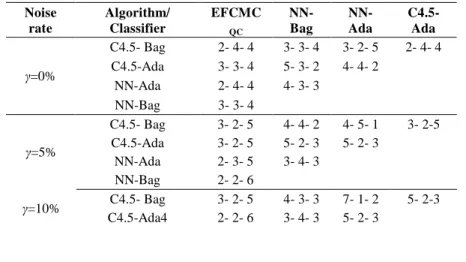
Experiment 3: Robustness of EFCMC_QC

To further test the EFCMC_QC performance, the different noise ratio is employed as Dietterich [43] in the four datasets satellite, sick, splice and vehicle. The four different noise ratios γ＝0%，γ＝5%，γ＝10% and γ＝15% are implied in the ten standard 10-fold cross validation, and results are described as follows:

Table 6

CV result on the satellite dataset Noise

rate

Algorithm/

Classifier

EFCMC

QC

NN- Bag

NN- Ada

C4.5- Ada

γ=0%

C4.5- Bag 2- 4- 4 3- 3- 4 3- 2- 5 2- 4- 4 C4.5-Ada 3- 3- 4 5- 3- 2 4- 4- 2

NN-Ada 2- 4- 4 4- 3- 3

NN-Bag 3- 3- 4

γ=5%

C4.5- Bag 3- 2- 5 4- 4- 2 4- 5- 1 3- 2-5 C4.5-Ada 3- 2- 5 5- 2- 3 5- 2- 3

NN-Ada 2- 3- 5 3- 4- 3

NN-Bag 2- 2- 6

γ=10% C4.5- Bag 3- 2- 5 4- 3- 3 7- 1- 2 5- 2-3 C4.5-Ada4 2- 2- 6 3- 4- 3 5- 2- 3

NN-Ada 2- 1- 7 2- 5- 3

NN-Bag 3- 2- 5

γ=15%

C4.5- Bag 3- 3- 4 4- 2- 4 7- 0-3 6- 2-3 C4.5-Ada 0- 3- 7 2- 4- 4 5- 3- 2

NN-Ada 0- 2- 8 2- 1- 7

NN-Bag 3- 3- 4

Table 7 CV result on the sick dataset Noise

rate

Algorithm/

Classifier

EFCMC

QC

NN- Bag

NN- Ada

C4.5- Ada

γ=0%

C4.5- Bag 3- 1- 6 5- 3- 2 5- 2- 3 3- 2-5 C4.5-Ada 4- 1- 5 6- 2- 2 6- 1- 3

NN-Ada 2- 1- 7 5- 1- 4

NN-Bag 2- 0- 8

γ=5%

C4.5- Bag 4- 1- 5 5- 3- 2 6- 2- 2 3- 4-3 C4.5-Ada 3- 1- 6 4- 4- 2 5- 2- 3

NN-Ada 2- 0- 8 4- 3- 4 NN-Bag 3- 1- 6

γ=10%

C4.5- Bag 4- 3- 3 4- 3- 3 7- 2- 1 5- 3-2 C4.5-Ada 2- 2- 6 3- 4- 3 5- 3- 2

NN-Ada 1- 1- 8 3- 3- 4 NN-Bag 3- 3- 4

γ=15%

C4.5- Bag 4- 3- 3 4- 2- 4 8- 1- 1 7- 1-2 C4.5-Ada 2- 1- 7 3- 2- 5 5- 2- 3

NN-Ada 0- 1- 9 6- 3- 1 NN-Bag 3- 6- 1

Table 8

CV result on the splice dataset Noise rate Algorithm/

Classifier

EFCMC

QC

NN- Bag

NN- Ada

C4.5- Ada

γ=0%

C4.5- Bag 2- 0- 8 3- 1- 6 3- 2- 5 4- 2- 4 C4.5-Ada 3- 1- 6 3- 1- 6 3- 4- 3

NN-Ada 3- 2- 5 4- 1- 5

NN-Bag 3- 3- 4

γ=5%

C4.5- Bag 3- 0- 7 3- 1- 6 4- 4- 2 5- 3-2 C4.5-Ada 3- 0- 7 3- 0- 7 2- 4- 4

NN-Ada 3- 3- 4 3- 3- 4

NN-Bag 3- 3- 4

γ=10%

C4.5- Bag 4- 1- 5 3- 3- 4 5- 3- 2 5- 4-1 C4.5-Ada 2- 0- 8 2- 1- 7 3- 3- 4

NN-Ada 3- 2- 5 3- 3- 4

NN-Bag 3- 3- 4 1 3 4 γ=15%

C4.5- Bag 4- 2- 4 3- 2- 5 3- 5- 2 5- 4-1 C4.5-Ada 1- 0- 9 0- 1- 9 2- 2- 6

NN-Ada 2- 2- 6 2- 3- 5

NN-Bag 4- 3- 3

Table 9

CV result on the vehicle dataset Noise

rate

Algorithm/

Classifier

EFCMC

QC

NN- Bag

NN- Ada

C4.5- Ada

γ=0%

C4.5- Bag 0- 0- 10 2- 1- 7 0- 2- 8 3- 1-6 C4.5-Ada 2- 0- 8 3- 1- 7 2- 2- 6

NN-Ada 3- 1- 6 4- 3- 3

NN-Bag 2- 1- 7

γ=5%

C4.5- Bag 2- 0- 8 2- 0- 8 3- 2- 5 4- 4-2 C4.5-Ada 2- 0- 8 1- 1- 8 2- 2- 6

NN-Ada 3- 0- 7 3- 4- 3

NN-Bag 4- 3- 3

γ=10%

C4.5- Bag 4- 0- 6 2- 3- 5 4- 5- 1 5- 4-1 C4.5-Ada 3- 0- 7 1- 0- 9 2- 2- 6

NN-Ada 3- 1- 6 3- 1- 6

NN-Bag 4- 3- 3

γ=15%

C4.5- Bag 4- 0- 6 3- 3- 4 4- 5- 1 6- 3-1 C4.5-Ada 2- 0- 8 1- 0- 9 3- 2- 5

NN-Ada 3- 0- 7 3- 1- 6

NN-Bag 4- 3- 3

From Table 6 to Table 9 it shows the average results of the ten-fold cross validation for the EFCMC_QC and other ensembles. Every number, e.g., 2-4-4 in the first place of Table 6, represents the times of performance results of the C4.5-Bag better than that of the EFCMC_QC is 2, equal to the EFCMC_QC is 4, and worse than the EFCMC_QC is 4.

These results also suggest that (a) all the ensembles can, at least to a certain extent, be inevitably affected by the noise. (b) the EFCMC_QC has more resistant not only to the ensembles with C4.5 but to the neural network, especially with greater noise ratio. The conclusion generally happened on the same dataset (e.g., satellite, sick, sick and vehicle) for all three ensemble methods. (3) for a problem with noise, focusing on misclassified examples would, to a great degree, cause a classifier tend to focus on boosting the margins of (noisy) examples that would in fact be misleading in overall classification which is obvious especially when the noise ratio becomes bigger. This phenomenon is consistent with the conclusion of David and Richard [44]. And (4) with the noise ratio becoming bigger, the

superiority of the EFCMC_QC in classification gradually becomes apparent. The bigger the noise ratio is, the more obvious its advantage is.

Conclusions and Future Directions

The paper has discussed relevant work, and proposed a novel ensemble strategy for the FCM classifiers, based on a novel evolutionary algorithm inspired by quantum computation for the FCMs. In this study, a comprehensive ensemble EFCMC_QC was then developed for the design of fuzzy cognitive maps classifier. It has been demonstrated how the EFCMC_QC helps construct classifier addressing the classification issue on a basis of numeric data. The feasibility and effectiveness of the EFCMC_QC were showed and quantified via series of numeric experiments with the UCI datasets. The follow-up results show that the proposed ensemble method is very effective and precede such traditional classifiers ensemble model such as the bagging and boosting. The future work will concern the use of the learning method in a context of more practical applications such as classification in dynamic systems and complex circumstances. Consummating the proposed EFCMC_QC and exploring applying area will be investigated.

Acknowledgment

This research is partially supported by the National Natural Science Foundation of China under grants 61300078 and 61175048.

References

[1] B. Kosko, “Fuzzy Cognitive Maps”, Journal of Man-Machine Studies, Vol.

24, No. 1, pp. 65-75, 1986

[2] D.-S. Chrysostomos and P.-G. Peter, “Modeling Complex Systems Using Fuzzy Cognitive Maps”, IEEE Transactions on Systems Man and Cybernetics- Part A Systems and Humans, Vol. 34, No. 1, pp. 155-166, 2004

[3] Z. Peng, B.-R. Yang, C.-M. Liu, “Research on One Fuzzy Cognitive Map Classifier”, Application Research of Computers, Vol. 26, No. 5, pp. 1757- 1759, 2009

[4] D.-Y. Zhu, B. S-. Mendis and T. Gedeon, “A Hybrid Fuzzy Approach for Human Eye Gaze Pattern Recognition”, In Proceedings of International Conference on Neural Information Processing of the Asia-Pacific Neural Network Assembly, Berlin, Germany, pp. 655-662, 2008

[5] A. Abdollah, R. Mohammad, B. Mosavi and F. Shahriar, “Classification of Intraductal Breast Lesions Based on the Fuzzy Cognitive Map”, Arabian Journal for Science and Engineering, Vol. 39, No. 5, pp. 3723-3732, 2014 [6] N. Ma, B.-R. Yang, Y. Zhai, G.-Y. Li and D.-Z. Zhang, “Classifier

Construction Based on the Fuzzy Cognitive Map”, Journal of University of Science and Technology Beijing, Vol. 34, No. 5, pp. 590-595, 2012

[7] J. Dickerson and B. Kosko, “Virtual Worlds as Fuzzy Cognitive Maps”, Presence, Vol. 3, No. 2, pp. 173-189, 1994

[8] A. Vazquez, “A Balanced Differential Learning Algorithm in Fuzzy Cognitive Maps”, In: Proceedings of the 16^th International Workshop on Qualitative Reasoning, Barcelona, Spain, pp. 10-12, 2002

[9] E. Papageorgiou, C.-D. Stylios and P.-P. Groumpos. “Fuzzy Cognitive Map Learning Based on Nonlinear Hebbian Rule”, In Australian Conference on Artificial Intelligence, Perth, Australia, pp. 256-268, 2003

[10] D.-E. Koulouriotis, I.-E. Diakoulakis and D.-M. Emiris, “Learning Fuzzy Cognitive Maps Using Evolution Strategies: a Novel Schema for Modeling and Simulating High-Level Behaviour”, In IEEE Congress on Evolutionary Computation (CEC2001), Seoul, Korea, pp, 364-371, 2001

[11] V.-C. Georgopoulos and C.-D. Stylios, “Diagnosis Support using Fuzzy Cognitive Maps combined with Genetic Algorithms”, 31^st Annual International Conference of the IEEE EMBS Minneapolis, Minnesota, USA, pp. 6226-2669, 2009

[12] Y. Engin and U. Leon, “Big Bang-Big Crunch Learning Method for Fuzzy Cognitive Maps”, International Scholarly and Scientific Research &

Innovation, Vol. 4, No. 11, pp. 693-702, 2010

[13] W. Stach, L. Kurgan, and W. Pedrycz, “Expert-based and Computational Methods for Developing Fuzzy Cognitive Maps”, Fuzzy Cognitive Maps, STUDFUZZ 247, pp. 23-41, 2010

[14] L. Breiman, “Bagging Predicators”, Machine Learning, Vol. 24, No. 2, pp.

123-140, 1996

[15] S. Hido and H. Kashima, “Roughly Balanced Bagging for Imbalanced Data”, In: 2008 SIAM International Conference on Data Mining, pp. 143- 152, 2008

[16] Y. Freund, “Boosting a Weak Learning Algorithm by Majority”, Information and Computation, Vol. 121, No. 2, pp. 256-285, 1995

[17] R. E. Schapire, Y. Freund, P. Bartlett and W. Lee, “Boosting the Margin: A New Explanation for the Effectiveness of Voting Methods”, In Proceedings of the Fourteenth International Conference on Machine Learning, Nashville, USA, 1997

[18] Y. Freund and R.-E. Schapire, “Experiments with a New Boosting Algorithm”, International Conference on Machine Learning, pp. 148-156, 1996

[19] E.-R. Schapire and Y. Singer, “Improved Boosting Algorithms Using Confidence-rated Predictions”, Machine Learning, Vol. 37, No. 3, pp. 297- 336, 1999

[20] D. Wolpert, “Staked Generalization”, Neural Networks, Vol. 5, No. 2, pp.

241-259, 1992

[21] S. Džeroski and B. Ženko, “Is Combining Classifiers with Stacking Better than Selecting the Best One?”, Machine Learning, Vol. 54, No. 3, pp. 255- 273, 2004

[22] P.-K. Chan and S.-J. Stolfo, “Toward Parallel and Distributed Learning by Metalearning”, In AAAI Workshop in Knowledge Discovery in Databases, Washinton D.C., USA, 1993

[23] P.-K. Chan and S.-J. Stolfo, “On the Accuracy of Meta-learning for Scalable Data Mining”, Intelligent Information Systems, Vol. 8, pp. 5-28, 1997

[24] S. Shilen, “Multiple Binary Tree Classifiers”, Pattern Recognition, Vol. 23, No. 7, pp. 757-763, 1990

[25] S. Shilen, “Nonparametric Classification Using Matched Binary Decision Trees”, Pattern Recognition Letters, Vol. 13, pp. 83-87, 1992

[26] P. Clark and R. Boswell, “Rule Induction with CN2: Some Recent Improvements”, Proceedings of the 5^th European Working Session on Learning, Springer-Verlag, pp. 151-163, 1989

[27] W. Leigh, R. Purvis and J.-M. Ragusa, “Forecasting the NYSE Composite Index with Technical Analysis, Pattern Recognizer, Neural Networks, and Genetic Algorithm: a Case Study in Romantic Decision Support”, Decision Support Systems, Vol. 32, No. 4, pp. 361-377, 2002

[28] A. -C. Tan, D. Gilbert and Y. Deville, “Multi-class Protein Fold Classification using a New Ensemble Machine Learning Approach”, Genome Informatics, Vol. 14, pp. 206-217, 2003

[29] P. Mangiameli, D. West and R. Rampal, “Model Selection for Medical Diagnosis Decision Support Systems”, Decision Support Systems, Vol. 36, No. 3, pp. 247-259, 2004

[30] O. Maimon, and L. Rokach, “Ensemble of Decision Trees for Mining Manufacturing Data Sets”, Machine Engineering, Vol. 4, No. 2, pp. 32-57, 2001

[31] L. Bruzzone, R. Cossu and G. Vernazza, “Detection of Land-Cover Transitions by Combining Multidate Classifiers”, Pattern Recognition Letters, Vol. 25, No. 13, pp. 1491-1500, 2004

[32] W. Chen, X. Liu, Y. Huang, Y. Jiang, Q. Zou and C. Lin, “Improved Method for Predicting Protein Fold Patterns with Ensemble Classifiers”, Genetics and Molecular Research, Vol. 11, No. 1, pp. 174-181, 2012 [33] F. Saima, A.-F. Muhammad and T. Huma, “An Ensemble-of-Classifiers

Based Approach for Early Diagnosis of Alzheimer’s Disease: Classification

Using Structural Features of Brain Images”, Computational and Mathematical Methods in Medicine Volume, Vol. 2014, 2014

[34] N. Sajid and K.-B. Dhruba, “Classification of Microarray Cancer Data Using Ensemble Approach”, Network Modeling Analysis in Health Informatics and Bioinformatics, Vol. 2, pp. 159-173, 2013

[35] P.-W. Shor, “Algorithms for Quantum Computation: Discrete Logarithms and Factoring”, In Proceedings 35^th Annu. Symp. Foundations Computer Science, Sante Fe, USA, pp. 124-134, 1994

[36] L.-K. Grover, “A Fast Quantum Mechanical Algorithm for Database Search”, In Proceedings 28^th ACM Symp, Theory Computing, Philadelphia PA, USA, 1996

[37] K. Han and J. Kim, “Quantum-Inspired Evolutionary Algorithm for a Class of Combinatorial Optimization”, IEEE Transactions on Evolutionary Computation, Vol. 6, No. 6, pp. 580-593, 2002

[38] Y. Kim, J.-H. Kim and K.-H. Han, “Quantum-inspired Multi Objective Evolutionary Algorithm for Multiobjective 0/1 Knapsack Problems”, In 2006 IEEE Congress on Evolutionary Computation,Vancouver, Canada, 9151-9156, 2006

[39] C. Blake, E. Keogh and C.-J. Merz, UCI Repository of Machine Learning Databases. Irvine: Department of Information and Computer Science,

University of California.

http://www.ics.uci.edu/~mlearn/MLRepository.html, 1998

[40] D. Rumelhart, G. Hinton and R. Williams, “Learning Internal Representations by Error Propagation”, In Rumelhart, D., & McClelland, J.

(Eds.), Parallel Distributed Processing: Explorations in the microstructure of cognition, Volume 1: Foundations Cambridge MA:MIT Press, pp. 318- 363, 1986

[41] J. Quinlan, “Introduction of Decision Trees”, Machine Learning, Vol. 1, No. 1, pp. 84-100, 1986

[42] L. Hansen and P. Salamon, “Neural Network Ensembles”, IEEE Transactions on Pattern Analysis and Machine Intelligence, Vol. 12, pp.

993-1001, 1990

[43] T.-G. Dietterich, “An Experimental Comparison of Three Methods for Constructing Ensembles of Decision Trees: Bagging, Boosting, and Randomization”, Machine Learning, Vol. 40, No. 2, pp. 139-157, 2000 [44] R.-L. Richard and P. -R. David, “Voting Correctly”, The American

Political Science Review, Vol. 91, No. 3, pp. 585-598, 1997

[45] K.-E. Parsopoulos, P. Groumpos and M.-N. Vrahatis, “A First Study of Fuzzy Cognitive Maps Learning Using Particle Swarm Optimization”, In

Proceedings of the IEEE 2003 Congress on Evolutionary Computation, Canberra, Australia, pp. 1440-1447, 2003