Quantum state identification of qutrits via a nonlinear protocol
P. V. Pyshkin1, A. G´abris2,1, O. K´alm´an1, I. Jex2 and T. Kiss1∗
1Institute for Solid State Physics and Optics, Wigner Research Centre, Hungarian Academy of Sciences P.O. Box 49, H-1525 Budapest, Hungary
2Czech Technical University in Prague, Faculty of Nuclear Sciences and Physical Engineering Bˇrehov´a 7, 115 19 Praha 1, Star´e Mˇesto, Czech Republic.
∗Corresponding author e-mail: kiss.tamas@wigner.mta.hu Abstract
We propose a probabilistic quantum protocol to realize a nonlinear transformation of qutrit states, which by iterative applications on ensembles can be used to distinguish two types of pure states. The protocol involves single-qutrit and two-qutrit unitary operations as well as post-selection according to the results obtained in intermediate measurements. We utilize the nonlinear transformation in an algorithm to identify a quantum state provided it belongs to an arbitrary known finite set. The algorithm is based on dividing the known set of states into two appropriately designed subsets which can be distinguished by the nonlinear protocol. In most cases this is accompanied by the application of some properly defined physical (unitary) operation on the unknown state. Then, by the application of the nonlinear protocol one can decide which of the two subsets the unknown state belongs to thus reducing the number of possible candidates. By iteratively continuing this procedure until a single possible candidate remains, one can identify the unknown state.
Keywords: quantum measurement, quantum control, quantum state identification.
1 Introduction
Measurement on a quantum system inevitably affects its state. One of the questions J´ozsef Janszky was intrigued by in his last active years was how one can design useful protocols involving post-selection based on measurement results [1, 2]. The power of measurement-based protocols can be used in quantum state purification [3–5], as well as for quantum state engineering [6–10], in particular also to cool down quantum systems to their ground-state [11–14]. One can exploit the nonlinear nature of this type of protocols for enhancing initially small differences between quantum states [15].
Discrimination of nonorthogonal quantum states is an important task for applications of quantum information and quantum control [16]. Various protocols have been proposed for efficient quantum state discrimination (QSD) (see reviews [17, 18]). A crucial ingredient of these methods is to have an ensemble of identical quantum systems for implementing QSD [19–22]. Measurement-induced nonlinear dynamics is experimentally feasible in quantum optics [23], and it has been shown [20, 22] that nonlinear quantum transformations could be a possible way for implementing QSD of two-level quantum systems. In this
arXiv:1808.10360v1 [quant-ph] 30 Aug 2018
are studied as candidates for quantum processing also experimentally, see e.g. [24].
Quantum state identification (QSI) is a problem where one has to decide whether an unknown quan- tum state is identical to one of some reference quantum states. In the original formulation of the problem [25, 26] the unknown pure state has to be identified with one of two or more reference pure states, some or all of which are unknown, but a certain number of copies of them are available [27, 28].
In this paper we design a quantum protocol based on post-selection where the difference between the absolute values of two coefficients in the expansion of the quantum state of a three-level system (qutrit) is enhanced. The protocol is thus capable of decreasing the overlap of initially nonothogonal ensembles of systems, according to a specific property of the states. We show that one can build an algorithm around this protocol which solves a quantum-state-identification type of problem where a finite number of reference states is classically given.
2 Nonlinear transformation of qutrit states
We consider an ensemble of identically prepared quantum systems in the state parametrized by two complex parameters,z1 and z2 as
|ψ0i=N
|0i+z1|1i+z2|2i
, (1)
withN = (1 +|z1|2+|z2|2)−1/2chosen such thatk |ψ0i k= 1. In the following we describe a protocol that allows us to distinguish between cases: (i) |z1|>|z2|and (ii)|z1|<|z2|, regarding the parametrization.
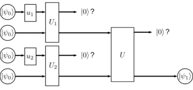
The core of this procedure is the nonlinear transformation schematically depicted on Fig. 1 as a quantum circuit diagram, with the single-qutrit unitary operators defined as
u1 =|0ih2|+|2ih0|+|1ih1|,
u2 =|0ih1|+|1ih0|+|2ih2|, (2)
and the two-qutrit operators as
U1 =|01ih11|+|11ih01|+ (1− |01ih01| − |11ih11|), U2 =|02ih22|+|22ih02|+ (1− |02ih02| − |22ih22|), U =|01ih10|+|10ih01|+ (1− |01ih01| − |10ih10|).
(3)
The procedure starts by taking two pairs of the system in initial state|ψ0i. Then one member of each pair is transformed by a single-qutrit unitary uj (j = 1,2), after which Uj acts on the pair of qubits as a whole, followed by perfoming selective projective measurementsP =|0ih0|on the first system of each pair. If both results are “yes” then we take the unmeasured systems from each pair and apply a joint unitary operatorU on them. Then we perfom again a projective measurement P on the first system in the pair, and if the result is again “yes” then the unmeasured system transforms into the state
|ψ1i=N0
|0i+z1 z2
z1|1i+z2 z1
z2|2i
. (4)
?
?
?
Figure 1: Scheme of the non-linear transformation|ψ0i → |ψ1ias a quantum circuit. Each line represents a qutrit.
By appling the above procedure to the entire ensemble of qutrits (always taking two pairs at a time) we arrive at a new albeit smaller ensemble constituted by identical states. We can interpret this as transforming an ensemble described by the state |ψ0i to an ensemble described by the state|ψ1i.
The transformation|ψ0i → |ψ1i is a nonlinear vector mapping:
f~(n)={f1(n), f2(n)}, f~(n)=f~(f~(n−1)), f~(0) ={z1, z2}, (5) where f1(n) = f1(n−1)2/f2(n−1) and f2(n) = f2(n−1)2/f1(n−1). Thus, the result of M iterations will be state |ψMi ∝ |0i+f1(M)|1i+f2(M)|2i. The map (5) has two attractors: {∞,0} and {0,∞}. There- fore, if |z1| 6= |z2| we will have for some relatively large M: |ψMi ≈ |1i in the case of |z1|> |z2|, and
|ψMi ≈ |2i in the case of |z1|<|z2|. We can distinguish these two cases, up to a certain error margin, by performing the projective measurement |1i h1| on the system in the state |ψMi, which allows us to draw conclusions regarding initial state|ψ0i. In Figs. 2(a) and 2(b) we show the probability of obtaining the state |1i in a measurement after one iteration (M = 1) and three iterations (M = 3) of the nonlin- ear transformation of Eq. (4), respectively. The border between regions with high and low probability corresponds to the|z1|=|z2|condition, and this border becomes sharper with increasingM. Thus, the reliablity of QSI increases with increasing M. Note, that the above discussed probability describes the precision of the discrimination process at the end of the protocol, yielding anerror marginon making the right conclusion about the given initial state [29]. Another relevant quantity is the survival probability which describes the post-selection process that is based on the intermediate projective measurements shown in Fig. 1. We will discuss this probability at the end of this Section.
The nonlinear transformation of Eq. (4) itself cannot distinguish two states in which|z1|=|z2|, as can be seen from Fig. 2. However, a properly chosen single-qutrit unitary operation can be used to make the magnitudes of these coefficients different so that the subsequent nonlinear transformation can distinguish such states. In order to show this, let us consider input states of the form
|ψ0i=N(|0i+ρ|1i+ρexp(iϕ)|2i), (6) whereρ, ϕ∈R. Then, apply the following single-qutrit unitary transformationR
R=
1 0 0
0 i/√
2 1/√ 2 0 −1/√
2 −i/√ 2
(7)
0 1 2 3
|z1|
0 1 2
|z2|
0 1 2 3
|z1|
0 1 2
|z2|
0.0 0.2 0.4 0.6 0.8
0.0 0.2 0.4 0.6 0.8
Figure 2: Probability of obtaining the state |1i in a measurement after M = 1 iteration (a) and M = 3 iterations (b) of the nonlinear transformation as a function of the parameters of the initial state given by Eq. (1). The thickness of the transient boundary is indicative of the error margin of correct identification.
on each initial state. Due to this operation the transformed state will be
R|ψ0i=N(|0i+z10 |1i+z20 |2i), (8)
where
|z01|=ρp
1 + sinϕ, |z20|=ρp
1−sinϕ. (9)
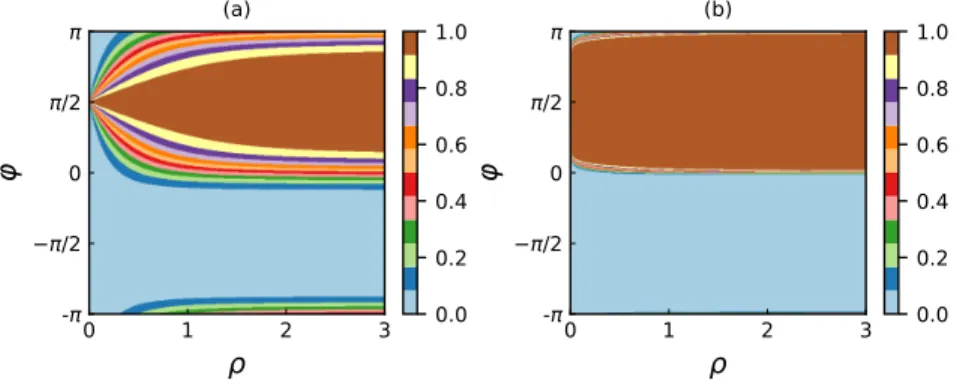
Therefore, we can treat the problem as before, since when ϕ 6= 0 then |z10| 6= |z02| and applying the nonlinear transformation on the state of Eq. (8) we can distinguish the two different situations: 0< ϕ < π (corresponding to |z01|>|z20|), and−π < ϕ <0 (corresponding to |z10|<|z20|). In Figs. 3(a) and 3(b) we show the probability of measuring state|1i as a function of the initial values ofρ and ϕ.
Figure 3: Probability of measuring state|1i after the application of the single-qutrit unitary operation of Eq. (7) and then the subsequent iteration (M = 1 for (a), and M = 3 for (b)) of the nonlinear transformation as a function of the parameters of the initial state of Eq. (6).
In practical situations the necessary number of iterations of the nonlinear protocol is determined by the probabilities depicted in Fig. 2 and 3. However, due to the fact that our nonlinear protocol is based on selective measurements, we need to have a relatively large number of identical qutrits in the initial
0.0 0.5 1.0 1.5 2.0
|z1| 0.0
0.5 1.0 1.5 2.0
|z2|
(a)
0.00 0.02 0.04 0.06 0.08 0.10
0.0 0.5 1.0 1.5 2.0
|z1| 0.0
0.5 1.0 1.5 2.0
|z2|
(b)
0.000 0.001 0.002 0.003 0.004 0.005
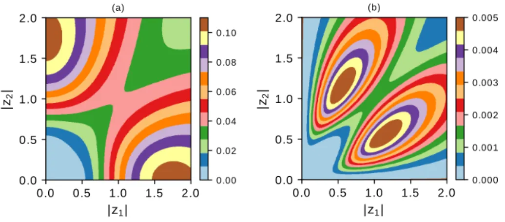
Figure 4: The overall survival probability of the nonlinear protocol forM = 1 (a), andM = 2 iterations (b) as a function of the initial parameters. Note that in the latter case the survival probability is given by the product of the Ps’s of the two steps. To determine the Ps of the second step, the transformed values ofz1 and z2 were substituted into Eq. (10).
state|ψ0i. This can be characterized by the survival probability in a single step Ps= |z1|2|z2|2+|z1|6+|z2|6
(1 +|z1|2+|z2|2)4 , (10)
which is the product of the three probabilities to measure |0i (see Fig. 1). From Eq. (10) it can be seen that the survival probability is very small (i.e., the protocol is very source demanding) when both z1, z2 → 0 or z1(2) → ∞. However, in cases when only a few iterational steps are expected to give a conclusive answer for discrimination, then the survival probability is also realtively high (see Fig. 4).
3 Quantum state identification of qutrits
Let us assume we have a “black box” that produces qutrits in the quantum state |ψ?i, which is unknown to us. What we know is that it belongs to a finite set S of possible qutrit states which we denote by
S=
|ψii=Ni |0i+zi1|1i+zi2|2i
|i= 1, . . . , K , (11)
with zij ∈ C being complex numbers. We also introduce the function N: S → N(S) denoting the number of elements in the set S, yielding N(S) = K in the particular case. The problem of quantum state identification (QSI) is to find w such that |ψ?i = |ψwi by applying quantum operations on the ensemble produced by the black box. For the sake of simplicity let us assume that |zi1| 6= |zi2| for all i∈(1,2, . . . , K). In case we have|zn1|=|zn2| for somenwe can apply a unitary rotation similar to the one in Eq. (7) to transform the coefficients into new ones of unequal magnitude.
Before discussing the QSI algorithm itself, let us consider the following unitary rotation:
W(θ) =
1 0 0
0 cosθ sinθ 0 −sinθ cosθ
. (12)
by the map in Eq. (5).
This can transform a quantum state of the form of Eq. (1) with|z1| 6=|z2|into the state with|z1|=|z2| ifθis chosen in the following way:
tan 2θ= |z2|2− |z1|2
z1z2∗+z∗1z2. (13)
Moreover, by choosing a different angle θ0 in such a way that θ < θ0 < π/4 (forθ >0) or −π/4< θ0< θ (for θ < 0) we can change the sign of |z1| − |z2|. We take advantage of such transformations in our quantum state identification algorithm, which is depicted in Fig. 5 by a flowchart.
The QSI algorithm of Fig. 5 is composed of calculational steps (with yellow background) in which the parameters of the necessary physical operations are determined and these are followed by the actual physical operations on the qutrit ensemble (with blue background). The description of the algorithm is
the following
Inputs: Set S as given by Eq. (11) with K ≥ 2 elements. Ensemble of qutrits in an unknown state
|ψ?i ∈S.
Output: Number wsuch that|ψwi=|ψ?i up to a desired error margin.
Procedure:
1. DivideS intoS+ (containing states with|zn1|>|zn2|) andS− (containing states with|zm1|<
|zm2|).
2. If both N(S+)>0 andN(S−)>0 then skip tostep 5, otherwise continue to the next step.
3. Determine a properθ with whichS can be divided into subsetsS+ and S− with N(S±)>0.
4. Apply the unitary rotationW(θ) of Eq. (12) to the ensemble with the unknown state|ψ?i.
5. Apply iteratively M times the nonlinear protocol of Fig. 1 to a sufficiently large ensemble representing the unknown state|ψ?i.
6. Make a projective measurement to decide whether the unknown state belongs to the set S+ or toS−, i.e. whether|zw1|>|zw2|or|zw1|<|zw2|should be satisfied by w.
7. If the result is “true” (i.e., in the projective measurement the state |1i was found) then we define S0 to be equal to S+, if the result is “false” (i.e., in the projective measurement the state|2i was found) then we set S0 toS−.
8. If the number of elements of the new setN(S0) = 1 then the single element of the set is equal to the unknown quantum (apart from possible W(θ) rotations), thus w has been found. If N(S0)>1 then repeat the whole procedure from step 1 withS set toS0.
0 1 2 3 4 5 6
Number of cycles
0.2 0.4 0.6 0.8 1.0
Pro ba bil ity of disc rim ina tio n
K=2 K=3 K=4 K=5 K=6
Figure 6: The average probability of correctly identifying the unknown quantum state among the given set (of sizeK) of qutrit states as a function of the number of iterationsM of the nonlinear transformation in step 5. No iterations yield the probability 1/K.
d=−D θ= (θbD/2c+θbD/2c+1)/2
−D < d≤ −2 θ= (θb−d/2c+θb−d/2c+1)/2
−1≤d≤1 θ= (θ1−π/4)/2
2≤d < D θ= (θbD−d/2c+θbD−d/2c+1)/2 d=D θ= (θbD/2c+θbD/2c+1)/2
Table 1: Optimized determination ofθ to divide S into S+ and S−. We have denoted the lower integer part of a real numberx by bxc.
The efficiency of our algorithm is illustrated in Fig. 6. We numerically simulated the QSI algorithm of Fig. 5 by choosing 20000 random realizations of sets of qutrit states of different sizes from K = 2 to K = 6. The coefficients zij = ρijexp(iϕij) of the states were given by choosing ρij and ϕij randomly from a uniform distribution in the interval [1/2,2) and [0,2π), respectively. The integer parameter w was randomly chosen in the range 1,2, . . . , K. As can be seen from Fig. 6 the results of our algorithm scale well with increasing set size. In fact, it is comparable to the well-known “weighing puzzle“, in which someone has to find a “false coin” in a given set of coins by using balanced scales [30]. In our numerical simulations if one of the subsetsS+ or S− was empty, then, for the states of the non-empty subset we calculated the ordered set θ1 < θ2 < · · · < θD by using Eq. (13) (where D is the size of non-empty subset). We counted the number n+ (n−) of positive (negative) θi’s and calculated their difference d= n+−n−. Then, we determined θ according to Table 1. Let us note that if θl =θm for some 1≤l, m≤K, then this procedure fails. As can be seen from Eq. (13) this occurs whenzmj =Azlj, wherej= 1,2, andA is some constant. In order to solve this problem we can apply theu2 single-qutrit unitary transformation of Eq. (2) in step 3 to every member of the set (11). Thus, if we initially have two states |ψli = Nl(|0i+zl1|1i+zl2|2i) and |ψmi = Nm(|0i+Azl1|1i +Azl2|2i), then after this transformation we will have |ψl0i=Nl0(|0i+z1
l1 |1i+ zzl2
l1 |2i) and |ψm0 i =Nm0 (|0i+Az1
l1 |1i+zzl2
l1|2i) and the correspondingθ angles will be different.
Due to the optimization we apply during every loop when dividing the set S, the average number of loops that are needed for the QSI algorithm to complete scales as lnK. In Table 2 we show the numerical results with the average number of loops and their standard deviations based on numerical simulations with 20000 random realizations of the set given by Eq. (11).
Set size K = 2 K = 3 K = 4 K = 5 K = 6
Average number of loops 1 1.89 2.58 3.16 3.66
Standard deviation 0 0.31 0.49 0.57 0.63
Table 2: Average number of loops of the QSI algorithm and their standard deviations for different set sizes.
4 Summary
We have presented a probabilistic scheme to realize a nonlinear transformation of qutrit states with two stable attracting fixed points. The nonlinear transformation is defined on an ensemble of quantum systems in identical quantum state, and in each elementary operation it uses two pairs of systems to probabilistically produce one system in the transformed state. Therefore, the protocol requires at least exponential resources in terms of the size of the ensemble as a function of the number of iterations.
The nonlinear map can be used to find out whether a given unknown pure state belongs to the subset converging to one of the attractive fixed points. We employed this property for QSI by proposing an algorithm that can be used to identify the quantum state from a finite setS of candidates, with an error margin. We have shown that the number of loops the algorithm uses scales logarithmically with the number of elementsK in the set S. While the error margin can be made arbitrarily small by increasing the number of iterationsM of the nonlinear map, the role and impact of the survival probability remains an open question that deserves further studies.
Our results indicate that probabilistic nonlinear schemes may offer a consistent approach towards QSI of higher dimensional systems, the present study on qutrits being the first step towards this direction.
Acknowledgments
The authors P. V. P., O. K. and T. K. were supported by the National Research, Development and Innovation Office (Project Nos. K115624, K124351, PD120975, 2017-1.2.1-NKP-2017-00001). In addition, O. K. by the J. Bolyai Research Scholarship, and the Lend¨ulet Program of the HAS (project No. LP2011- 016). I. J. and A. G. have been partially supported by MˇSMT RVO 68407700, the Czech Science Foundation (GA ˇCR) under project number 17-00844S, and by the project “Centre for Advanced Applied Sciences,” registry No. CZ.02.1.01/0.0/0.0/16 019/0000778, supported by the Operational Programme Research, Development and Education, co-financed by the European Structural and Investment Funds and the state budget of the Czech Republic.
References
[1] D. T. Pegg, L. S. Phillips, and S. M. Barnett,Phys. Rev. Lett. 81, 1604 (1998).
[2] M. Koniorczyk, Z. Kurucz, A. G´abris, and J. Janszky, Phys. Rev. A62, 013802 (2000).
[3] H. Nakazato, T. Takazawa, and K. Yuasa,Phys. Rev. Lett. 90, 060401 (2003).
[4] H. Aschauer, W. D¨ur, and H.-J. Briegel,Phys. Rev. A 71, 012319 (2005).
[5] J. Combes and K. Jacobs, Phys. Rev. Lett.96, 010504 (2006).
[6] P. J. Coles and M. Piani, Phys. Rev. A89, 010302 (2014).
[7] A. Streltsov, H. Kampermann, and D. Bruß,Phys. Rev. Lett.106, 160401 (2011).
[8] L.-A. Wu, D. A. Lidar, and S. Schneider,Phys. Rev. A 70, 032322 (2004).
[9] P. V. Pyshkin, E. Y. Sherman, D.-W. Luo, J. Q. You, et al., Phys. Rev. B 94, 134313 (2016).
[10] I. A. Luchnikov and S. N. Filippov,Phys. Rev. A 95, 022113 (2017).
[12] P. V. Pyshkin, D.-W. Luo, J. Q. You, and L.-A. Wu,Phys. Rev. A 93, 032120 (2016).
[13] J. B. Hertzberg, T. Rocheleau, T. Ndukum, M. Savva, et al., Nature Physics 6, 213 (2010).
[14] T. Rocheleau, T. Ndukum, C. Macklin, J. B. Hertzberg, et al.,Nature 463, 72 (2010).
[15] A. Gily´en, T. Kiss, and I. Jex, Sci. Rep.6, 20076 (2015).
[16] M. A. Nielsen and I. Chuang, Quantum Computation and Quantum Information (Cambridge Uni- versity Press, 2000).
[17] S. M. Barnett and S. Croke,Adv. Opt. Photon. 1, 238 (2009).
[18] J. Bae and L.-C. Kwek,Journal of Physics A: Mathematical and Theoretical 48, 083001 (2015).
[19] H. Mack, D. G. Fischer, and M. Freyberger,Phys. Rev. A 62, 042301 (2000).
[20] J. M. Torres, J. Z. Bern´ad, G. Alber, O. K´alm´an, et al.,Phys. Rev. A 95, 023828 (2017).
[21] W.-H. Zhang and G. Ren, Quantum Information Processing 17, 155 (2018).
[22] O. K´alm´an and T. Kiss, Phys. Rev. A97, 032125 (2018).
[23] J.-S. Xu, M.-H. Yung, X.-Y. Xu, S. Boixo, et al.,Nat Photon 8, 113 (2014).
[24] A. Abdumalikov Jr, M. Fink, J., K. Juliusson, M. Pechal, et al.,Nature 496, 482 (2013).
[25] A. Hayashi, M. Horibe, and T. Hashimoto,Phys. Rev. A72, 052306 (2005).
[26] A. Hayashi, M. Horibe, and T. Hashimoto,Phys. Rev. A73, 012328 (2006).
[27] U. Herzog and J. A. Bergou,Phys. Rev. A 78, 032320 (2008).
[28] U. Herzog,Phys. Rev. A 94, 062320 (2016).
[29] A. Hayashi, T. Hashimoto, and M. Horibe,Phys. Rev. A78, 012333 (2008).
[30] A. M. Chudnov,Discrete Math. Appl.25, 69 (2015).