Fault Detection in Dynamic Systems: From State Estimation to Direct Input Reconstruction Methods

From State Estimation to Direct Input Reconstruction Methods

F ROM S TATE E STIMATION TO D IRECT I NPUT

R ECONSTRUCTION M ETHODS

by

Dr. Andr´ as Edelmayer

Ph.D.

A DISSERTATION SUBMITTED IN PARTIAL FULFILLMENT OF THE REQUIREMENTS FOR THE DEGREE OF

D.Sc.

AT

HUNGARIANACADEMY OFSCIENCES

Budapest 2005

Computer and Automation Research Institute Hungarian Academy of Sciences

H-1111 Budapest, Kende u. 13-17.

Hungary

Fault Detection in Dynamic Systems:

From State Estimation to Direct Input Reconstruction Methods

1. Fault detection and isolation 2. Nonlinear systems 3. Dynamic inversion 4. Geometric system theory Typesetting in L^ATEX2ǫ: Camera ready by the author

°c Andr´as Edelmayer 2005 ALLRIGHTSRESERVED.

Give us time to work it out

For Moira Miranda Montealegre

Modern technology has increasingly created highly complex dynamical systems where the is- sues of systems’ availability and operational safety have become one of the main problems:

dependability and reliability became major concerns in the design of modern technical control systems. In engineering the term‘safety intensive’is used for denoting and characterizing these systems more closely. The scope of the theory and application of the technical and operational management of safety intensive systems is vast and increasing. This ranges from the most com- mon issues of operational safety such as condition monitoring, fault detection and isolation, fault diagnosis, fault management and fault tolerance to some more general questions of the operation such as the effect of human factor, mentioning just a few. Indeed, faults may have a considerable impact on the achievement of the system’s technical goal, on the security of human operators, on the integrity or on the profitability of the system itself, or on the integrity of the system’s environment. Practically, for safety intensive applications, every kind of system is concerned: embedded systems (for civil or military applications), or huge complex installa- tions, ranging from domestic systems to transportation, communication, industrial processes.

Their design must take into account safety and dependability considerations, for economic, sociologic and human reasons.

Incorporating safety issues into the design process is a rather contradictory problem, how- ever. Introducing dependability considerations into the design and the exploitation of systems has a visible cost, while the production losses, quality losses, performance degradations or even accidents which they would help to avoid are obviously not so apparent. In other words, sell- ing safety is not an easy problem in modern economy where the actors of the economy are mostly interested in maximizing their profits. In order to push decision makers of the economy towards the acceptance of safety regulations, and to encourage a volunteer approach to the consideration of those problems, it is necessary to develop techniques and application method- ologies which produce safe and secure systems at affordable prices, and in parallel, to develop analysis and evaluation tools in order to quantify, prove and certify the abovementioned sys- tems performances, that is to say, to increase the confidence measures of the application of the new safety intensive technologies.

Fault detection and isolation (FDI) issues, associated with fault tolerant control, have first been developed in the United States and in the former Soviet Union, mainly in the frame of defense and aerospace applications. Modern approaches of fault detection and isolation credited precursors from the early 70’s of a series of C. S. Draper Laboratory Studies at the

MIT, Massachusetts, USA, dealing with different aeronautic and navigation applications. Civil applications have been considered later, and mainly associated with huge programmes like nuclear power plants, chemical and petrochemical processes (following the occurrence of a number of technical disasters and industrial catastrophes). In this second period, European research laboratories have gained a very good expertise and have developed a real leadership in this area, because of the decrease of funding in the US, the political-economic crisis in Russia, and the recognition of the safety topic as a definitely important issue, which led to the funding of dedicated projects by the European Science Foundation (ESF), and of many projects and networks initiated by the European Commission (EC) within the international research programmesFP 4andFP 5. The research is now open for theFP 6framework initiatives whose individual projects were launched or were ready to be launched by 2004-2005, and, in April 2005, the EC published its proposals for the forthcoming FP7.

The increasing importance of the topic has been recognized by the creation of specific Tech- nical Committees (TC) by the International Federation of Automatic Control (IFAC), in addi- tion to existing committees in which the dependability considerations were already taken into account like the TC’s onSupervision in Chemical Industries, andComponents and Instruments.

The most specific TC, aimed atFault Detection, Supervision and Safety for Technical Processes, was created around the activity of the triennial symposia series SAFEPROCESS, which is now supported by approximately 50 members. It is meaningful to note that the first four SAFEPRO-

CESSconferences have been taken place in Europe, including the4^thmeeting, which was held in Budapest, Hungary, in the year 2000¹. SAFEPROCESS 2003 went outside of Europe and was held in Washington D.C., USA. These events summarized perhaps the best recent advances and activities in the area of safety intensive systems.

Another important milestone of the progress was thatsecurity and safety became closely coupled notions within automation and control: security, both in hardware and software tech- nology, has emerged as a high priority in many countries, especially after the shocking day of September 11, 2001, with its significant social and economic implications.

The major objective of the application of a fault detection methodology for dynamic sys- tems is to detect incipient faults and other disturbing patterns of the operation by isolating the failed system components in an attempt to prevent the development of (possibly global) malfunctions of the system liable to cause performance degradation and/or destruction of the equipment. Early detection of component malfunctions plays a fundamental role in advanced corporate management and in predictive maintenance planning.

The most common approach to FDI is the use of hardware redundancy, where measure- ments from multiple sensors are compared, and the existence of a failure is determined by implementing a voting mechanism. In many situations, however, hardware redundancy may not be possible or desirable, since it imposes a penalty in terms of volume, weight and cost, etc. In other situations, such as with actuators, the access to direct measurements is often not

1 The author is a member of the SAFEPROCESSTC. He was the chairman of the National Organizing Committee of SAFEPROCESS2000 and served as the editor of the proceedings volume of the conference featuring more than 200 technical contributions (Pergamon Press, London, ISBN 0 08 043250 6, Vols. 1/2/3).

possible and only indirect measurements may be used to infer the component fault status using an analytical model of the system. A possible method to analytically detect the existence of a failure is to look for anomalies in the plant’s output relative to a model-based estimate of that output by producing a residual signal that is zero in normal operation, but non-zero if a particular fault occurs.

Plant models, however, are generally incomplete and inaccurate, moreover, these fault de- tection and isolation algorithms often assume a particular failure mode. These plant dynamics and failure mode modeling errors can either cause a high false alarm rate, or make it difficult to detect faults. Any detection and isolation test that is designed to overcome the problems associated with these modeling errors has to be robust,i.e., it must be able to distinguish be- tween model uncertainties and failure modes and separate the effects of unmodeled dynamics or uncertain knowledge of the system parameters in order to avoid excessive false alarms or missed detections.

A possible approach to robust detection is based on the use of models, which describe the behavior of the plant more precisely. This often leads to varying structure, time dependent or nonlinear models the successful treatment of which depends on the development of new, more complex theories. The questions of robustness and sensitivity of the detection process, and the demand for new algorithms imposed by nonlinear problems are present implicitly in many approaches of the recent research. Robust FDI can be achievede.g., by assigning (decoupling) the fault effects and similarly the disturbances into disjoint subspaces in the detector output space, if possible. In many case, when this is not possible, approximate decoupling (in contrast to exact decoupling) is to be used. Approximate decoupling has to trade-off the amplification rate of fault effects and disturbances at the filter output. This problem usually leads to the theory of optimal filtering.

The author of this thesis volume has been involved in research and development of safety intensive systems for more than a decade. He took part in a number of industrial projects in the nuclear industry with activity of safety assessment, safety and reliability management, dependability analysis, dependable system installations and design. He is the author and co- author of a number of research papers in the field of fault detection and diagnosis.

The basic purpose of editing this volume together was to give a summary on the results accomplished by the author during the past ten years of research and characterize the achieve- ments which have been done in his post-doctorial work period. Another objective of this work is to enable the reader to follow the new developments in this area. It presents some fundamen- tals and advances of the theory and design of FDI methods, with special emphasis on the use of detection filters. The interested reader with no prior background in the problems of filtering and detection theory has many introductory textbooks to choose from. For a historical refer- ence the reader is directed to the succession of tutorials and survey papers in the constantly expanding literature.

In the past 15 years most of the work in FDI has been devoted to the generation of residuals in a framework referred to as analytical redundancy. While residual generation methods have been proposed in the literature in a great variety, two important tendencies of development

may clearly be recognized: a certain convergence of the approaches applied to linear systems and the attempt to the extension of linear results to nonlinear problems.

In this work we attempt to provide a brief summary on the general course of this devel- opment which lead researchers from the late 70’s to the most recent results of fault detection and isolation. In the framework of the theory of detection filters, we bring together two of the most exciting approaches of fault detection and diagnosis. The first involves residual genera- tion based on state estimation, the second is the subject of inversion-based direct input recon- struction: methods, both rooted in classical control and mathematical system theory that have considerable potential in a range of future applications. This treatment may well demonstrate the methodological convergence seen in linear approaches. We also provide the connection of ideas between the two areas demonstrating the progress from state estimation techniques to direct input reconstruction methods.

The discussion of the problems develops in two surfaces: the fields of linear and nonlinear problems. Though the unified treatment of linear and nonlinear approaches would be very for- tunate, the generalization of a linear approach to the nonlinear case cannot be done in every situation. While the solution of a robust estimation problem, for example, is crucial to solv- ing the robust fault detection problem effectively, traditional fault estimation techniques may not be applied to nonlinear problems with an ease. There are methods, however, originated in traditional state estimation techniques that provide extensibility of linear concepts to the nonlinear domain much easier: the system inversion based direct input reconstruction method not only demonstrates the existing analogies in between traditional linear approaches but also links together linear and nonlinear worlds in a straightforward way.

The presentation is organized as follows. In order to provide insight into the recent ideas one always need to look at the past, review the links between the main types of algorithms and have a view of their historical origins. Therefore, the historical outlook will be present in each of the chapters.

The thesis volume consists of four parts. The first part givingfoundations and outlookof the presented approaches familiarizes the reader with the basic definitions, properties and typical problems of fault detection and isolation. From the aforementioned reasons, in Chapter 1 a general system setup for modeling dynamical systems subject to faults and uncertainties is given. From the broad field of the theory of residual generation the parity space and the state estimation-based techniques are selected for comparison to review traditional (linear) residual generation methods. Special care is taken to provide a special view on the congruencies of these approaches.

The second part consists of three chapters. First, a geometric interpretation of the resid- ual is given in Chapter 2, which is supported by some background knowledge of geometrical system theory quoted from the literature. Chapter 3 reviews a range of optimization-based ap- proaches by using the standard problem formulation known from robust control, summarizing the role of state estimation approaches in robust fault detection and isolation. This chapter makes an effort to highlight distinctions as well as similarities between different well-known residual generation approaches, such as the Kalman filter, the optimalH_∞ filter and the vari- ous likelihood ratio tests. Though most of the detection approaches presented are based on a

deterministic setting, this chapter reviews a range of ideas regarding a stochastic setting giving different conditions of robustness when statistical properties of the disturbances are available.

As a direct response on the previous chapter, Chapter 4 continues with the discussion of op- timal game theoretic filters and illustrates the usefulness of these approaches to robust residual generation. It adds a little advance to the theory of traditional H_∞ detection filters by con- ditioning the optimization problem with scaling, all this in the framework of a deterministic problem formulation.

The third part deals with a completely new idea of residual generation which was given the title direct input reconstruction for fault detection. This part consists of three chapters again: first the original idea of the inversion-based input reconstruction method is introduced in an algebraic approximation in Chapter 5 for linear, and in Chapter 6 for nonlinear systems.

Chapter 7 highlights the same idea in view of a unified geometrical approach for both linear and nonlinear systems. In the course of the discussion, special attention is devoted to the con- cept how these methods could be extended from linear to nonlinear systems and under what conditions.

The parallelism between the linear and nonlinear approaches and the (sometimes hidden) interdependencies between the inversion-based and other traditional residual generation ap- proaches are always kept in front thus completing one of the basic objective of this work,i.e., to show the inherent congruences and interdependencies of the often sparsely interrelated ap- proaches. One of the most important such parallelism is revealed between the parity space and inversion-based detection approaches in Chapter 7.

To conclude the work and characterize the basic theoretical achievements given in this thesis, a case study is presented in Chapter 8 to demonstrate the effectiveness of the direct input reconstruction (inversion) method to fault detection and isolation. Quite unexpectedly, this case study serves not only for the purpose of an application example but it provides a framework of presentation upon which new results are built up. Based on various solution methods of the robust fault estimation problem represented by this real application example it is shown, how novel approaches to old problems may lead to new solution alternatives by demonstrating that advanced methods of filtering such as inversion-based residual generation andH_∞ optimal filtering and the novel combination of them may contribute to the solution of earlier not solvable problems: It is shown how the state estimate of the inverse dynamics could be obtainedon-lineby using conventional Luenberger-type state observers as well asH_∞ optimal filters, thus simplifying the filter design procedure, significantly.

We note that it was not(and itcould not) be possible to includeallthe most recent devel- opments in this area. Our story is only one of many, and other contributors all have at least as interesting, if not more interesting stories. New ideas in the field of fault detection and identification are not lacking, and we have suggested just a few during the last decade.

Budapest, September 2005 ANDR´_ASEDELMAYER

A

JOURNEY IS ALWAYS EASIER WHEN YOU TRAVEL TOGETHER.Interdependence is certainly more valuable than independence. This volume is the result of ten years work whereby the author has been accompanied and supported by many people. It is a pleasant aspect that he has now the opportunity to express his sincere gratitude for all of them. Systems and Control Laboratory (SCL) of Computer and Automation Research Institute of the Hungarian Academy of Sciences (MTA-SZTAKI) headed by Prof. J´ozsef Bokor was the first research site which, recognizing both theoretical and practical significance of fault detection and diagnosis, initiated research and development in this field in Hungary. In the course of the years, the laboratory has became one of the most acknowledged centers of excellence in the scientific world in this area.

It was the author’s pleasure to be able to join this activity at a very early stage and continue this work from the late 80’s belonging to the scientific community of the laboratory. Special thanks to MTA-SZTAKI which provided excellent conditions of research which helped to accomplish this work in the defined quality. The author is deeply indebted to Prof. J´ozsef Bokor whose help, stimulating suggestions and encouragement aided in all the time of the research. He was the first who put the idea forward and made the proposal for the realization of this project which ended with the preparation of this thesis volume. The author would like to express his sincere gratitude to Prof. Tibor V´amos and Prof. L´aszl´o Keviczky academicians and Prof. P´eter V´arlaki D.Sc. for their careful reading of the manuscript and for the many useful comments which allowed to improve the style of the presentation. He also expresses his gratitude to all members of SCL who substantially contributed to the development of this work. Special thanks to Dr. Zolt´an Szab´o and Dr. L´aszl´o N´adai for their fruitful discussions and valuable suggestions that considerably improved the content and presentation quality of this work. The author is grateful to Prof. Ferenc Szigeti for his unselfish help providing the sophisticated math background and rendering the sense and value of his unconditional friendship. It is also to be noted that the research has been supported by various grants and organizations. Special thanks to theHungarian Scientific Research Fund(OTKA) and theNational Research and Development Foundation(NKFP) which supported projects between 1996 and 2004.²

2”Analysis and Synthesis of Robust Detection Filter Design in Uncertain Dynamical Systems”, OTKA Grant No:

T 019448, 1996–1998,”Advanced Analytical Methods to Fault Detection and Isolation: Synthesis of Robustness and Sensitivity in Dependable Systems Applications”, OTKA Grant No:T 032408, 2000–2002,”COSMOS: Com- puterized operation support for the management, optimization and surveillance of large-scale industrial processes”, NKFP-2/016/2001, 2001–2004.

P

REFACE ₅

A

CKNOWLEDGMENTS ₁₁

P A R T 1

F OUNDATIONS AND O UTLOOK

1

M

ODEL

-B

ASED

D

ETECTION AND

I

SOLATION OF

F

AULTS IN

D

YNAMICAL

S

YSTEMS ₁₉

1.1 Introduction 20

1.2 Setup and problem formulation for linear systems 23

1.3 Nonlinear system models and their application in fault detection 26

1.3.1 Operation on vector fields 27

1.3.2 Symmetries, Poisson brackets and Hamiltonian representations 30 1.4 Residual generation for fault diagnosis in linear systems 32

1.5 The linear parity space approach 33

1.6 Observer-based residual generation in linear systems 35 1.7 On the equivalence relations of parity space methods and diagnostic observers

in linear systems 39

1.8 Summary 40

P A R T 2

R OBUST E STIMATION AND F AULT D ETECTION

2

G

EOMETRIC

C

ONCEPTS IN

R

ESIDUAL

G

ENERATION FOR

L

INEAR

S

YSTEMS ₄₃

2.1 Introduction 44

2.1.1 Elementary invariant subspaces 44

2.1.2 Self-contained controlled and conditioned invariants 45

2.2 Some specific computational algorithms 47

2.3 The concept of unknown input observer for linear systems 49

2.3.1 System invertibility and reconstructability 51 2.4 Geometric interpretation of the residual for linear systems 53 2.5 The fundamental problem of residual generation in linear systems 54

2.5.1 FPRG for two failure modes 54

2.5.2 Extension of FPRG to multiple faults and the relation to system invertibility 56 2.6 Detection and isolation by means of exact geometric decoupling in linear systems 57

2.7 Generalized state observer for LTV systems 59

2.7.1 Controllability and observability of LTV systems 60

2.7.2 Detectability of LTV systems 60

2.8 Summary 63

3

R

OBUST

E

STIMATION AND

F

AULT

D

ETECTION ₆₇

3.1 Introduction 68

3.2 System model, fault model 69

3.3 LRT with robustness to failure mode and noise model neglecting plant uncer-

tainties 73

3.4 LRT and plant modeling uncertainties 75

3.5 FDI with robustness to failure mode, noise and plant model uncertainties 77

3.5.1 The decision function 78

3.5.2 The robust estimator 80

3.6 Risk seeking estimation 81

3.7 Summary 82

4

G

AME

T

HEORETIC

R

OBUST

O

PTIMAL

E

STIMATION IN

L

INEAR

S

YSTEMS ₈₅

4.1 Introduction 85

4.2 Filtering in an H_∞ setting 88

4.2.1 The classical solution toH_∞ detection filters 88

4.2.2 Characterization of filtering sensitivities 90

4.3 ScaledH_∞ detection filters 91

4.3.1 Scaling and the idea of scaledH_∞ optimization 91 4.3.2 LMI solution of diagonally scaled optimization 92

4.3.3 Scaling and rotation of the worst-case input 94

4.4 Summary 96

P A R T 3

D IRECT I NPUT R ECONSTRUCTION

TO F AULT D ETECTION

5

I

NPUT

R

ECONSTRUCTION BY

S

YSTEM

I

NVERSION

:

AN

A

LGEBRAIC

A

PPROACH TO

L

INEAR

S

YSTEMS ₉₉

5.1 Introduction 100

5.2 Input (fault) observability of LTI systems 102

5.3 A constructive algorithm for inversion of linear systems 103

5.4 Summary 109

6

I

NVERSION

-B

ASED

I

NPUT

R

ECONSTRUCTION FOR

N

ONLINEAR

S

YSTEMS ₁₁₁

6.1 Introduction 111

6.2 Invertibility and the relative degree of linear systems 112

6.3 Relative degree of nonlinear systems 115

6.4 Algebraic construction of the inverse for nonlinear systems 117 6.4.1 A recursive algorithm for calculation of the inverse 119

6.4.2 Examples 120

6.4.3 Output selection scheme No.1 to Example 6.12 122

6.4.4 Output selection scheme No.2 to Example 6.12 123

6.5 Summary 123

7

A G

EOMETRIC

V

IEW OF

I

NVERSION

-B

ASED

D

ETECTION

F

ILTER

D

ESIGN ₁₂₅

7.1 Introduction 126

7.2 Zeros and zero dynamics 127

7.2.1 Zero dynamics of SISO linear systems 127

7.2.2 Zero dynamics of MIMO linear systems 129

7.3 Geometric theory of inversion-based input reconstruction in LTI systems 130 7.4 Geometric theory of inversion-based input reconstruction in nonlinear systems 137 7.4.1 Nonlinear analog of transmission zeros and zero dynamics 137 7.4.2 Nonlinear systems with vector relative degree 139

7.4.3 Feedback linearization and dynamic inversion 143

7.4.4 Extension to LPV systems 144

7.5 Relationship of parity space and system inversion-based residual generation in

linear systems 145

7.6 Summary 148

8

C

ASE

-

STUDY ₁₄₉

8.1 Introduction 149

8.2 The F16XL aircraft monitoring problem revisited 151

8.2.1 Disturbance attenuation withH_∞ filtering 155

8.2.2 Inversion based fault decoupling with disturbance attenuation 157 8.2.3 Detection and estimation by means of direct input reconstruction 160

8.3 Summary 165

P A R T 4

C ONCLUSIONS AND R EFERENCES

9

C

ONCLUSIONS ₁₇₁

9.1 From stand-alone methods to embedded applications 172

9.2 Known issues 176

R

EFERENCES ₁₇₇

L

IST OF

P

UBLICATIONS ₁₈₅

FOUNDATIONS AND OUTLOOK

With the ever increasing safety and security requirements of advanced techni- cal systems there has been significant research activity for the enhancement of safety and reliability and, as a closely related field, in fault detection and diagnosis in the past fifteen years. Most of the efforts have been devoted to methods relying on the idea of analytical redundancy and the generation of residuals based on the knowledge of the mathematical model of the system.

While residual generation methods have been proposed in the literature in great variety, two important tendencies of development may clearly be rec- ognized in the past years: a methodological convergence of the approaches applied to linear systems and the attempt to the extension of linear results to nonlinear problems (Gertler, 2002). In order to provide insight into the recent ideas one need to look at the past, review the links between the main types of algorithms and have a view of their historical origins. Therefore, as an introduction, the basic definitions, properties and typical problems of model- based fault detection and isolation is presented and a general system setup for modeling dynamical systems subject to faults and modeling uncertainties is given. Special emphasis is taken on parity relations and diagnostic observers.

This, from the one hand, may well demonstrate the methodological conver- gence could be seen in linear approaches and, from the other hand, provides the theoretical basis to further discussion.

M ODEL -B ASED D ETECTION AND

I SOLATION OF F AULTS IN D YNAMICAL

S YSTEMS

T

HE BASIC OBJECTIVE OF A FAULT DETECTION METHODOLOGY applied to dynamic sys- tems is to provide techniques for detection and isolation of failed components. The most obvi- ous method for automatic fault detection is the use of hardware redundancy, where measure- ments from multiple sensors are compared with each other and the existence of a failure is determined by implementing a voting mechanism. In many situations, however, the applica- tion of hardware redundancy may not be possible or desirable, since it imposes a penalty in terms of volume, weight and costs etc. In other situations, such as with actuators, direct access to certain variables is often not possible via physical measurements. In these cases, indirect measurements may be used to infer the component fault status using a mathematical model of the system. Most of the model-based methods rely on the idea of analytical redundancy in which, — in contrast to physical or hardware redundancy, — real physical measurements are completed with analytically computed redundant variables.

One method to analytically detect the existence of a failure is to look for anomalies in the plant’s output relative to a model-based estimate of that output. Analytical redundancy takes two basic forms such as direct and temporal redundancy. Direct redundancy exist among rela- tionship of instantaneous sensor measurements. Temporal redundancy is based on relationship of dissimilar sensor measurements provided at different times and relates sensor outputs and actuator inputs. For an extensive discussion of the idea see (Chow and Willsky, 1984). In the following discussions we only consider temporal redundancy relations in dynamical systems.

Plant models, however, are generally incomplete and inaccurate. Moreover, fault detection and isolation methods often assume a particular failure mode. The plant dynamics and failure mode modeling errors can either cause high false alarm rates, or make it difficult to detect the failures. Any detection and isolation test that is designed to overcome the problems associated with modeling errors must be able to distinguish between model uncertainties and failures in order to avoid excessive false alarms or missed detections. The robustness and sensitivity issue of fault detection is in the focus of the research, worldwide.

One possible approach to robustness relies on the use of models that describe the behavior of the plant more precisely. The use of nonlinear system models, however, may lead to diffi- culties in real life implementation. The underlying problem with these methods is that most of the established standard results of linear system theory must be relinquished, even though they comprise the basis of our understanding of dynamical systems. But, perhaps more impor- tantly, nonlinear problems are often not tractable from a computational point of view. The challenge is therefore not only in the development of efficient failure detection methods in theory, but also in ascertaining they are computationally efficient and robust with respect to model uncertainties, unavoidable system variations and nonlinearities.

The contents of this chapter is as follows. In the introduction we briefly review the system of principles developed by the discipline of fault detection and isolation in the last two decades.

We start with reviewing the different types of tasks and layers in the field of fault diagnosis and continue with a general system setup, including the basics of systems and fault modeling. The basic concepts of the modeling of nonlinear systems and the approaches used dealing with nonlinear systems is summarized.

Both direct and indirect approaches of the general concept of analytical redundancy is reviewed. The parity or consistency equations method is thedirectimplementation of the con- cept of analytical redundancy as it uses and manipulates the measurement variables directly.

The traditional methods used for the implementation of residual generators in anindirectway are usually based on the error dynamics of a state observer. These approaches are used in a number of situations differing in the assumptions on noise, disturbances, robustness properties and in the specific design methods. For comparison, see representations in the literature such as (Mangoubi, 1998; Mangoubi and Edelmayer, 2000) and (Gertler, 1997).

An interesting relationship between parity space and observer-based approaches which can be revealed through the close analysis of these approaches are shown as a conclusion of this introductory part of this thesis.

1.1. INTRODUCTION

The development of model based diagnostic systems is aimed at detecting incipient faults, and following permanently the state of the supervised process on the basis of some a priori information of the plant dynamics. This a priori information is captured in the form of a mathematical representation which is called model.

Technically, a fault diagnostic system typically consists of three basic parts: a residual gener- ator, a residual evaluation module, and a decision logic, see Fig 1.1. A usual residual generator takes the actuator commands and the measured outputs of the supervised system as inputs, and it returns a signal (or a set of signals) that is called residual. In the absence of faults in the supervised system, the nominal value of the residual is theoretically zero, after the transient due to initial conditions has vanished. However, it becomes significantly different from zero when a particular fault occurs.

Residual

generation Residual

evaluation

Decision logic

- - - -

plant meas- urements

residuals fault

signatures

fault hypotheses

Figure 1.1. Computational stages of fault detection and diagnosis

The residual evaluation module has to detect, using adequate tests, when a given residual is indeed distinguishably different from zero. Finally the decision logic analyzes the result of the evaluation of a set of residuals, and, from the pattern of triggered and non-triggered tests, it returns a decision as to which component is faulty in the supervised system. The determination of the defective component is called fault identification or fault isolation, hence the name fault detection and isolation (FDI). In this work, we mainly focus on the design problems relating to the first part of the detection process, i.e., residual generators.

The system of principles used by the discipline of fault detection and isolation has been well categorized in the survey paper by (Willsky, 1976). It has been pointed out that there exist three different types of tasks or layers in the area of fault diagnosis, such as (1) fault detection, (2) fault identification, and (3) fault signal estimation.Fault detection consists of designing a residual generator that produces a residual signal enabling one to make a binary decision as to whether a fault occurred or not.Fault identificationimposes a stronger requirement: when one or more faults occur, the residual signal must enable us not only to detect that there are faults occurring in the system, but it must also enable us to identify (isolate) which faults have occurred at which time. In certain cases providing information about the real magnitude of the fault signal is required: fault signal estimation is the determination of the extent of the failure. The latter is done by trying to reconstruct the fault signals. The three tasks have been considered in a large number of books and papers, see e.g., the textbooks of (Basseville and Nikiforov, 1993; Chen and Patton, 1998; Gertler, 1998), and the references therein.

There are several methods used for generating residuals. Classical approaches to fault de- tection place emphasis on the use of a more or less accurate model of a linear time invariant (LTI) system and the whole problem of modeling uncertainty and its impact on the detection process is usually ignored. Actually, the physical parameters of a real dynamical system are rarely stay invariant as the time varies. Parameter variations and internal fluctuations are in- herent dynamical phenomena of physical systems. Moreover, the systems are in contact with a complex, unpredictable environment causing them to change their behavior in time. They are subject to disturbances and our observation is always corrupted by some unpredictable mea- surement noise. Since most systems are inherently nonlinear by their nature, the use of linear models results in modeling uncertainties due to neglected high order terms in the Taylor series expansion of the nonlinear description of the plant.

To reflect our imprecise or partial knowledge of that unpredictable behavior it is desirable to think of it as inherently uncertain. As a result, it becomes practically impossible to detect any changes with unlimited sensitivity in the practice. Namely, the consequence of the uncer- tainties is that actual measurements will never match the estimated values and residuals will

thus be nonzero even when there are any deviations in the system. Such kind of parasitic resid- ual variations may cause non-desirable false alarms which may undermine the reliability and dependability of the detection system in the practice.

A fundamental requirement of FDI methods implemented in process environments is to accomplish performance objectives in the presence of modeling uncertainties and uncertain measurement data. The major concern is detection performance,i.e., the ability to detect and identify faults promptly with minimal delays and false alarms even in the presence of envi- ronmental disturbances, unavoidable variations of system parameters when the mathemati- cal model of the system is imperfectly known. It has been recognized early that feasibility of FDI methods requires satisfactory robustness with respect to the effects of model uncertainties whose impact on the detection process cannot be ignored.

Another class of problems where FDI designs might lead to false alarms or missed detection, are those that are subject to substantialunknownnonlinear dynamics. Even for a process with aknownnonlinearity, most FDI design methods lead to a situation with large probabilities of false alarms, simply due to the fact that they rely on linear methods and, hence, erroneously tend to detect the nonlinear effects as faults. Nonlinear FDI detectors has until the late 90’s only been considered in rather few papers in spite of the tremendous problems caused by nonlinear phenomena. Nonlinearities in connection with FDI has shortly been discussed in (Frank, 1990) and in (Patton and Chen, 1996). Lately, however, there has been increased interest in this issue, for a short summary see e.g. (Frank et al., 2000).

Ensuring robustness is one of the most exciting problems in research and development of FDI systems. The first reasonably effective results in this area – in parallel with the latest results of the new normative approaches of robust control theory – have only emerged quite lately. The earliest results concerning robustness, such as e.g., the robust diagnostic observer scheme with respect to structured LTI system perturbations appeared, see e.g., (Olin and Rizzoni, 1991).

Reference (Douglas and Speyer, 1996) studied robustness issues of the FDI problem in the framework of the original detection filter idea.

There have been a number of papers on the disturbance decoupled estimation problem, or, what amounts to the same thing, the unknown input observer scheme, see e.g., (Ding and Frank, 1991), moreover, the robust eigenstructure assignment approach of (Patton and Chen, 1991), all of which taking the stand of perfect disturbance decoupling in LTI systems. Although there is extensive research in the field, this area has a substantial potential for both academic research and engineering development. Yet, there is an important literature on identification methods for faults detection and isolation (Isermann, 1993; Isermann, 1984; Basseville and Nikiforov, 1993) that tackles specifically multiplicative type faults and has been used with success on several applications.

One possible route towards improving robustness, on the one hand, consists in using mod- els which describe the behaviour of the plant more precisely. This often leads to the area of varying structure, linear time dependent as well as bilinear and nonlinear uncertain systems whose successful treatment depends on the developments of new models and new theories for these models. On the other, the use of nonlinear system models may lead us to a dangerous area. The basic problem with these approaches is that we have to abandon most of the well

elaborated standard results of linear system theory which form the basis of our understanding on the behavior of dynamical systems. But, perhaps more importantly, nonlinear problems may generate models which are computationally untractable. Therefore the challenge is not only in the development of efficient failure detection methods performing well in the theory, but also in making these methods computable and robust with respect to modeling uncertainties, un- avoidable system variations and nonlinearities. Our purpose is, therefore, to study questions regarding the effects of nonlinearities from this point of view.

Perhaps needless to say, there is a personal bias in the approaches we discuss in the next chapters. First of all, we concentrate on the use of advanced algebraic methods and geometric concepts of linear and nonlinear system theory which, according to our view, may contribute in significant ways to the development of new results in this field as well as avoiding computa- tional difficulties.

1.2. SETUP AND PROBLEM FORMULATION FOR LINEAR SYSTEMS

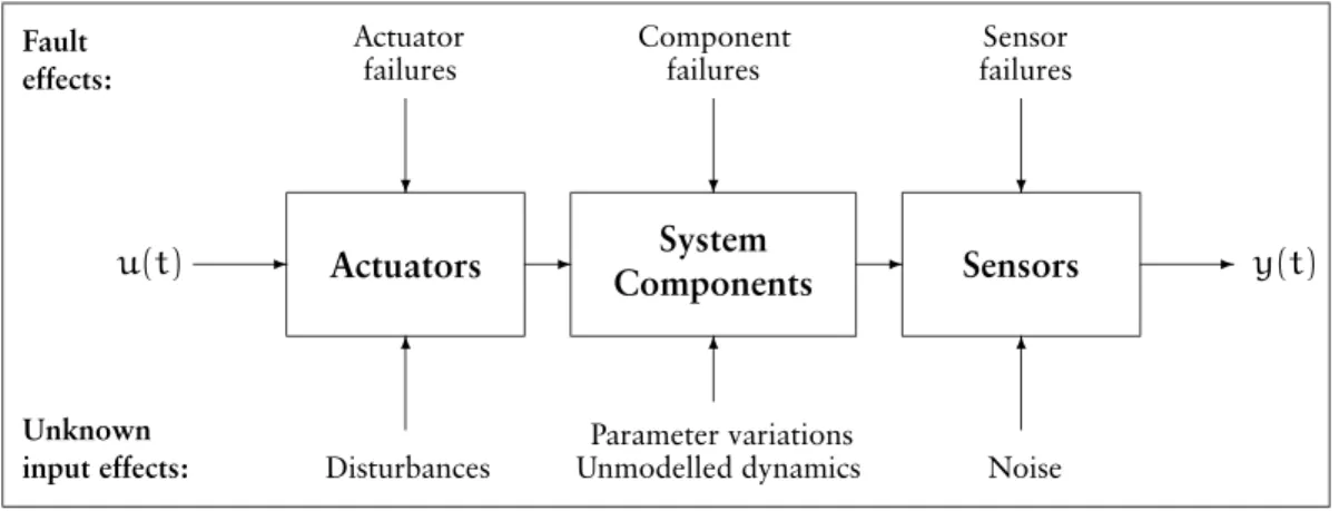
Consider the overall dynamical system as illustrated in Fig. 1.2 consisting of actuators, sensors and the main system components as usual. Actuators are driven by the input signalsu(t)while observation signalsy(t)are provided by the array of sensors. Malfunctions may occur either in the actuator and sensor dynamics as well as in the components of the system. The malfunctions can be treated separately and they enter the model as actuator, sensor or component failures.

Here we will consider methods developed for dynamic models in which the faults appear in the system as additive terms. This assumption is not very restrictive, as various type of faults, such as parameter changes or sensor failures, can be converted into additive type faults (with some non-negligible implications), for the proof of this proposition, see (Edelmayer, 1994). One of these possible implications is that even in time invariant systems, the coefficient of such faults is time varying, and another is that in case of handling a group of parameter changes this way,

Actuators System

Components Sensors

- - - -

6 6 6

? ? ?

u(t) y(t)

Unknown input effects:

Fault effects:

Disturbances

Parameter variations

Unmodelled dynamics Noise failures failures

failures

Sensor Component

Actuator

Figure 1.2. Characterization of the system in terms of faults and unknown inputs

it is possible to end up with ”equivalent” disturbances whose entry direction is colinear with most additive faults.

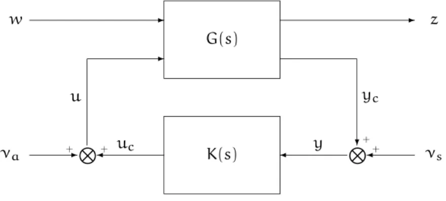
In normal conditions, the control literature means the termsystemwhich contains both the plant and the feedback controller at the same time (for a schematic representation see Fig 1.3).

Fault detection problems can be solved by using both closed-loop and open-loop methods.

Closed-loop methods consider the presence of the controller while open-loop methods are concerned with the problems without taking care of how the control signal is calculated.

We just note that if we work with a nominal system model in which modeling uncertainty and external disturbances are not considered, there is in principle no difference between open loop and closed loop detection methods. In the case of taking uncertainties into considera- tion, however, the good sensitivity performance of the fault detection method and the good performance of the closed loop control system operation is always compromised by each other.

Throughout the discussion of this paper we focus on open-loop detection and on modeling methods which does not incorporate the controller. It is always assumed that the state space description of the system is given by the nominal system matrices A, B, C, moreover, that the directions of the particular failures are known,i.e., the possible distribution (structure) of faults is known in advance from fault modeling. Obviously, inevitable modeling uncertainty arises due to external disturbances, sensor noise, internal system fluctuations, parameter variations and unmodeled system dynamics.

The uncertainty factors can be characterized asunknown inputsacting on the system. Their effect is described by perturbation techniques in the nominal system model. The choice of char- acterizing uncertainty depends highly on the purpose of modeling which may be varied from application to application. In fact, this is the factor what makes distinctive differences in the sequence of modeling approaches in this work. A general system setup, which can be applied

K(s) G(s)

-

N?+

¾ +¾ -

-

+ +N - ¾ w

y_c u

u_c y

νa

z

νs

Figure 1.3. Linear control system with actuator and sensor faults,νaandνs, respectively. G(s) is the system, K(s) is the controller.

in connection with fault detection and isolation for systems with model uncertainty, fault diag- nosis for systems with parametric system uncertainty and fault diagnosis for nonlinear systems is given in the following. This general setup is considered throughout the whole discussion of

this volume consistently, with obvious omissions and changes in the notations depending on the specialities of the problem to be solved.

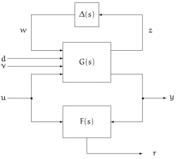
Consider the representation given in Figure 1.4, which is an extension of the setup shown in Figure 1.3, but without a feedback controller included.

∆(s)

F(s) G(s)

¾

--

-

¾

- -

-

-

• •

w z

u y

dν

r

Figure 1.4. General setup for robust fault detection in open loop.G(s)is the system,F(s)is the detector,∆(s)is the uncertainty description andris the residual.

The systemGin Figure 1.4 has the following state space realization:







˙ x z y





=







A Bw Bv Bd B

C_z D_zw D_zd D_zν D_zu Cy Dyw D_yd Dyν Dyu





















 x w d ν u

















, (1.1)

where x ∈ Rⁿ is the state vector, z ∈ R^q and y ∈ R^m are the external output signal and the measurement output signal, respectively. The maps A : X → X, B : U → X, are fixed throughout and will be associated with the nominal representation of the dynamical system described by the triple (A, B, C) (assuming D = 0 in the cases when generality is not lost).

Equivalently, the systemGcan also be given by its transfer functions à z

y

!

=

à G_zw G_zd G_zν G_zu G_yw G_yd G_yν G_yu

!











 w d ν u













. (1.2)

The inputs are external inputw ∈R^rfrom the uncertain block∆, disturbance inputd ∈ R^s, fault input signal ν ∈ R^k and the control input signal u ∈ R^p, respectively. Further, it is assumed that all other relevant weight matrices are included inG. The connection between the external outputzand the external inputwis given by the relationw=∆z.

The nominal system outputy(t)and inputu(t)are always assumed to be available through measurements and will be referred to as observables of the system. The vector valued function ν(t)is an arbitrary and unknown function of the time and is called failure mode of the system.

Note that by this definition of the failure mode we do not constrainν(t)to any special function class, therefore, a wide variety of faults can be modeled by this representation.

The general system setup given in (1.1) and (1.2) above describes a large class of differ- ent fault detection and isolation problems. The different cases will be characterized by the properties of the uncertainty block∆in Figure 1.4.

1.3. NONLINEAR SYSTEM MODELS AND THEIR APPLICATION IN FAULT DETECTION

In this work we are concerned with the continuous-time deterministic nonlinear systems de- scribed by ordinary differential equations

˙

x(t) = f(x(t), u(t)),

y(t) = h(x(t)) (1.3)

in which the control appears linearly (or affine) and which can be written in state space form, by means of a set of equations of the following type

˙

x=f(x) + Xm

i=1

g_i(x)u_i, (1.4)

y_i=h_i(x), 1≤i≤p,

wherex∈X⊂Rⁿ,u∈U⊂R^m,y∈R^pdenote respectively the state, the input and the output of the system. The mappings f, g1. . . , gmwhich characterize the dynamics of the system are Rⁿ-valued mappings defined on the open setX,i.e.,f(x), g₁(x), . . . , g_m(x) correspond to the values at a specific point x ∈ X in the state space. The functions h₁. . . , h_p are real-valued functions defined onX, andh₁(x), . . . , h_p(x)correspond to the values taken at a specific point xwhich characterize the output of the system. These mappings may be represented in the form ofn-dimensional vectors of real-valued functions of the real variablesx₁, . . . , x_n, as

f(x) =













f1(x₁, . . . , xn) f₂(x₁, . . . , xn)

... f_n(x₁, . . . , x_n)













, g_i(x) =













g1i(x₁, . . . , xn) g_2i(x₁, . . . , xn)

... g_ni(x₁, . . . , x_n)













, h_i(x) =h_i(x₁, . . . , x_n). (1.5)

System representation (1.4) can be extended with additional inputs which may represent faults and other unknown external excitations. One possible form of this extension can be written in

the form

˙

x(t) =f(x, u) + Xm

i=1

g_i(x, u)ν_i (1.6)

y_j(t) =h_j(x, u) + Xm

i=1

ℓ_ij(x, u)ν_ij, 1≤j≤p,

whereℓ_iare real valued functions defined onXandν(t)is the fault signal(ν₁, . . . , ν_m)^T whose elementsν_i: [0,+∞) →Rare arbitrary bounded functions of time inL₂. The fault signals ν_i can represent both actuator and sensor failures, in general.

The relationship of nonlinear system models (1.4) and (1.6) to linear systems can be estab- lished provided thatf(x), g_i(x), h_j(x), ℓ_i(x)are linear functions ofx,i.e.,f(x) =Ax,g_i(x) =b_i, h_j(x) = c_jx, ℓ_i(x) = d_ifor some n×n matrix A and b_i ∈ R^n×1, c_j ∈ R^1×n, d_i ∈ R^p×1, i= 1, . . . , n,j =1, . . . , p. This relationship between the classes of linear and nonlinear system models will be frequently referred to in the next sections.

The system representation (1.4) characterized above can be written in the form

˙

x(t) =A_ox(t) + Xk

i=1

a_i(t)A_ix(t) + Xm

i=1

u_i(t)B_ix(t), x(0) =x_o∈Rⁿ,

y(t) =Cx(t) (1.7)

assumingA_o, A_i∈R^n×nare linearly independent constant real matrices. We assumef:Rⁿ→ Rⁿ,g : Rⁿ→ R^m×n,h : Rⁿ→ R^p(and also a_i(t)) to be smooth (analytic) mappings. Note that the outputy(t) of the systems (1.4) and (1.7) which is affine in the inputs depends only on the statex(t).

The systems written either in the form of (1.4) or (1.7) describe a large number of physical systems of interest in many engineering applications, including fault detection and isolation. In respect of the application of different modeling formulations of systems of type (1.4) and (1.7) we shall be more specific later on.

1.3.1. Operation on vector fields

The mappings f, g₁. . . , g_m of the system models (1.4) and (1.6) are smooth mappings in their arguments assigning to each point x ∈ X a vector of Rⁿ, i.e., f(x), g₁(x), . . . , g_m(x), h₁(x), . . . , h_p(x) according to (1.5). Therefore they are referred to smooth vector fields de- fined onX.

DEFINITION 1.1. (Dual space of linear functional over X). The dual space X^′ of an n- dimensional vector space X can be identified with an n-dimensional vector space whose el- ements are called covectors. If {x₁, . . . , x_n} is a basis for X, the dual basis for X^′ is the set {x₁^′, . . . , x_n^′}⊂X^′ such thatx_i^′xj=δij(i, j∈n). ¤ LetS⊂X. The annihilator ofSdenoted byS^⊥ is the set of allx^′ ∈X^′ such thatx^′S=0. One can find thatS^⊥is a subspace of the dual spaceX^′.

Suppose now thatω1(x), . . . , ω_n(x) are smooth real-valued functions in the real variables (x₁, . . . , xn)ofX⊂Rⁿ, and consider the row vector

ω(x) =¡

ω1(x₁, . . . , xn). . . ωn(x₁, . . . , xn)¢ .

The mappingωassigning to each pointx∈Xan elementω(x)ofX^′ is called a covector field.

We will see that in many cases, it is more convenient to use, together with vector fields, the dual counterparts of these objectsi.e., covector fields assigning to each pointx∈Xan element of the dual spaceX^′.

A covector field that will be used more frequently in the following parts of this work is the socalleddifferentialof the real-valued functionλ. This covector field, denoteddλis defined as the 1×n row vector whose i-th element is the partial derivative of λwith respect to x_i. Its value at a pointxis therefore

dλ(x) =

·∂λ

∂x₁

∂λ

∂x₂· · · ∂λ

∂x_n

¸

, (1.8)

or simplydλ(x) =∂λ/∂x. Consider the real-valued functionλand a vector fieldfboth defined onX. A new function called the derivative ofλalongf, is the inner product, written as

L_fλ=hdλ(x), f(x)i= ∂λ

∂xf_i(x) = Xn

i=1

∂λ

∂xi

f_i(x). (1.9)

Repeated use of this operation lets extending the scope of the operation. The derivative ofλ first along the vector fieldfand then along a vector fieldgdefines

LgL_fλ(x) = ∂(L_fλ)

∂x g(x). (1.10)

Continuing a recursion by differentiatingλ k-times alongfsatisfies L^k_fλ(x) = ∂(L^k−1_f λ)

∂x f(x), with L⁰_fλ(x) =λ(x). (1.11) A standard assumption in modern control theory is that the state space (and the input and output space) are standard Euclidean vector spaces. This assumption is both valid and natural in many situations, but there is a significant class of problems for which it cannot be made. The Euclidean vector space is not a suitable state-space for a large class of nonlinear, time varying and varying structure control problems. Typical of these are the problems which arise in the control of systems type (1.7). The state space in this case is not a vector space.

It can be shown that the general description of nonlinear systems (1.4) and (1.7) which are considered throughout this paper can be properly defined on a state space which is not an Euclidean vector space Rⁿ, but instead is a curvedn-dimensional subset of R^m for some m which is called a manifold.

One of the basic problems with treating system models like representations (1.4-1.7) is that they usually do not describe the system everywhere, but only on a part of the state space.

For different part of the state space one may generally need another representation of the nonlinear system which can be obtained by mathematical transformations of (1.4) or (1.7). In geometrical language we say that Eqs. (1.4) and (1.7) are local coordinate descriptions of the

system. In order to cover the whole system behaviour, more than one coordinate description might be needed which require tedious mathematical calculations in the analysis.

There are approaches, however, which enable us to define a nonlinear system on a curved state space independently of any choice of local coordinates. It can be shown, for example, that an alternative (global) description of (1.4) and (1.7) evolves on a state space which in fact is a Lie group of the real orthogonal matricesA_i.

Application of the theory of Lie groups, Lie algebras and their representations is a rapidly growing field of modern mathematics which occure in the solution of problems in many fields of applied mathematics and physics. The related notions will be defined later in the next sec- tion.

Recent approaches of applied Lie theory are motivated basically by control theory. During the period from the early 60’s to the late 70’s, for example, several research papers appeared that made use of Lie algebraic techniques to study controllability of nonlinear differential equa- tions. These early results paved the way to a systematic use of these techniques in other system- theoretic studies.

There is another perhaps more important motivation behind the application of Lie theory to nonlinear problems. By embedding the original nonlinear problem in the framework of matrix Lie groups and associated Lie algebras, it is possible to reduce some system theoretic questions to problems which can be solved by using standard tools of linear algebra. Abstractly, a Lie algebraLrepresents a new kind of vector space to the problems which is equipped with a product [x, y], which is called Lie product or Lie bracket in the sequel, satisfying certain axioms.

In order to illustrate the idea consider, for instance, the varying structure and possible nonlinear system of (1.7) whereAo(x)andAi(x) are smooth vector fields defined in a neigh- borhood of the origin inRⁿ. Recall that a function defined in the Euclidean space Rⁿis said to be smooth at a point if it can be expressed as a convergent Taylor series in some neigh- borhood of that point. It can be shown that the local behavior of the system is determined by the algebraic properties of the iterated Lie products of the vector fieldsAo, A₁, . . . , A_k’si.e., the algebraic properties of the Lie algebra they generate. This is analogous to the fact that the local behavior of smooth functions is uniquely determined by its Taylor coefficients. Because of this fact, questions of dynamical properties of the above system can be reduced to symbolic questions about the algebraic properties of the non-commutative operatorsAo, A₁, . . . , A_k.

This is the problem of finding representations of the system in question invariant under a given Lie group of matrices. To be more specific, a challenging question is that of finding conditions under which, e.g., a linear time invariant (LTI) system is equivalent to one whose non-linear or linear time varying (LTV) dynamics is described by vector fields which generate a finite dimensional Lie algebra.

With the motivation of the use of Lie theory, a second type of operation on covector fields that is important to introduce here involves two vector fieldsfandg, both defined onX. From these a new vector field can be constructed, noted[f, g]and defined as

[f, g](x) = ∂g

∂xf(x) − ∂f

∂xg(x) (1.12)

at eachxofX, where the expressions

∂g

∂x =













∂g₁

∂x₁ · · · ∂g₁

∂xn

... ...

∂gn

∂x₁ · · · ∂gn

∂x_n













, ∂f

∂x =













∂f₁

∂x₁ · · · ∂f₁

∂xn

... ...

∂fn

∂x₁ · · · ∂fn

∂x_n













are the Jacobian matrices of the mappings g and f, respectively. The vector field defined in (1.12) is called the Lie product (or Lie bracket) of g and f. It is a fundamental property of Lie brackets that although they appear to be second order differential operators they are in fact first order because of the cancellation of the second order partial derivatives. To be more specific, the Lie bracket of two vector fields is always a vector field.

DEFINITION 1.2. (Lie algebra). A vector spaceV overRis a Lie algebra if in addition to its vector space structure it is possible to define a binary operationV×V → V, called a product and written[·,·], which has the properties

[v, w] = −[w, v] (1.13)

[α₁v₁+α₂v₂, w] =α₁[v₁, w] +α₂[v₂, w] (1.14) and satisfies the identity

[v,[w, z]] + [w,[z, v]] + [z,[v, w]] =0 (1.15) where α₁, α₂ are real numbers and v, w, zare real vector fields. Properties (1.13) and (1.14) are called the skew symmetric and bilinearity properties, respectively, and (1.15) is the Jacobi

identity. ¤

The importance of the notion of Lie bracket of vector fields and Lie algebras is very much related to their applications in the study of nonlinear systems of type (1.4) and (1.7). For demonstration, we give hereafter some interesting properties.

1.3.2. Symmetries, Poisson brackets and Hamiltonian representations

The Lie bracket operation (1.12) can be interpreted on linear maps and matrices. If, for exam- ple, we assume that

f(x) =Ax, g(x) =Bx then (1.12) reduces to

[f, g](x) = (BA−AB)x

where the matrix[A, B] = (BA−AB)is called the commutator ofA, B.

A matrix Lie algebra is an algebra of matrices with the commutatorXY−YX taken as the Lie bracket[X, Y]. One can immediately see that ifXandYare commutative matrices then their Lie product equals to zero. For example, from the skew-symmetric property[X, Y] = −[Y, X]it immediately follows that

[X, X] =0, and [X, Y] + [Y, X] =0.