Generalized persistent fault detection in distribution systems using network flow
theory
M´arton Greber∗Attila Fodor∗ Attila Magyar∗
∗Department of Electrical Engineering and Information Systems, Faculty of Information Technology, University of Pannonia, Egyetem
u. 10., Veszpr´em, H-8200, Hungary,
({greber.marton;fodor.attila;magyar.attila}@virt.uni-pannon.hu)
Abstract: Persistent faults are steady state anomalies with a magnitude which does not necessary trigger general protective gear. It is present in various types of distribution networks, as leak in pipe networks or as high-impedance fault in electric systems. As smart meters come into general use, distribution systems are upgraded to have advanced metering infrastructure.
The amount of consumer data is thereby increased, which can be used for diagnostic purposes.
Different kind of detection methods, improvements are presented in different physical domains.
However, persistent fault detection lies on basic physical principles like the conservation of energy. In order to be able to develop and evaluate methods, which target basically the same problems, the notions of the well established general network theory are being used. New formal definitions are presented to handle measurement data. In this framework a general extension of flow networks is presented which enables the detection of faults which are not present from the beginning in our model, between metered points. The solution to this problem is presented in the form of a two-stage evolutionary algorithm. Finally the working of the methods is illustrated and verified through a simple simulation based case study.
Keywords:Distribution networks; Smart power applications; Steady-state erors ; Losses;
Networks
1. INTRODUCTION
Distribution networks have the soul purpose to deliver re- sources from some supply entity to end consumers. Accord- ing to the type of the delivered resource, the networks take different appearances in the real world. Water and gas are transported through pipes, electricity is delivered through conductors. Effects from various sources like weather, ge- ographical location or human activity cause distribution lines to be vulnerable to faults. Persistent faults are steady state type faults. They can last relatively long because the magnitude of the faults is not big enough to trigger general protective gear.
Persistent faults can take many shapes according to the physical system. In electrical power distribution systems high impedance faults (HIF) can happen when at some point the distribution conductor is grounded through a high impedance, (Ghaderi et al. (2017)). Another example is the theft of electricity, also called non-technical losses (NTL). In this case live wires are manipulated to tap electricity or the measurement equipment is tampered, in order to hide consumption (Viegas et al. (2017)). Since more current needs to be supplied in order to keep existing demand satisfied, both cases lead to excessive load of the line and heat build up, in extreme case fire and blackout. In case of pipe network there are two main definitions called unaccounted for gas (UFG) and non- revenue water (NRW), both of these cover the same
topics, just in different technological context. In case of both, gas and water, resources are lost before reaching end customers. This is influenced by many factors like leakages, measurement variations and meter tampering, in case of gases there are also emissions . Real world case studies show, that leakage plays a considerable role both in UFG (Shafiq et al. (2018)) and NRW (Kanakoudis and Muhammetoglu (2013)).
Distribution systems nowadays are getting more and more support in terms of measurement equipment. Advanced metering infrastructure (AMI) relies on two way com- munication between the utility and the consumers (Jha et al. (2014)). This is enabled through smart meters, which are measurement devices capable of communication, to provide consumption data periodically. According to the type of distribution network, these are prominent in both electrical (Bahmanyar et al. (2016)), and water distribu- tion networks (Singapore (2016)). This data can also be used to perform various diagnostics on the network.
Since quality data is available, model based diagnostic methods present a powerful tool. As mentioned before, persistent faults are in general, leaks in distribution net- works. This phenomena has many sides, the detection can be split to many sub-problems.
In the case of NTL the general power balance equations need to be modified in order to account for wasted load.
Using the extended expressions it was noted that observing and comparing the voltage drop on line segments is an
indicator, and can be used for NTL detection (Bula et al.
(2016)). Since distribution networks can have large sizes, the question of structural decomposition and splitting a complex search into smaller units is an important task.
By incorporating parameter and measurement uncertainty into the model, the real world applicability of the devel- oped greatly increased (P´ozna et al. (2019)).
In case of water distribution networks, leakage detection can be formulated as an optimization problem where the difference between measured and estimated pressures is minimized. By incorporating a hydraulic simulator, leak- age scenarios are generated to locate leaks (Sousa et al.
(2015)). Until now, deficit was only assumed on metered points of the network. Another question is how to detect leaks between two metered points of the network, lying on a given pipe section. A steady state algorithm was devel- oped using pipeline dynamics, in order to test arbitrary points of a pipe section for leaks. This is achieved by a developed finite-difference approximation of the pipeline dynamics (Lizarraga-Raygoza et al. (2018)).
It can be seen that solutions for different aspects of the problem are already well established. However they are scattered in the different physical domains. On the other hand all of these distribution systems are governed by the same fundamental principles, for example the energy balance or the general Kirchoff’s laws. Flow networks are mathematical constructs involving graphs, and associating special properties to them (Iri (1969)). It is an already well established part of applied graph theory, capable of serving as a foundation to this task.
2. NETWORK FLOW
Graphs are mathematical constructs, which allow prob- lems to be translated into a structure consisting of ver- tices and edges. However in order to represent real world transportation networks in this context, the notion of graphs can be extended. By associating general attributes to vertices and edges, the resulting structure is called a flow network (Rockafellar (1998)).
2.1 General notions
In general a graph(G) is defined by three main compo- nents, vertices, edges and the connections between them:
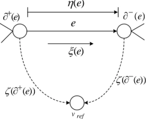
G= (V, E, ∂+, ∂−), (1) where V denotes the set of vertices V ={v1, v2, . . . , vm}, E represents the set of edgesE={e1, e2, . . . , en} and the connections are described as incidence relations:∂+:E→ V, ∂− : E → V. Throughout this work, directed graphs are used, which means that all the edges have directions.
A given edge e, is pointing from vertex ∂+(e) to vertex
∂−(e) (see Fig. 1.).
A flow network (N) consists of a graph, which is coupled with special attributes (Iri (1996)):
N = (G, ξ, η, ζ, f1, . . . , fn), (2) where ξ is the edge flow ξ : E → R, η defines the edge tension η : E → R and the relation between those two quantities is described by some branch characteristic function:ηi=fi(ξi) (see Fig. 1.). One vertex can be chosen as a reference point (vref) for measurements. This way we can associate potential values to vertices:ζ:V →R, which
represent the tension between some arbitrary vertex and the reference node. For a given edge, if one of the vertices isvref the branch characteristic description can be written as:ζi=fi(ξi).
)
(e
)
(e
)e
(e
(e)
)) ( (e
( (e))
vref
Fig. 1. Flow network notations
2.2 Distribution network flow
According to the function of a given edge, in distribution networks three main component categories can be distin- guished. Resources are being fed into the network through supply participants. These are transported through distri- bution line elements, to reach end consumer vertices. In order to give bounds to the topologies, the direction of these edges are fixed according to the rules below. Con- sumer edges point from arbitrary non-reference vertices to the reference vertex:
Ec={e|∂+(e)∈V \vref, ∂−(e) =vref}. (3) Supply edges point from the reference node to some arbitrary non-reference vertices:
Es={e|∂+(e) =vref, ∂−(e)∈V \vref}. (4) Distribution line edges point from some non-reference vertices to some arbitrary non-reference vertices:
El={e| ∂+(e)∈V \vref, ∂−(e)∈V \vref}. (5) The edge set for a distribution system flow network graph is defined as the union of the above mentioned sets:
E=Ec∪Es∪El. (6) Taking a distribution flow network, the general problem statement is the following, given
• Customer flow desires:ξ(e), ∀e∈Ec
• Supply at a given potential level: ζ(∂−(e)), ∀e∈Es
• Distribution system parameters:f1, . . . , fn
solve for:
• Changes in potential levels: ζ(v), ∀v∈V \vref
• Line flows:ξ(e), ∀e∈El.
For later use, the solution to this problem statement is described by the functionF.
F : (N, v)→R (7)
This takes a flow network N, solves the above described distribution network flow problem, and for a given vertex v it returns the calculatedζ(v) potential.
3. MEASURED FLOW NETWORK
The distribution flow network can be a projection of a real system. In order to incorporate measurement data for diagnostic purposes a similar but new concept is defined as measured flow network:
N˜ = (G,ξ,˜ ζ, f˜ 1, . . . , fn), (8) where ˜ζ is the measured potential ˜ζ : V → R and ˜ξ is the measured flow ˜ξ : E → R. This measured quantities represent different categories of real world measurement sources. Potential is measured at the non-reference vertices of consumers and supply points:
ζ(v), v˜ ∈ {∂+(e)|e∈ Ec} ∪ {∂−(e)|e∈Es} (9) Flow is measured on consumer and supply edges of the network:
ξ(e), e˜ ∈Ec∪Es (10) 4. PERSISTENT FAULT AT REGISTERED POINTS 4.1 Description
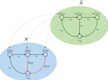
In case of fault situations regarding only registered points, the graph of the flow network and the graph of the measured flow network are identical. This means that the feeder and all the customers are measured points. If there is persistent fault, there is flow deficit, meaning that the registered amount of consumption is less than the supplied flow quantity.
) (v1
(v2) (v3)
vref 1
el el2
1 es
) (ec1
) (ec2
)
~( v1
~( )
v2
~( )
v3
vref 1
el el2
1 es
1 ec
2 ec
N~
N
Fig. 2. Example flow network compared to measured configuration
In Fig. 2. a simple flow network is depicted. There is one supply and two consumer elements. In case of a fault situation, the task is to determine the consumed flows to such an extent, that the potential values of the measured network flow structure are reproduced. The flow values in N are the variables which need to be determined (see red edges in Fig. 2.).
4.2 Detection
We have a flow network (N) and an associated measured network configuration ( ˜N). In order to verify the measure- ment data of ˜N, take the measured flows ˜ξ, plug them into
the flow network N, and solve the network flow problem.
This will provide the potential levels, according to the flow measurements. If the calculated potential values doesn’t match the measured potential levels:
∃v∈V \vref →ζ(v)6= ˜ζ(v), (11) the network has deficit. If the supplied amount of flow for a network doesn’t equals the consumed amount of flow, it is another indicator of a faulty network:
X{ξ(e)˜ |e∈Es} 6=X
{ξ(e)˜ |e∈Ec}. (12) In order to determine the valid consumer flow values the problem can be formulated as follows: minimize the differ- ence between measured and calculated potential levels, by adjusting the flow network’s customer flowsξEc.
arg min
ξEc
1 2
X
F(N(ξEc), v)−ζ(v)˜ 2
|,∀v∈V
(13) 5. PERSISTENT FAULT AT NON-METERED
POINTS 5.1 Description
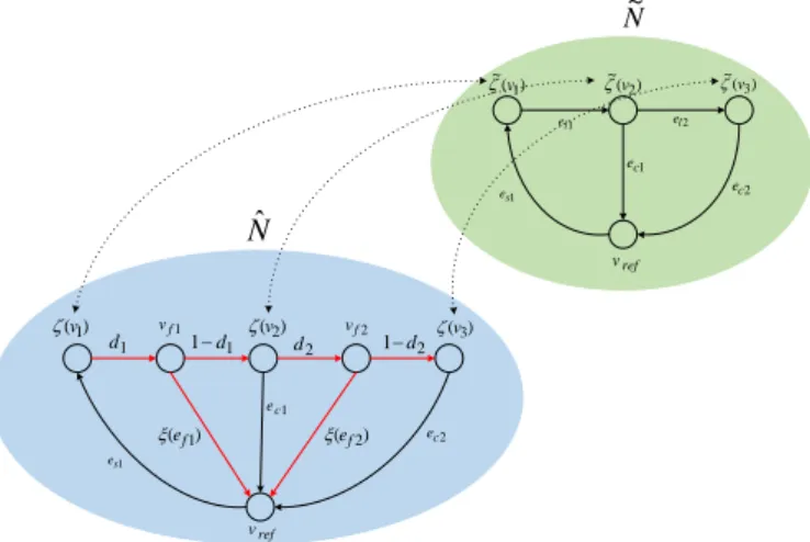
Faults can happen between metered points, which are new faulty nodes and are not present in the previous configuration. The goal is still the same, reproducing the potential measurement values from ˜N, by adjusting the consumer flow values in N. In order to represent these possible fault locations, the graph of N needs to be extended. The inserted node and edge properties are the unknowns, which must be adjusted to reproduce ˜ζ.
ej
vi vi1
vref fj
ej
vi vi1
vref dfj vf (1d)fj
ej
ef ) (ef
Fig. 3. Diagnostic node insertion 5.2 Detection
In order to be able to formulate the fault detection prob- lem, the creation of the extended network definition is nec- essary. For everye∈El line element, a new hypothetical fault node is inserted, by cutting in half the given edge. To represent the distance of the fault, from adjacent nodes the dividing pointd∈ {x|0 < x <1} is introduced. Spatial relation from the two nodes is represented by dividing the branch characteristic using d. The faulty flow values are modelled as a new vertex between the fault nodevf and vref, having ξ(ef) flow rate.
The diagnostic model needs are extended, in order to be able to calculate with non-metered points. Therefore all the distribution line elements must be changed, resulting in a set of new parameters. LetVf denote the vertex set of all the inserted fault nodesVf ={vf1, vf2, . . . , vf k},Ef
the appropriate fault flow edgesEf ={ef1, ef2, . . . , ef k}.
Existing line elements are cut into two pieces, for every
el∈El, two vertices are createde0l, e00l. The extended line segment set ˆEl is defined as:
Eˆl={e01, e001, e02, e002, . . . , e0n, e00n}. (14) From a flow network perspective the fault flow edges inEf
can be treated as consumer edges. The extended consumer edge set ˆEc, is the union of Ec and the fault edges:
Eˆc = Ec ∪Ef. In order to extend an existing G graph, the following steps can be used:
(1) given an existinge∈El line element with∂+(e) and
∂−(e) end nodes
(2) do the cutting, e will become e0 and e00, and insert the hypothetical fault nodevf:
• ∂+(e0) =∂+(e) and∂−(e0) =vf
• ∂+(e00) =vf and∂−(e00) =∂−(e)
(3) insert the edge ef representing the deficit flow:
∂+(ef) =vf and∂−(ef) =vref
Using this preliminary statements the extended diagnostic graph can be defined:
Gˆ = ( ˆV ,E, ∂ˆ +, ∂−), (15) where ˆV is the extended vertex set ˆV =V ∪Vf and ˆE is the extended edge set ˆE=Es∪Eˆc∪Eˆl.
Using this extended graph notation, the extension for the network flow can be constructed:
Nˆ = ( ˆG,ξ,ˆζ, D, fˆ 1, . . . , fn), (16) whereDis the set of division points,D={d1, d2, . . . , dk}.
Flow network calculation on the extended network is defined in the same way as it was defined before for a generalN.
) (v1
(v2) (v3)
vref 1 vf
1 es
1 ec
2 ec
)
~( v1
~( )
v2
~( )
v3
vref 1
el el2
1 es
1 ec
2 ec
N~
Nˆ
2 vf
) (ef1
(ef2)
d1 1d1 d2 1d2
Fig. 4. Extended network compared to measured flow configuration
The optimization problem which lies under this fault de- tection task is similar to the registered point case. How- ever now the graphs of the calculated and the measured networks are different. The values of the division points and the theft flows needs to be adjusted in such a way that on the metered pointsv ∈V the difference between measured and calculated potential values is minimized.
By denoting the set of flows associated to fault edges by ξˆEf ={ξ(e)ˆ | e∈ Ef}, the optimization problem can be formulated as follows:
arg min
ξˆEf,D
1 2
X
F( ˆN( ˆξEf, D), v)−ζ(v)˜ 2
| ,∀v∈V
s.t.: X
{ξ(e)ˆ | e∈Es}=X
{ξ(e)ˆ | e∈Eˆc} (17) 5.3 Genetic algorithm
Throughout network flow calculations the solution method consists of using Kirchoff’s laws and the branch character- istics. As stated before, consumption flows are an input parameters for the network flow, these are incorporated in the Kirchoff’s laws. The second components are branch characteristics, for obtaining the results in potentials.
In the optimization formulation above, both the branch characteristics, and part of the network consumptions are variables. Therefore the problem is of non-linear nature, with high number of unknowns. However the structure of the problem offers some opportunities to tailor the optimization method for this specific problem.
Genetic algorithms (GA) are optimization procedures in- spired by the evolution theory of Darwin. For a given problem some solution candidates are generated, and the goodness of them is evaluated. This is a generation, and members are transferred into an upcoming generation ac- cording to some rules (Sivanandam and Deepa (2008)):
• elitism: some percent of the top ranked members are automatically transferred,
• recombination: new solutions are created by combin- ing the properties of existing candidates,
• mutation: the solutions are tweaked in a random fashion .
In the new generation the goodness is evaluated again, the the procedure continues until some threshold value is reached or the maximum generation limit is exceeded.
Genetic algorithms offer a robust method even for hard op- timization problems, since the solution algorithm is almost the same in every case. However as with all soft computing techniques it doesn’t necessary give exact optima, most of the time close to optimal solutions are reached.
In case of evolutionary optimization the two main tasks are to determine the solution(chromosome) representation, and the measure of goodness, the fitness function. By distributing the contents of the unknown sets into one vector a simple chromosome representation is obtained:
pi= [ξ(e1), d1, ξ(e2), d2, . . . , ξ(ek), dk]. (18) As the measure of the fitness the optimization expression of equation 17. is used.
5.4 Two-stage evolutionary optimization
As mentioned before, the fault detection optimization problem is highly non-linear and since all the distribution edges are cut into half, the search space is enormous.
Therefore a single run genetic algorithm would require a high population size, with a high number of generations.
Experimental runs showed that it is still not enough to pinpoint a fault location. What the results showed, so called hot-spots of the fault were identified. Meaning that fault flows were inserted in some neighbourhood of the actual fault location. The idea is to run two consequent
optimization runs, where the first is to approximate the fault hot-spots, and the second to pinpoint accurate lo- cation and flow values. The effect of this two-stage GA is the implicit restriction of the search space during the whole process.
In the first stage the initial population P = [p1, p2, . . .]
is created in a totally random manner. Meaning that the entries of each pi are randomized, but in such a way that the constraint of equation 17. is taken into account. By taking the supply flows, and subtracting the metered consumption, the amount of deficit flow can be determined:
ξ∆=X
{ξ(e)˜ |e∈Es} −X
{ξ(e)˜ |e∈Ec}. (19) The only thing to take care is that the sum of the fault flow values in a given chromosome are equal to ξ∆. After executing the GA, using the incidence relations and the best member of the final population the number of hot- spots, and the cumulative fault flow in that region can be determined. We omit accurate location approximation and fault flow detection, by using a lower population and generation count, but the process is accelerated.
In the second stage, the initial population is generated using the hot-spot informations from the first run. Let us have hnumber of regions of interest, and the local cumu- lative fault flows are denoted by ξiH, i∈ {1, . . . , h}. The initialization is done, by assigning random flow indexes to eachξHi in each chromosome. In this step the search space is heavily reduced in the flow dimensions, by using the cumulative flow values the real task is to determine the correct set of division points.
6. CASE STUDY
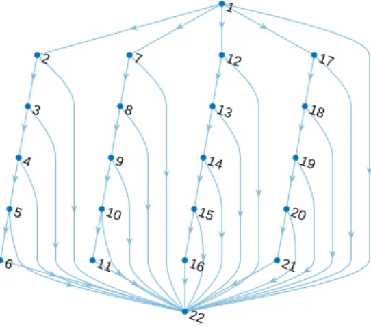
A simple case study example is created in order to il- lustrate the methodology. The topology of the network is presented in Fig. 5. This is an electrical network with radial layout. The feeder is at node 1, the reference vertex isv22.
1
2
3
4
5
6
7
8
9
10
11
12
13
14
15
16
17
18
19
20
21
22
Fig. 5. Case study network
The feeder point is modelled as a constant voltage source, consumer edges are constant current sources and con- nection line elements are resistive components. This is a homogeneous test case, meaning that all the line elements and all the consumer elements are of equal value. The line
elements have a resistance of 0.1Ω and all the consumers are 1A. The feeder point supplies the network as a 230V voltage source.
In order to use the methodology presented in the previous sections, the electrical network must be translated into that framework. Network currents are equal to edge flows:
I ξ, and electrical potential is equal to network flow potential: φ ζ. The translated distribution system properties are:
• Customer flow desires:ξ(e) = 1, ∀e∈Ec.
• Supply at a given potential level: ζ(∂−(e)) = 230, ∀e∈Es.
• Distribution system line parameters:ηi= 0.1ξi Resistive networks are basic electrical systems, which are covered by Ohm’s law:
U =RI, (20)
whereU is voltage,R is resistance andI is current. This is a linear network, by using node quantities the flow problem can be written asφ=RI, whereφ∈Rmis the potential vector,R∈Rm×mis the nodal resistance matrix and I ∈ Rm is the nodal current injection vector. The network flow calculation F is thereby a linear problem.
The following simulations were performed using MATLAB where the methodology was implemented.
6.1 Fault at registered point
Let us suppose that we have the above introduced test case, and persistent faults are only allowed at registered points. In order to generate measurement data, a sim- ulation was run ( ˜N), where the consumption connected to nodes 9 and 20 is changed from 1 to 2 and 3.5. The resulting potential values are stored for ˜ζ. The task is to find the faulty nodes, utilizing the measurement potential values.
Fig. 6. Potential values
We run the network flow calculations and plot every potential value (Fig. 6. blue line). Next we observe the available measurement data, which is visualized with red in Fig. 6. It can be seen that there is a substantial difference between them. This satisfies the deficit criteria state in equation 11. The faults can be detected using linear least- squares formulation, since the network flow calculation of the underlying DC network is a linear problem. The inbuilt function lsqlin() in MATLAB was used in order to solve this problem, since it can solve tasks in the form of:
minx
1
2||Cx−d||22, (21) whereCxrepresents the linear flow calculation anddthe measured quantity. Running the optimization function,
and plotting the results, the faulty nodes can be observed, alongside with the respective fault flows(see Fig. 7.)
1
2
3
4
5
6
7
8
9
10
11
12
13
14
15
16
17
18
19
20
21
22
2.0000 3.4999
Fig. 7. The network with the detected fault nodes 6.2 Fault at non-metered points
Two faults are inserted also in this test case. However, now they are inserted between two existing vertices. One fault was inserted between nodes 9 and 10, with a dividing point of 0.331 and a fault flow of 3.3. The second fault lies between nodes 20 and 21, with a dividing point of 0.218 and a fault flow of 1.7. in order to generate measurement data, these faulty points are inserted into the graph.
Potential measurements are taken from vertices 2, . . . ,21, and stored in a measurement flow network ˜N. Using the nominal consumption the expected potential profile is calculated by solving the linear network flow problem. The two sets are compared, and since there is a difference, one can begin with the detection algorithm.
Fig. 8. Potential values
The solution is reached using the two-stage evolutionary algorithm. In both stages a population size of 5000, a maximum generation number of 50 is used. The rate of elite selection is 20%, whereas the mutation is set to 2%. For reproduction, single-point crossover is utilized. In order to ensure the optimization constraint of equation 17. a penalty function was introduced. The fitness of the chromosomes is calculated through the optimization ex- pression. If the sum of the overall incorporated hypothet- ical flows is different from the deficit flow ξ∆, the fitness function is multiplied by some tunable input factor.
Table 1. illustrates simulation results for a two-stage evolutionary optimization run. s and t represent source and target vertex indexes, which serve as an identifies to
the parameters between two registered nodes.ξianddiare the arguments of the optimization which are represented in a chromosome of a population.
Table 1. Simulation results
I. stage II. stage
s t di ξi di ξi
1 2 0.08827 0.5 0.83127 0
2 3 0.49962 0 0.85381 0
3 4 0.34439 0.1 0.91921 0
4 5 0.88343 0 0.97254 0
5 6 0.67107 0.2 0.20960 0
1 7 0.97987 0 0.34053 0
7 8 0.87945 0.6 0.24550 0
8 9 0.81779 0.4 0.18217 0
9 10 0.56802 0.7 0.23536 3.24880 10 11 0.56116 0.3 0.77113 0
1 12 0.02425 0.3 0.26139 0 12 13 0.96596 0.1 0.89373 0
13 14 0.14662 0 0.25992 0
14 15 0.85332 0 0.42411 0
15 16 0.48808 0.1 0.19582 0 1 17 0.12770 0.2 0.03282 0 17 18 0.59779 0.5 0.06854 0 18 19 0.92438 0.3 0.68289 0 19 20 0.67647 0.3 0.34518 1.75120 20 21 0.61723 0.4 0.43659 0
1
2
3
4
5
6
7
8
9 10
11
12
13
14
15
16
17
18
19
20 21 22
23
24 0.2354
0.7646
3.24880
0.3452 0.6548 1.75120
Fig. 9. The network with the detected fault nodes The variableξ∆ was found to be 5, using equation 19. In the first stage this amount was distributed randomly in the initial population generation, as well as the dividing points. The results of this part can be found in the I.
stage column. Taking a look at the network graph vertex numbering, it can be seen that the first five rows of the table are for the first radial branch, as seen from the left (Fig. 5.), the second five entries represent the second branch from the left and so on. It can be seen that there is a hot-spot between vertices 9 and 10, since there is a local fault flow maxima. Using the same principle, the edge, having end nodes 17 and 18 can also be identified as a local hot-spot area. Taking the sum of the fault currents in each local neighbourhood we can find the local cumulative flows:ξH={2, 1.7}. In the second stage the initialization is done, by spreading these values randomly. The results of this run are shown in the II. Stage column of Table. 1.
The average absolute flow error is 0.0512, and the average
absolute division point error is 0.11125. Finally the faults are visualized on a partially extended graph (see Fig. 9.) containing only the detected non-registered faulty vertices.
7. CONCLUSION
In the presented paper the main emphasis has been the detection of persistent faults. It has been noted that per- sistent faults are present in different kind of distribution systems. In order to have a common language for detection research the theory of network flow has been used. Since distribution systems follow certain rules with respect to the topology, it has been incorporated into the formal definitions. The notion of measured flow network has been introduced, in order to incorporate smart meter measure- ment data into the diagnostic methods. The fault phenom- ena have been divided into two sections: persistent fault at registered points, and non-metered points. Both problems have been translated into least squares optimization prob- lems. In the first case according to the system equations, linear or non-linear least squares optimization solves the problem. However, in the case of non-metered points the flow networks need to be extended. This novel flow network extension has been used to formulate this problem. This resulted in a hard optimization problem, where solution was achieved through a two-stage evolutionary algorithm.
The methodology is then illustrated through a simple case study.
The extensions of the general network flow theory was accomplished, in order to handle measurement data, and extensive diagnostic methods. Since the method uses first engineering principles, it can describe pipe networks, like water, gas and also electric power networks. It can serves as a common language for fault detection studies ranging through different physical systems.
ACKNOWLEDGEMENTS
M´arton Greber was supported by the ´UNKP-19-2 new national excellence program of the Ministry for Innovation and Technology. A. Magyar was supported by the J´anos Bolyai Research Scholarship of the Hungarian Academy of Sciences. Attila Magyar was supported by the ´UNKP- 19-4 new national excellence program of the Ministry for Innovation and Technology.
REFERENCES
Bahmanyar, A., Jamali, S., Estebsari, A., Pons, E., Bom- pard, E., Patti, E., and Acquaviva, A. (2016). Emerging smart meters in electrical distribution systems: Oppor- tunities and challenges. In 2016 24th Iranian Confer- ence on Electrical Engineering (ICEE), 1082–1087. doi:
10.1109/IranianCEE.2016.7585682.
Bula, I., Hoxha, V., Shala, M., and Hajrizi, E. (2016).
Minimizing non-technical losses with point-to-point measurement of voltage drop between “smart” me- ters. IFAC-PapersOnLine, 49(29), 206 – 211. doi:
https://doi.org/10.1016/j.ifacol.2016.11.103. 17th IFAC Conference on International Stability, Technology and Culture TECIS 2016.
Ghaderi, A., Ginn, H.L., and Mohammadpour, H.A.
(2017). High impedance fault detection: A review.
Electric Power Systems Research, 143, 376 – 388. doi:
https://doi.org/10.1016/j.epsr.2016.10.021.
Iri, M. (1969). Network flow, transportation, and schedul- ing; theory and algorithms.Mathematics in Science and Engineering, 57.
Iri, M. (1996). Network flow — theory and applications with practical impact. In System Modelling and Opti- mization, 24–36. Springer US. doi:10.1007/978-0-387- 34897-1 3.
Jha, I.S., Sen, S., and Agarwal, V. (2014). Advanced metering infrastructure analytics — a case study. In 2014 Eighteenth National Power Systems Conference (NPSC), 1–6. doi:10.1109/NPSC.2014.7103882.
Kanakoudis, V. and Muhammetoglu, H. (2013). Urban water pipe networks management towards non-revenue water reduction: Two case studies from greece and turkey.CLEAN - Soil, Air, Water, 42(7), 880–892. doi:
10.1002/clen.201300138.
Lizarraga-Raygoza, A., Delgado-Aguinaga, J., and Begovich, O. (2018). Steady state algorithm for leak diagnosis in water pipeline systems.
IFAC-PapersOnLine, 51(13), 402 – 407. doi:
https://doi.org/10.1016/j.ifacol.2018.07.312. 2nd IFAC Conference on Modelling, Identification and Control of Nonlinear Systems MICNON 2018.
P´ozna, A.I., Fodor, A., and Hangos, K.M. (2019). Model- based fault detection and isolation of non-technical losses in electrical networks. Mathematical and Com- puter Modelling of Dynamical Systems, 25(4), 397–428.
doi:10.1080/13873954.2019.1655066.
Rockafellar, R.T. (1998). Network Flows and Monotropic Optimization. Athena Scientific.
Shafiq, M., Nisar, W.B., Savino, M.M., Rashid, Z., and Ahmad, Z. (2018). Monitoring and controlling of un- accounted for gas (ufg) in distribution networks: A case study of sui northern gas pipelines limited pak- istan. IFAC-PapersOnLine, 51(11), 253 – 258. doi:
https://doi.org/10.1016/j.ifacol.2018.08.284. 16th IFAC Symposium on Information Control Problems in Manu- facturing INCOM 2018.
Singapore, P.U.B. (2016). Managing the water distri- bution network with a smart water grid. 1(1). doi:
10.1186/s40713-016-0004-4.
Sivanandam, S. and Deepa, S.N. (2008). Introduction to Genetic Algorithms. Springer Berlin Heidelberg. doi:
10.1007/978-3-540-73190-0.
Sousa, J., Ribeiro, L., Muranho, J., and Marques, A.S. (2015). Locating leaks in water distribution networks with simulated annealing and graph the- ory. Procedia Engineering, 119, 63 – 71. doi:
https://doi.org/10.1016/j.proeng.2015.08.854. Comput- ing and Control for the Water Industry (CCWI2015) Sharing the best practice in water management.
Viegas, J.L., Esteves, P.R., Mel´ıcio, R., Mendes, V., and Vieira, S.M. (2017). Solutions for detection of non- technical losses in the electricity grid: A review. Renew- able and Sustainable Energy Reviews, 80, 1256 – 1268.
doi:https://doi.org/10.1016/j.rser.2017.05.193.