Agricultural and Forest Meteorology 306 (2021) 108436
Available online 3 May 2021
0168-1923/© 2021 The Authors. Published by Elsevier B.V. This is an open access article under the CC BY license (http://creativecommons.org/licenses/by/4.0/).
Detecting the oak lace bug infestation in oak forests using MODIS and meteorological data
Anik o Kern ´
a,*, Hrvoje Marjanovi ´ c
b,*, Gy orgy Cs ¨ oka ´
c, Norbert M ´ oricz
d, Milan Pernek
e, Anik o Hirka ´
c, Dinka Mato ˇ sevi ´ c
e, M ´ arton Paulin
c, Goran Kova ˇ c
faDepartment of Geophysics and Space Sciences, E¨otv¨os Lor´and University, Pazm´ ´any P. st. 1/A, Budapest H-1117, Hungary
bDepartment of Forest Management and Forestry Economics, Croatian Forest Research Institute, Cvjetno naselje 41, Jastrebarsko HR-10450, Croatia
cDepartment of Forest Protection, NARIC Forest Research Institute, Hegyalja str. 18, Matrafüred H-3232, Hungary ´
dDepartment of Ecology and Forest Management, NARIC Forest Research Institute, V´arkerület 30/A., S´arv´ar H-9600, Hungary
eDepartment of Forest Protection and Game Management, Croatian Forest Research Institute, Cvjetno naselje 41, Jastrebarsko HR-10450, Croatia
fForest Management Service, Sector for Planning, Analysis, Forest Management and Informatics, Croatian Forests Ltd., Ulica kneza Branimira 1, Zagreb HR-10000, Croatia
A R T I C L E I N F O Keywords:
Space-borne remote sensing MODIS NDVI
Invasive species Pest detection Infestation spread Statistical modelling
A B S T R A C T
The oak lace bug (Corythucha arcuata, Say 1832) is a new invasive sap-sucking species in the European oak forests that was first recorded in Central Europe in 2013. It invaded the region from Southeastern Europe, spreads rapidly, and shows no signs of receding after establishment. In this study, focusing on the oak forests in the transboundary area of Hungary and Croatia, we applied two novel methods for detecting and assessing the impact of the oak lace bug (OLB) during the period 2000–2019 based on MODIS NDVI measured at 250 m spatial and 8-day temporal resolution. The first detection method is based purely on NDVI and has the potential to be used in near real-time detection. The second one, based on the residual Z-score of the NDVI models using daily meteorological and soil water content data as independent variables, aims at improved OLB damage assessment by decoupling the effects of the OLB from those caused by the environmental drivers. The presented detection methods had 61.1% to 93.8% agreement with the in situ data, with a better agreement in forests with high oak share. The overall share of the false-positive OLB detections for the strictest method of model residuals was 1.8%.
The results confirmed a strong and year-to-year persistent NDVI decrease (down to -14.5% in pure oak forests) during the late summer which can be attributed to the OLB. The origin of the infestation in the study area was identified to be near a resting station on the major highway from Southeastern to Western Europe, corroborating the assumptions that the OLB spread was primarily facilitated by the transport system. The detected speed of the OLB radial spread in the first 3 years of infestation was under 6 km y-1, but since then it increased to above 50 km y-1.
1. Introduction
European forests are expected to play a major role in the EU’s climate change mitigation efforts of a 55% reduction in greenhouse gas emission by 2030 and achieving climate-neutrality by 2050 (COM, 2020a, 2020b). However, the climate change itself and the increasing pressure on forest ecosystems imposed by new pests threaten these goals by endangering the longevity, productivity, carbon sequestration capacity, biodiversity, and other ecosystem services of forests (Hl´asny and Turˇc´ani, 2008; Wolf et al., 2008; Hicke et al., 2012; Klapwijk et al., 2013; Seidl et al., 2014; Anderegg et al., 2015; Moreau et al., 2020).
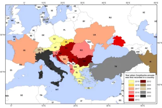
The oak lace bug (Corythucha arcuata, Say 1832 - Heteroptera: Tin- gidae), native to North America (Barber, 2010), is a new invasive alien species in Europe, spreading rapidly and causing foliage damage pri- marily of oak trees, potentially jeopardizing the long term health, pro- ductivity and stability of natural oak forests. Since it was first recorded in northern Italy in 2000 (Bernardinelli, 2000; Bernardinelli and Zan- digiacomo, 2000), the oak lace bug (hereafter OLB) has spread to most of the countries in South-East and Central Europe (Fig. 1), mostly passively by the traffic and to a lesser extent by the wind (Csoka et al., 2013; ´ Dobreva et al., 2013; Hraˇsovec et al., 2013; Tomescu et al., 2018;
Sotirovski et al., 2019; Mertelík and Liˇska, 2020). The pest arrived in the
* Corresponding authors.
E-mail addresses: anikoc@nimbus.elte.hu (A. Kern), hrvojem@sumins.hr (H. Marjanovi´c).
Contents lists available at ScienceDirect
Agricultural and Forest Meteorology
journal homepage: www.elsevier.com/locate/agrformet
https://doi.org/10.1016/j.agrformet.2021.108436
Received 4 January 2021; Received in revised form 23 March 2021; Accepted 8 April 2021
region of the Carpathian Basin from the Southeastern direction, where it was first recorded in 2013 in Croatia and Hungary (Csoka et al., 2013; ´ Hraˇsovec et al., 2013), affecting the valuable pedunculate oak forests of the Pannonian Plain. In recent years the infestation has gained mo- mentum (Simov et al., 2018; Cs´oka et al., 2020; Paulin et al., 2020), which might be promoted also by the drier weather and delayed arrivals of winter in the region in the last years (Csepel´enyi et al., 2017a).
All Central European native oaks are suitable hosts for the OLB, but it can occasionally develop on other hosts as well (Cs´oka et al., 2020). The outbreak populations in Central Europe were most commonly found on pedunculate oak (Quercus robur L.), Hungarian oak (Quercus frainetto Ten.), sessile oak (Quercus petraea (Matt) Liebl.) and Turkey oak (Quercus cerris L.) (Cs´oka et al., 2020). Damage to the leaves caused by the OLB (as a result of leaf-sucking) negatively affects leaf photosyn- thesis. Nikoli´c et al. (2019) found a 58.5% decrease in the rate of photosynthesis in the case of pedunculate oak, where the transpiration and stomatal conductance were decreased as well. The OLB, after overwintering in bark crevices and mosses on trees, has 2-3 new gen- erations during the year from April until October/November (Connell and Beacher, 1947). Foliar damage due to the intensive feeding of more generations becomes pronounced in the second part of the vegetation season as early discolouration of the upper surface of the leaves (Ber- nardinelli and Zandigiacomo, 2000; Paulin et al., 2020). In the case of heavy infestation, premature leaf and acorn abscission could occur, although the negative effects on tree regeneration have not been proven so far (Franjevi´c et al., 2018).
Unlike other disturbances (e.g. the gypsy moth (Lymantria dispar); de Beurs and Townsend, 2008; Csoka et al., 2015), the trees cannot recover ´ from the OLB caused damage still in the same growing season. As an alien species in Europe, the OLB has no significant natural predator or disease to control its population (Paulin et al., 2020). So far, only a few naturally occurring native enemies (Paulin et al., 2020) and entomo- pathogenic fungi (Kovaˇc et al., 2020) have been identified as potential candidates for use in biological control of the OLB population in the region. As a consequence, after establishing itself in a forest stand, the OLB unceasingly affects the oak trees and decreases tree productivity during many consecutive years. The long-lasting effects of such year-by-year reduced photosynthetic capacity due to the OLB are not yet known, however, it likely affects the carbon cycle, and the strong
infestations could contribute to increased tree dieback (Dietze and Matthes, 2014). Based on the in situ observations, during 2013–2019 there was no other significant pest or disease outbreak in the region affecting the oak forests with similar severity. The role of such in situ observations made by entomologists and foresters is indispensable but limited to the relatively low spatial and temporal resolution due to resource constraints (Chen and Meentemeyer, 2016).
Remote sensing provides a valuable tool for monitoring the plant status over large areas with regular spatial resolutions, short repeat time, and in some cases long time-series of data. The detection of forest disturbances by remote sensing has a broad literature (e.g. Fraser et al., 2005; Jin and Sader, 2005; Solberg et al., 2006; Spruce et al., 2011;
Griffiths et al., 2014; Meng et al., 2018; Imanyfar et al., 2019), and has also been used in national forest health and early disturbance moni- toring systems (Hargrove et al., 2009; Barka et al., 2018; Somogyi et al., 2018). Despite its relatively coarse spatial resolution, many studies have demonstrated the applicability of the high temporal resolution and exceptionally long datasets of the Moderate Resolution Imaging Spec- troradiometer (MODIS) for the regional-scale assessment of the insect-caused forest disturbances (de Beurs and Townsend, 2008;
Eklundh et al., 2009; Verbesselt et al., 2009; Bright et al., 2013; Olsson et al., 2016a, 2016b).
The Normalized Difference Vegetation Index (NDVI), derived from the measured reflectances in the red and near-infrared parts of the spectra, correlates strongly with the chlorophyll content and the photosynthetic activity of the leaves (Huete et al., 2002). Therefore, it is one of the most commonly used remote sensing vegetation index (VI) in detecting the infestation and studying the pest impact on the forest canopy (e.g. Spruce et al., 2011; Hargrove et al., 2009; Spruce et al., 2019). The pest damage is often quantified also with other spectral indices (de Beurs and Townsend, 2008; Eklundh et al., 2009; Verbesselt et al., 2009; Townsend et al., 2012; Sangüesa-Barreda et al., 2014), or by the reduction of some derived parameters like the Gross Primary Pro- ductivity (GPP), Net Primary Production (NPP), or Leaf Area Index (LAI) (e.g. Bright et al., 2013; Olsson et al., 2017).
Most of the existing studies on pest detection or pest disturbance assessment were based either on the yearly maximum VI (e.g. de Beurs and Townsend, 2008; Spruce et al., 2011) or the VI anomaly, i.e. the difference between the VI in the year when the pest was present and the
Fig. 1. Map of the spread of the oak lace bug in Europe and the Middle East. The map shows the years of the first records in the countries. (Source of data: https://gd.
eppo.int/taxon/CRTHAR/distribution, Sotirovski et al. (2019) for North Macedonia, and Mertelík and Liˇska (2020) for Czechia).
VI mean of the years preceding the pest disturbance serving as the reference (Eklundh et al., 2009; Townsend et al., 2012; Griffiths et al., 2014; Olsson et al., 2016b; Spruce et al., 2019). In such studies, the effects of the yearly meteorological and soil moisture conditions on the plant phenology are rarely taken into account explicitly. Recognizing the importance of the interannual variability of the phenology in the calculation of the pest-related VI anomaly, Ch´avez et al. (2019) pro- posed a method to reconstruct the annual phenology based on the fre- quency of the VI density, expressing the probability of the observed anomaly. Accounting for the effects of the weather and soil moisture on the interannual variability of VI is important in the pest damage assessment and modelling, particularly in the case of long-lasting in- festations. Decoupling of those effects in VI modelling so far has been rare and still presents a challenge.
The objective of the present study was to (i) identify forest areas with a high probability of OLB infestation by creating novel detection methods based on 20-year long MODIS NDVI data with 250 m spatial resolution for the transboundary area of Hungary and Croatia; (ii) create and validate NDVI models that will facilitate decoupling of the effects on the NDVI caused by the OLB from the effects caused by the year-to-year variability in weather, changing soil water content and forest manage- ment; (iii) assess and quantify the decrease in forest NDVI in the selected period of the growing season with respect to the different forest cate- gories and the share of oaks in a pixel; and (iv) map the OLB spread in the study area and estimate its speed based on the detected infested pixels.
2. Materials and methods 2.1. Study area
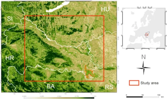
The target area of this study was the most OLB-infested parts of Croatia and Hungary, namely the Northeastern part of Croatia and the Southwestern part of Hungary, located in Central Europe (Fig. 2), be- tween 44.84–46.8◦N and 16.4–19.45◦E. The Hungarian part of the study area was selected as the area in Hungary which showed the highest infestation level in 2019 based on the in situ field observations (see below, Section 2.2). The Croatian part was selected to involve the starting location of the spread in Croatia, in the Spaˇcva forest (Hraˇsovec et al., 2013). Spaˇcva forest, as part of the Slavonian oak forests, is the largest pedunculate oak forest complex in Europe (Klepac and Fabijani´c,
1996) and served as an ideal breeding ground for the OLB showing high infestation intensity since 2016 (this study). According to the K¨oppen-Geiger classification scheme the climate of the area is warm temperate, with no dry season and warm to hot summers, corresponding to climate classes Cfb (in the West) and Cfa (in the East), respectively (Rubel and Kotek, 2010).
2.2. Presence of the OLB in the study area based on field observations In the Hungarian part of the study area, the OLB was first recorded in 2016 and the first larger infestation was reported in 2017 (Csepel´enyi et al., 2017b). In the Croatian part, the OLB was first found in Spaˇcva forest, where the spread started in 2013. Therefore, relying on the in situ observations of the study areas, the pre-“oak lace bug era” (hereafter PreOLB-era) of the applied MODIS dataset can be considered as 2000–2016 and 2000–2012, and the oak lace bug era (hereafter OLB-era) as starting from 2017 and 2013, in the case of Hungary and Croatia, respectively. The Hungarian in situ observations of the OLB in the forest compartments are recorded in the Hungarian National Forest Damage Registration System (NFK, 2020) regularly since 2019 and in the case of Croatia within the national system for Reporting and Forecasting in Forestry – IPP (Matoˇsevi´c, 2020) since 2016. The OLB monitoring in Croatia is conducted at the level of forest management unit (FMU, average area ~3 kha) on 68% of the forests (193 FMUs) in the Croatian part of the study area.
The records on the in situ presence of the OLB in the monitored forest compartments (Hungary) and FMUs (Croatia) were used to test the agreement with the detection results based on the methods presented in this work.
2.3. Remote sensing based dataset
To quantify the impact caused by the OLB in terms of remote sensing, official products created from the data of the MODIS sensor on-board satellite Terra were used with the finest available spatial resolution (Justice et al., 1998). We calculated NDVI from the Collection 6 MOD09Q1 surface reflectance product with 250 m spatial and 8-day temporal resolution (Vermote, 2015) for the study period of 2000–2019. The temporal composite MOD09Q1 contains atmospheri- cally corrected surface reflectances for the visible bands in 8-day pe- riods, resulting in 46 data per year for each pixel. To create NDVI the
Fig. 2. Map of the Hungarian and Croatian study areas located in Central Europe (the base of the map is a MODIS NDVI image from the beginning of September 2019). The Spaˇcva forest in SE Croatia, where the OLB was first detected in the study area in 2013, is delineated with a red line.
surface reflectances of Band-1 (ρRED, in visible red) and Band-2 (ρNIR, in near-infrared) of the sensor were used, where NDVI is defined as (ρNIR - ρRED)/(ρNIR +ρRED). The Hierarchical Data Format (HDF) files of the MOD09Q1 product contain Julian date information and State and Quality Control (QC) flags as well at the pixel-level, where the time- stamp of the data refers to the exact dates when they were measured.
Data for the tile h19v04 were downloaded from NASA LP DAAC (LP DAAC, 2020).
Processing all of the datasets of the present study and execution of the calculations were performed using the Interactive Data Language (IDL) version 8.6 (Harris Geospatial Solutions, USA), and STATA 14.2 (StataCorp., USA).
The flowchart of the applied methodologies presented in the following sections is shown in Fig. S1 in the Supplementary Material.
2.3.1. Creating smoothed NDVI time-series from the raw MODIS reflectance dataset
The first step in obtaining a quality filtered and smoothed NDVI time- series at a regular grid with 8-day temporal resolution was the pre- processing of the raw dataset containing information on the exact Julian dates of the reflectance measurements, based on the work of Kern et al., 2016 and 2020, where only data with the strictest quality criteria were kept. To avoid any misleading and non-realistic sudden NDVI decrease due to the presence of unrecognized and incorrectly quality flagged atmospheric effects (such as high aerosol content, presence of thin cirrus, sub-pixel clouds, etc.), the Best Index Slope Extraction (BISE) method (Viovy et al., 1992) was applied at the pixel-level. The quality checked and gap-filled NDVI dataset was then resampled into daily resolution using linear interpolation, where the actual Julian dates of the measurements were taken into account. Then, the widely used Savitzky-Golay filter (e.g., Chen et al., 2004; Eklundh et al., 2009;
Spruce et al., 2011) was applied with a moving time window of 15 days to smooth the dataset using the built-in IDL SAVGOL and CONVOL routines. From the smoothed daily resolution dataset only 46 data points were preserved for each year, corresponding to the middle of the orig- inal 8-day periods. This smoothed NDVI dataset at a regular 8-day res- olution time step served as the basis for our investigations.
2.4. Meteorological and soil water content dataset
To investigate the effects of the weather and other environmental conditions on the vegetation during the late summer meteorological data of the FORESEE database (Dobor et al., 2014) and soil water con- tent of the ERA5-Land dataset (Balsamo et al., 2009) were used.
FORESEE contains observed and projected daily maximum/minimum temperature [◦C] and precipitation fields [mm day-1] for the wide region of the Carpathian Basin (42◦35’–51◦05’N, 10◦55’–28◦05’E) on a regular grid with a spatial resolution of 1/6◦×1/6◦, covering the 1951–2100 period. Daylight average shortwave radiative flux (in other words global radiation; [W m−2]) was calculated on the same grid using the MTClim model (Thornton et al., 2000), and multiplied with the corresponding day length (in seconds) to get the values in MJ m−2 day-1. The three-hourly ERA5 Land volumetric soil water [m3 m−3] were down- loaded from the Copernicus site (CCCS, 2019) with 0.1◦×0.1◦spatial resolution for two different soil layers (3rd and 4th layer at 0.28–1 m and 1–2.89 m depth, respectively) of the study area, and were used to create daily mean soil water content (SWC) values during 2000–2019.
The daily data stored at the original grid of FORESEE and ERA5 were resampled to the finer grid of the MODIS products using linear inter- polation. In the case of temperature and precipitation, the resampling was performed based on the methodology of Kern et al. (2016), where the elevation of the pixels was also taken into account.
2.5. Land cover datasets with spatially explicit tree species distribution information
2.5.1. Land cover datasets
Since the study area is part of two countries, two different national land cover datasets were utilized. For Hungary, the National Ecosystem Base Map land cover dataset of the NOSZT¨ EP project (Tan´ ´acs et al., 2019; http://web.map.fomi.hu/nosztep_open/) was used to distinguish the land cover types with the available species information. This newly published land cover dataset (hereafter referred to as NOSZT¨ EP) has 56 ´ different categories at Level-3 with a 20 m spatial resolution, stored in Lambert Azimuthal Equal Area projection, covering entire Hungary. In the present study, this Level-3 dataset was at first reprojected to WGS-84, and then overlapped with the 250 m resolution (QKM) MODIS grid. This enabled the calculation of the share of each of the 56 NOSZT¨ ´EP Level-3 categories within every MODIS pixel. Table S1 in the Supplementary Material lists the Level-3 categories of the NOSZT¨ ´EP’s Forest and Woodlands (Level-1) category, as well as the number of the QKM pixels with respect to the predefined minimum share of a given Level-3 category within the pixels. The base year of the thematic dataset was 2015, which was partially improved by high-resolution remote sensing data (Sentinel-1 and -2) from the year 2017 (Tan´acs et al., 2019). The land cover map of the Hungarian study area at the QKM grid with the dominant NOSZT¨ EP category of each pixel is shown in Fig. S2a, ´ while the corresponding legend is presented in Fig. S2b in the Supple- mentary Material.
In the case of Croatia, the main source of the land cover data was the database HˇS Fond of the Croatian Forests Ltd. The HˇS Fond is the national forestry database containing data from both state and private forests including spatial information on forest area division down to forest sub- compartments as elementary units. Basic data on forests from the HˇS Fond database are also available to the public (http://javni-podaci.
hrsume.hr/). The following data from the HˇS Fond database were used for all forest sub-compartments (excluding those containing stands younger than 20 years or those categorized as shrubs): volume of standing live trees, estimated annual increment, year of harvesting/
thinning/salvage logging, and volume of cut trees, all according to the different tree species. The living tree volume and increment are measured once every ten years in preparation of the forest management plans. Using the above data, we modelled the volume of the living trees (at species level) by adding the estimated increment to the initial volume and subtracting the harvest recorded in that year. The result was for every forest sub-compartment, the sequence of annual values for the living trees volume, increment and harvest at the species level (expressed in m3 ha-1) for all years of the study period, namely 2000–2019.
In the next step, the forest sub-compartment polygons were inter- sected with the MODIS QKM pixel grid projected in the local HR_ETRS89/TM geographic reference system (EPSG: 3765) using QGIS 3.10.2 with GRASS7.8.2 GIS software (an example shown in Fig. S3 in the Supplementary Material). Finally, the forested area, the volume, the increment, and the harvest (all by tree species) were calculated for every MODIS QKM pixel in every year during the period 2000–2019.
2.5.2. Pixel selection
Pixel selection criteria for the Hungarian and Croatian parts of the study area was mostly uniform, but also included some additional country-(i.e. dataset)-specific criteria. The uniform part of the pixel se- lection procedure consisted of two steps. In the first step pixels not reaching the minimum of 95% forest cover were discarded. This step was applied to secure that the signal from the non-forest areas (in particular due to croplands and grasslands) remains low. In the second step, the forest share of the side-neighbouring pixels to those that passed Step 1 was checked, and those which did not reach the minimum forest cover of 60% were also excluded. This filtering criterion was applied due to the known geolocation inaccuracy of the MODIS measurements
(Wolfe et al., 2002) and due to the artefacts of the gridding procedure (Tan et al., 2006) and possible re-projection inaccuracies. The used 60%
threshold was chosen based on a preliminary assessment of the potential impact of the above-mentioned confounding effects and the need to retain as many pixels as possible.
For the Hungarian part of the study area, an additional filtering step was designed due to the lack of forest management data. The possible forest management events (e.g. stand harvesting) or possible massive abiotic disturbances that could have occurred (e.g. windthrow) in a pixel were detected based on the mean NDVI of the main part of the growing season (NDVI19–31; 19th to 31st MODIS 8-day period, corresponding to 25 May – 5 Sep). The starting and the ending 8-day period of the main part of the growing season were determined to reflect a general period when the phenology of all forest pixels in the study area (and during all years of the study period) has surely passed the End of Green-up (EoG) in spring but has not reached the Onset of Senescence (OoS) in autumn.
The latest EoG and the earliest OoS were calculated using the 20% cut- off method (Hargrove et al., 2009; Shen et al., 2015; Wang et al., 2018;
Kern et al., 2020). The threshold of the NDVI19–31 was set to 0.8 based on the distribution of the NDVI19–31 values during the PreOLB-era. Pixels below the threshold in any of the years during the investigated 2000–2019 period were excluded from the dataset.
For the Croatian part data on standing tree volume and annual harvests at the species level were available for every pixel during the period 2005–2019. Consequently, the effects of forest management were addressed by excluding all pixels having total harvesting intensity in the period 2005–2019 above 35% or those containing less than 50 m3 ha-1. 2.5.3. Categorization of the selected pixels according to dominant tree species
Tree pests and diseases frequently occur exclusively or, as is the case with the OLB, have a preference for particular tree species. The observed damage from the pest is generally proportional to the share of the tar- geted tree species and the density of the pest (severity of the “attack”).
Therefore, the share of the oaks (Quercus sp.) and other accompanying tree species had to be considered in every pixel.
Table 1 lists the created forest groups indicating the number of pixels within each group for each country. For Hungary, the pixel categoriza- tion was based on the share of areas of NOSZT¨ ´EP Level-3 categories.
Pixels having at least 95% of the area covered by the corresponding forest type were selected for this study. Categorization with respect to forest groups in the case of Croatia was based on the volume shares of different tree species. Pure oak groups contained pixels with >85%
share of corresponding oak species in the total volume of live trees in a pixel. Pure groups of oak with other species (common hornbeam or narrow-leaved ash) contained 50–85% of oak and the other species was by its volume share second after oak. Fig. 3 shows the map of the selected pixels by the defined forest groups.
Pure groups contain pixels in which only one forest type is predom- inantly (>95%) present (Hungary), or the volume share of the dominant tree species in a given forest group is greater than 50% (Croatia). It is important to keep in mind that, due to the high degree of land cover diversity and the coarse MODIS resolution (250 m), by using only Pure groups we would discard a lot of forested pixels containing more forest types. To avoid this, we created and tested two extended groups: the Oaks above 50% share and the Oaks above 20% share. Pixels dominated by pubescent oak (with 95% share), and in the case of Croatia also by Turkey oak were dropped from the study due to the low pixel numbers.
The additional group Oaks below 10% share contained pixels having less than 10% oaks and ashes (Fraxinus sp.) and served as a control group.
The reason behind excluding narrow-leaved ash was the emergence of the ash dieback fungus (Hymenoscyphus fraxineus, previously known as Chalara fraxinea) in Central Europe, the first time recorded in Hungary in 2008 (Szab´o, 2008) and in Croatia in 2011 (Bari´c et al., 2012;
Matoˇsevi´c, 2012).
Finally, the Leftover forest group contained forested pixels which did not meet the selection criteria and served only for the visualization of the forested area.
2.6. Identification of pixels with OLB-like damage based only on the remote sensing data (RS method)
The identification of the pixels with typical OLB-like damage was based on the observable NDVI decrease in a pre-defined period (see below) due to damage from the feeding activity of the OLB. This be- comes observable by remote sensing as the decrease in the NDVI already in late July. The NDVI decrease becomes strong from the second part of August when the possible second generation of the OLB emerges (Franjevi´c et al., 2018). Table 2 presents the exact dates of the MODIS 8-day periods during the year relevant from the remote sensing perspective to the monitoring of the OLB damage.
Considering the above, the strongest NDVI decrease (observed as the sharpest NDVI decrease due to the OLB) happens during the late summer and the beginning of autumn (~30th to 33rd MODIS 8-day period during the year). The decrease in the NDVI continues afterwards as well, but it is difficult to attribute it solely to the OLB. The earliest recorded onset of senescence in the study area in the PreOLB-era was the 33rd 8- day period (starting from ~ 14st Sept). To avoid the possible effects of early senescence, the identification of the OLB presence was based on the decrease in the average NDVI during the 30th to 32nd 8-day period (21st of Aug – 13th of Sept, hereafter period30–32). The application of averaging the three consecutive 8-day periods was chosen also to minimize the false identification of pixels as a consequence of any remaining, unidentified noise in the NDVI dataset due to clouds, atmo- spheric or angular effects.
The RS method for identifying disturbances that could be related to the OLB consisted of two conditions. The basic assumption was that the observed NDVI of a given (i,j) pixel shows negative NDVI anomaly during the investigated period30–32 of the given year in the forms of:
NDVIi,j,p,y<MeanNDVIi,j,p,PreOLBforp=30− 32, (1)
where MeanNDVIi,j,p,PreOLB is the multiannual mean NDVI for the indi- cated periods during the PreOLB-era, and NDVIi,j,p,y are the mean values of the processed NDVI dataset at the pixel-level in the indicated 8-day Table 1
The number of the selected MODIS QKM pixels according to the defined forest groups.
Investigated species groups n -
Hungary n - Croatia Pure groups
Pure pedunculate oak (Q. robur) N/A 390
Pedunculate oak with narrow-leaved ash (Q. robur &
F. angustifolia) 150 1467
Pedunculate oak with common hornbeam (Q. robur &
C. betulus) 136 1606
Sessile oak with common hornbeam (Q. petrea &
C. betulus) 491 131
Turkey oak (Q. cerris) 476 31
Pubescent oak (Q. pubescens) 23 4
Sessile oak with common beech (Q. petrea & F. sylvatica) N/A 1215
Pure ash (F. angustifolia) N/A 114
Pedunculate oak (mixed) a 442 N/A
All oaks b 2048 N/A
Extended groups
Oaks above 50% share (Quercus share >50%) 5,217 8,711 Oaks above 20% share (Quercus share >20%) 7485 17,013 Additional groups
Oaks below 10% share 5775 5013
Leftover forested 18,146 18,322
N/A Due to differences between the Hungarian and Croatian forest datasets the group is not applicable for this country.
aAll NOSZT¨ ´EP Level-3 categories with pedunculate oak in a pixel combined.
b All NOSZT¨ EP Level-3 categories with any kind of oak in a pixel combined. ´
periods (p) of the investigated year (y), respectively. The second crite- rion was based on the mean difference during the PreOLB-era between the yearly MaxNDVIi,j,19–29,y and MinNDVIi,j,30–32,y values (where the latter is the yearly minimum NDVI value of the period30–32), indicated as MeanNDVIdiffi,j,PreOLB. This criterion is defined as:
NDVIi,j,p,y<MaxNDVIi,j,19−29,y− MeanNDVIdif fi,j,PreOLBforp=30− 32, (2) where:
MeanNDVIdif fi,j,PreOLB=mean(
MaxNDVIi,j,19−29,y− MinNDVIi,j,30−32,y
). (3) In the case when both criteria are met, the pixel is classified as damaged for the year in question, likely by the OLB. We assigned a continuity flag (hereafter C-flag) to each pixel containing information about the continuity of the disturbance detection in the subsequent years of the OLB-era. Namely, C-flags are: 1 – not detected during the OLB era;
2 – damage detected intermittently in some years; 3 – detected contin- uously every year since the first year of detection.
2.7. Identification of pixels with OLB-like damage using NDVI model residuals (MR method)
The assessment of the OLB infestation required decoupling the OLB effect on the NDVI from the effects of the main meteorological and environmental variables as well as the effects of other pests and man- agement. To do this, prognostic multiple linear models for the yearly mean NDVI during the investigated period30–32 (hereafter NDVI30–32) were constructed (Section 2.7.1). The model residuals were used to identify forested pixels which can be linked to the damage from the OLB infestation (Section 2.7.2).
The MR method for the OLB detection is based on the assumption that the distribution of the residuals of the NDVI model does not change with time if the independent variables remain within their usual (e.g.
calibration) range. If there is a sudden change in the distribution of the Fig. 3.Map of the used QKM pixels after the strict filtering procedure in the different Pure species categories in the study area. (Pixels of the Extended and Additional groups are not shown)
Table 2
The ordinal number of the MODIS 8-day periods during the OLB affected period of the year, corresponding Julian days of the year (DOY), dates, and comment relevant to the OLB detection.
Number of the
8-day period Julian
days Date Description/Comments
25th 193 –
200 12–19th of July Possible appearance of the second OLB generation
26th 201 –
208 20–27th of July
27th 209 –
216 28th of July – 4th
of August The OLB caused NDVI decrease might become noticeable
28th 217 –
224 5–12th of August
29th 225 –
232 13–20th of August
30th 233 –
240 21–28th of
August Investigated period: used in identification and modelling
31st 241 –
248 28th of Aug. –
5th of Sept. Investigated period: used in identification and modelling
32nd 249 –
256 6–13th of
September Investigated period: used in identification and modelling
33rd 257 –
264 14–21st of
September The earliest recorded OoS during the PreOLB-era
34th 265 –
272 22–29th of
September Average time for the OoS during the PreOLB-era
model residuals, i.e. if the model performance suddenly becomes considerably worse while the independent variables are within the usual range, then this is an indicator that some new agent (OLB) additionally affecting the NDVI has appeared.
Using only data from the PreOLB-era to avoid the influence of the OLB, the constructed models were calibrated and then validated by applying the leave-out-one-year (LOOY) cross-validation technique (Santos et al., 2011). In the LOOY validation, the model is calibrated with a dataset from which one calendar-year of the data are year-by-year omitted. Model predictions were then tested against the observations in the year that was left out, which was repeated for all years of the vali- dation dataset. When used for prediction, data of the entire PreOLB-era were used for model calibration and the model was then applied for the whole study period (2000–2019).
The studied parts of Hungary and Croatia belong to two different biogeographic regions (the Pannonian and the Continental, respec- tively), where the border between the two biogeographical regions corresponds to the county borders. To reflect the differences due to the geography and the weather, but also due to the land cover datasets and forest management practices, country-specific NDVI30–32 models were constructed.
2.7.1. Building of the NDVI30–32 model
The NDVI models were build using two kinds of predictor variables at the pixel-level: i) meteorological and environmental variables: daily minimum and maximum temperature (Tmin and Tmax); the amount of available shortwave solar energy (Rad); precipitation (Prec); and soil water content at two layers (SWC3 and SWC4); and ii) mean NDVI of periods 25–26 (i.e. before the assumed start of the observable NDVI decrease; hereafter NDVI25–26). In the case of the meteorological and environmental variables, the mean (and in the case of precipitation the total) of the 16 days were used. The NDVI25–26 served as a proxy variable for non-OLB pest damage and forest management activities, as most of the non-OLB pest activity (e.g. defoliation of oaks by Lymantria dispar, or the effects of infestation with the powdery mildew) or management activities (e.g. thinning) reflect on the NDVI25–26.
The general theoretical form of the considered NDVI30–32 model based on the different averaging periods (AP) of the applied variables was:
where TmaxAP, TminAP, PrecAP, RadAP, SWC3AP, SWC4AP are the pixel- level mean of the maximum and minimum temperature, precipitation, radiation, and soil water content at two different layers for a given AP, respectively, and αAP, βAP, γAP, δAP, εAP, ζAP, and η are model coefficients.
The general model (Eq. (4)) has a very large number of predictor vari- ables and would suffer from issues such as co-linearity, overfitting, and lack of interpretability, thus the number of variables in the model had to be reduced. The reduction of the general model by identification of the smallest set of most important variables and time periods was based on the Lasso approach, separately for each country.
The Least Absolute Shrinkage and Selection Operator (Lasso) was used for selecting the optimal set of predictor variables. The Lasso is a regularized regression method which applies λ1 norm penalization to achieve sparse solutions (Tibshirani, 1996). This technique is suitable for high-dimensional cases where the number of independent variables is large (Ahrens et al., 2020). The selection of the best set of predictor variables was made using STATA 14.2 and the program cvlasso, which is part of the package lassopack (Ahrens et al., 2020). The applied cvlasso
uses k-fold cross-validation (in our case, each fold was defined by the calendar year) for selecting the penalty level parameter lambda, which optimizes out-of-sample prediction performance by minimizing the mean-squared prediction error. Bayesian Information Criterion (BIC), root mean square error (RMSE), mean absolute error (MAE), bias, and coefficient of determination (Pearson R2) were used for the assessment of the goodness of the model.
In the next step, the set of independent variables obtained with cvlasso was used to perform the model calibration and validation with the ordinary least square regression (OLS). The initial set of predictor variables was further reduced by applying a procedure that is similar to the backward stepwise regression. At first, the model obtained with cvlasso was calibrated using the entire PreOLB data and all non- significant (p < 0.05) variables (if any) were removed one-by-one until only those significant remained. Then, the model was validated using the LOOY cross-validation technique (Santos et al., 2011) based on the PreOLB part of the dataset. If some of the variables became non-significant (p <0.05) at any step of the validation, that variable was removed (starting with the least significant one) and the procedure was repeated until all variables were significant at all times. The removal of the least significant predictor variables continued, even if all variables were significant (p <0.05), up to the point when the model with the smallest (or most negative) cross-validation BIC, RMSE, MAE, bias and the highest cross-validation R2 were identified. This extension of the Lasso procedure enabled us to find an optimal model with the smallest number of independent (and highly significant) variables and best model performance on the validation dataset. The final models were then calibrated using the PreOLB part of the dataset (2000–2016 for Hungary and 2000–2012 for Croatia) and used for the calculation of the Z-score (see next section). The model coefficients and the performance statistics were calculated independently using the IMSL_multiregress function in IDL and regress function in STATA to assure reliable and error-free results.
2.7.2. Identification of the OLB infested pixels based on the NDVI30–32
model residual Z-score
The Z-score, or standard score of a data point, is the distance of the data point from the population (sample) mean, expressed in units of standard deviations. Assuming the model residuals are normally
distributed, the residual Z-score can be used in outlier detection since the Z-scores of less than -3 or greater than 3 are typically considered outliers (Misra et al., 2020). For a model that is not biased and which has nor- mally distributed residuals, the share of residuals with z < -3.09 would be 0.001, or 0.1%. According to this, the z =-3.09 of the model residuals during the OLB-era was used as a threshold for the detection of outlier pixels with unexpectedly negative residual. The unusually low observed NDVI, much lower than expected (modelled) after accounting for the variability caused by the meteorology, soil water content and NDVI25–26, served as an indicator of the damage that could be associated with the presence of the OLB. Therefore, all pixels with a residual Z-score less than -3.09 were identified as affected by the OLB. The effects of other pests, management activity, or natural disturbance were in most cases already visible on the NDVI25–26 and therefore have been accounted for in the model. This emphasizes the essential role of the NDVI25–26 in the NDVI30–32 modelling. The remaining, unaccounted negative residuals may be (with high probability) attributed to the OLB.
The values of the model residuals during the PreOLB-era (i.e., the years 2000–2012 for Croatia or 2000–2016 for Hungary) were used for NDVI30−32=∑
AP
(αAP⋅TmaxAP+βAP⋅TminAP+γAP⋅PrecAP+δAP⋅RadAP+εAP⋅SWC3AP+ζAP⋅SWC4AP) + η⋅NDVI25−26+constant, (4)
the calculation of the mean and the standard deviation of the model residuals at the pixel-level. The Z-score of the model residual for an (i,j) pixel and y year was calculated as:
zi,j,y= (
ri,j,y− ri,j,PreOLB
)
si,j,PreOLB
, (5)
where ri,j,PreOLB and si,j,PrePLB is the mean and standard deviation of the model residuals during the PreOLB-era for the pixel (i,j).
Considering that the number of data points (years) per pixel is small, it could be expected that the assumption of the normality of the re- siduals’ distribution at the pixel-level would not be always met. How- ever, given that the number of the pixels is large, the violation of the normality assumption at the pixel-level may be acceptable (e.g. Zeller and Levine, 1974), especially if the overall distribution of the residuals during the PreOLB-era is close to normal distribution. Provided that the residuals are normally distributed and given that the share of pixels with z <-3.09 under the normal curve is 0.1%, the probability of error (false-positive) in our case would be 0.1%. If the share of the pixels identified as outliers during the PreOLB-era was sufficiently close to the theoretical value of 0.1% we may assume, in line with Zeller and Levine (1974), that possible deviations of residuals from normal distribution did not affect significantly the results.
Assessment of the goodness of the used Z-score threshold value regarding the false-negative detections could not be as direct as in the case of false-positive. Therefore we investigated the evolution of the Z- score of the infested pixels’ residuals from the year when a pixel has been detected as infested by the MR method for the first time during the OLB- era. The year of the first detection was marked as year zero, and only pixels with C-flag 3 were considered. If the selected threshold (-3.09) is adequate, the average Z-score in the year preceding the first year of detection (i.e. in the year =-1) should not be significantly different from zero.
2.8. Assessment of the OLB-caused NDVI decrease
For a given year y in the OLB-era the model bias (biasy) is the result of two causes: bias due to inherent model limitations (bias0,y) and the additional bias (biasOLB,y) that is caused by the OLB related decrease in NDVI:
biasy= bias0,y+ biasOLB,y. (6)
It should be noted that the above equation is a simplification as it does not take into account the possible effects of the meteorology on the OLB activity/abundance. For the years of the PreOLB-era the biasOLB,y is zero (by definition), therefore Eq. (6) becomes:
where n is the number of pixels.
The average decrease of the NDVI30–32 of the detected pixels that is caused by the OLB in a given year corresponds to the mean residual of the infested pixels, corrected for the inherent model bias for that year (bias0,y). The model bias0,y could not be calculated for the years in the OLB-era, therefore it was approximated with the average of the model biases during the PreOLB-era (Eq. (7)), obtained by the LOOY cross- validation. The average decrease in NDVI30–32 (D30−32,y) of the OLB infested pixels in a given year y is calculated as:
D30−32,y=residualinfested,y− bias0,y≈residualinfested,y− biaspreOLB, (8) where residualinfested,y is the mean model residual of the infested pixels in year y, residualinfested,y is the cross-validation mean bias during the Pre- OLB-era. The standard error (seD,y) of the D30−32 in a year y is:
seD,y=
̅̅̅̅̅̅̅̅̅̅̅̅̅̅̅̅̅̅̅̅̅̅̅̅̅̅̅̅̅̅̅̅̅̅̅̅̅̅̅̅̅̅̅̅̅̅̅̅̅̅̅̅̅̅̅̅̅̅
se2residualinfested,y+se2bias,PreOLB
√ (9)
where seresidualinfested,y is the standard error of the mean residual of the infested pixels in a given year y and sebias,PreOLB is the standard error of the mean bias during the PreOLB-era, obtained with cross-validation.
2.9. Comparison of the RS and MR detection and agreement with the in situ records
The agreement of the results of the RS and MR detection methods were compared with McNemar’s test for the equality of the marginal frequencies (McNemar, 1947). For pixels detected as infested, a status of the detection in the following year was examined to check the agree- ment between the methods and the continuity of the detection.
The validation of the methods in the strictest sense, where each MODIS pixel area corresponding to the same validation area would be monitored every year and the presence or the absence of the OLB would be recorded, was not possible because such data do not exist. Therefore, the existing albeit very short (Hungary) or coarse (Croatia) records of the in situ OLB presence were used for the comparison with the detection results of the RS and MR methods. The McNemar’s test was again used for testing the differences between the RS and MR detection methods against the records of the in situ OLB presence.
2.10. Locating the origin of the infestation and calculating the rate of the OLB spread
Using the RS and MR methods for identification of the infested pixels we created maps showing the detected spread of the OLB infestations based on the year of the first detection. Also, both the RS and MR methods were used to reconstruct the origin of the OLB spread in the study area and to test the agreement with the field observations. The origin of the OLB spread was determined as the centroid (geographical mean) of the infested pixels detected in 2013 (as the first year) in the area of Spaˇcva forest. The maps and calculations were made with QGIS 3.10.2 with GRASS 7.8.2 and ESRI ArcGIS 10.1 Desktop software.
By setting the origin of the infestation as the centre of the coordinate system, the mean radial distance of the newly infested area (pixels) was calculated for every year using only continuously detected pixels (with C-flag 3). The mean annual radial speed of the spread (in km y−1) for a
given year was calculated as the difference between two consecutive mean radial distances divided by one year.
3. Results
3.1. Detecting pixels with OLB-like damage based on the RS method Using the RS method we discriminated the possible infested pixels from the probably not infested ones. However, it is important to note that at this point we still cannot claim that the detected NDVI decrease of a pixel is only attributed to the OLB or if other biotic or abiotic factors biasy= bias0,y=1
n
∑(NDVImodelled,30−32,y− NDVIobserved,30−32,y
),y ∈ PreOLB− era (7)
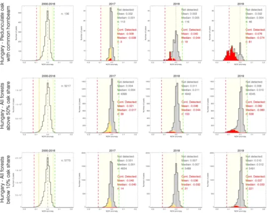
also significantly contributed to the decrease. Figs. 4 and 5 show the NDVI30–32 anomaly distributions (grey) by years during the OLB-era for three main species groups in Hungary and Croatia, respectively. The NDVI30–32 anomaly distribution during the PreOLB-era is shown in the first plot of the species groups as a reference, followed by the distribu- tions for all years of the OLB-era (2016–2019 for Hungary and 2013–2019 for Croatia). Distributions of the pixels which were detected as continuously infested since the first year of detection (C-flag 3), and those detected intermittently (C-flag 2), are indicated separately with red and yellow colour, respectively. Dashed and dotted lines indicate the 0.1 and 1 percentile range of the overall NDVI30–32 distribution during the PreOLB-era. In the lack of the Pure pedunculate oak category in Hungary, the Pedunculate oak with common hornbeam group is shown, as it is the one with the highest share of pedunculate oak. Histograms of the other species groups are presented in Figs. S4 and S5 in the Supple- mentary Material.
From the NDVI anomaly distributions (Figs. 4 and 5) it is visible that in the case of the forests with a significant share of oaks species the distribution started to shift toward the left into the negative anomaly range with time. The start of the observed shifts occurred approximately one year after the OLB has been found in situ for the first time in the study area. The magnitude of the observed anomalies is more pro- nounced (left of 0.1 percentile of the PreOLB-era) for the forest cate- gories having the largest oak share, but not observed for the forests with less than 10% oak share. In the third year, an obvious second peak of the anomaly distribution appeared which became more and more pro- nounced with the spread of the OLB during the years. While in the Hungarian part of the study area the OLB infestation started in 2017, in Croatia it caused serious infestation already in 2016, with a maximum NDVI30–32 anomaly of -0.124 for Pure pedunculate oak forests recorded in 2018. The control group Oaks below 10% share showed less interannual variability in distribution. Although there were some detected pixels with OLB-like disturbance, the NDVI30–32 anomaly distributions showed no shifts in distribution during the OLB-era.
The NDVI30–32 values of the detected pixels were affected by the OLB and at the same time by the weather and environmental conditions. The true effects of the OLB are clearer in “good years” (from the perspective of the effect of the meteorology on the vegetation state; see Kern et al., 2017; Ani´c et al., 2018) when the overall NDVI anomaly is positive, as was the case in Croatia (Fig. 5). There, the pixels identified as not infested in 2015 (and to a lesser extent in 2016) showed a strong overall positive anomaly, but those detected as infested showed strong negative anomaly. Similar could be observed in 2019 in the case of Hungary (Fig. 4). An interesting year is 2017, which may be characterized as a
“bad year” for oak forests in Croatia since even the not detected pixels exhibited negative anomaly. There we can see a relatively higher amount of not continuously detected pixels (C-flag 2, shown in orange in Fig. 5). Moreover, we can observe a slight increase of the not continu- ously detected pixels in the control group as well (Oaks below 10% share, Fig. 5), which could be an indicator of the increased uncertainty in the ability of the RS identification method in “bad years”.
Fig. 6a and b show the mean NDVI curves (trajectories) of the detected pixels with C-flag 3 in each year in the case of the Pure pedunculate oak with common hornbeam of Hungary and the Pure pedun- culate oak category of Croatia, respectively, relative to the multiannual mean NDVI curves during the corresponding PreOLB-eras. The seasonal NDVI decrease in late summer and early autumn is obvious after the OLB was found in situ for the first time. Both the presented NDVI anomaly histograms (Figs. 4 and 5) and the mean NDVI curves (Fig. 6) indicates that from the time when the OLB arrives to an area it takes approxi- mately 2–3 years for the NDVI decrease to reach its maximum, after which, it seems that it does not decrease further.
3.2. Modelling NDVI30–32
The created models were built for the Oaks above 20% share forest group, separately for each country, for reasons of simplicity and robustness. The aim was to create a method that could be generally Fig. 4. Distributions of the NDVI30–32 anomalies showing the progression of the OLB infestation detected continuously (red) or intermittently (orange) in the forest categories Pedunculate oak with common hornbeam (top row), Oaks above 50% share (middle row), and Oaks below 10% share (bottom row) for the Hungarian part of the study area. (For interpretation of the references to color in this figure legend, the reader is referred to the web version of this article.)
applied and easily reproduced, also because the tree species distribution is rarely available with a high spatial and accurate temporal resolution.
The equations of the created Lasso models (M1 for the Hungarian and M2 for the Croatian part of the study area) are shown in Table 3. The statistics of the model coefficients (estimates, standard errors, t-statis- tics, p-values) are presented in Table S2 in the Supplementary Material.
The parameters of the presented models were found to be significant at p <0.0001 level.
After building a country-specific model for each country, the same models with the same coefficients of the linear regression were applied to the separate forest groups. Table 4 shows the performance metrics of the NDVI30–32 models M1 and M2, during the PreOLB-era, which have been calibrated using the data for pixels in the Oaks above 20% share category and then cross-validated on the different forest groups of Hungary and Croatia, separately. Based on the calibration, the Hun- garian M1 model showed an R2 of 0.5569 with 0.0186 RMSE, 0.0137 Fig. 5. Distributions of the NDVI30–32 anomalies showing the progression of the OLB infestation detected continuously (red) or intermittently (orange) in the forest categories Pure pedunculate oak (top row), Oaks above 50% share (middle row), and Oaks below 10% share (bottom row) for the Croatian part of the study area. (For interpretation of the references to color in this figure legend, the reader is referred to the web version of this article.)
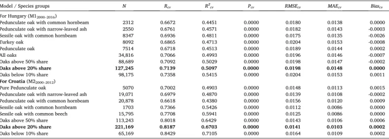
MAE, and 0.0000 bias, while the Croatian M2 model had an R2 of 0.6912 with 0.0136 RMSE, 0.010 MAE, and 0.0000 bias. In the case of Hungary, the results of cross-validation based on the 2000–2016 PreOLB-era show 0.44–0.50 cross-validated R2 values with an RMSE between 0.017 and 0.020. Amongst the pure forest groups, the best model performance was observed in the case of Sessile oak with common hornbeam group, while the poorest in the case of the pedunculate oak-dominated groups. In the case of Croatia, the cross-validated R-values were in the range of 0.66–0.82, with RMSE values between 0.011 and 0.016. The results show an unequivocally better model performance of the Croatian model than the model for Hungary.
3.3. Detecting pixels with OLB-like damage based on the MR method In every year of the OLB-era, all pixels have been categorized into infested or not infested based on the Z-score of the model residual (see Section 2.7.2). The share of pixels identified as damaged with the MR method during the PreOLB-era on the modelling dataset (Oaks above 20% share) ranges from 0% to 0.79% with the mean (std. err.) of 0.12%
(0.05%) in the case of Hungary. In the case of Croatia, the range was from 0% to 0.18% with the mean (std. err.) of 0.05% (0.02%). Those values represent the independent estimate of the expected share of false- positive detections with the MR method. The obtained shares are in line with the theoretical value for the expected false-positive OLB-detection, which is 0.1%, based on the selected Z-score threshold (Section 2.7.2, z
=-3.09).
Fig. 7 shows the temporal evolution of the Z-score distributions with respect to the relative years of detection in the case of the Oaks above 20% share forest group, separately for Hungary and Croatia. The dis- tribution of the Z-score values for the relative year of detection of -1 (one year prior to detection) is in both cases centred almost at zero and similar to the Z-score distributions of the previous years. This is a strong indicator that, with the selected z =-3.09 threshold the number of false- negative detections could be considered negligible.
Fig. 8 shows the yearly distributions of the model residuals (i.e. the observed NDVI - modelled NDVI) for the same species groups as in Figs. 4 and 5, with the box-whisks plot indicating the yearly mean, 1, 5, 25, 50, 75, 95 and 99 percentile values. It should be emphasized that the distributions in the PreOLB-era shown in Fig. 8 correspond to the dis- tribution of the residuals in model validation. Box-plots of the pixels
Fig. 6. Multiannual mean (MAM) and yearly mean NDVI curves of the detected pixels with C-flag 3 for the Pedunculate oak with common hornbeam category of Hungary (a) and the Pure pedunculate oak category of Croatia (b), where the MAM is based on 2000–2016 and 2000–2012, respectively. The range created from the average of the absolute minimum and maximum NDVI of each pixel in each period during the PreOLB-era is also indicated with light yellow shading (where averaging is over 136 and 390 pixels, respectively for the two countries). (For interpretation of the references to color in this figure legend, the reader is referred to the web version of this article.)
Table 3
Equations of the constructed Lasso models (M1 and M2) of forest NDVI30–32
calibrated with the data of the PreOLB-era (2000–2012/16) for the Hungarian and Croatian part of the study area, separately. (Subscripts denote MODIS 8-day periods; see Table S3 in the Supplementary Material).
Model Equation of the model For Hungary
M12000–2016 NDVI30–32 =0.000911 ⋅ Tmax5–6 - 0.001891 ⋅ Tmax21–22 +0.004270 ⋅ Tmin25–26 - 0.002732 ⋅ Tmin27–28 +0.000310 ⋅ Prec29–30 +0.029755
⋅ SWC31–2 +0.679711 ⋅ NDVI25–26 +0.269 For Croatia
M22000–2012 NDVI30–32 =- 0.001115 ⋅ Tmin1–2 - 0.002101 ⋅ Tmin9–10 +0.000201 ⋅ Prec1–2 +0.000312 ⋅ Prec9–10 -0.099536 ⋅ SWC31–2 - 0.245620 ⋅ SWC37–8 +0.089088 ⋅ SWC329–30 +0.267042 ⋅ SWC429–30 + 0.766556 ⋅ NDVI25–26 +0.198
Table 4
The metrics of the cross-validation performance of the NDVI30–32 models, calibrated with the Oaks above 20% share category data, for different species groups of Hungary and Croatia during the corresponding PreOLB-era. (For the structure of the constructed model see Table 3). N denotes the number of the data as the number of the pixels multiplied by the number of years in the corresponding PreOLB-era.
Model / Species groups N Rcv R2cv Pcv RMSEcv MAEcv Biascv
For Hungary (M12000–2016)
Pedunculate oak with common hornbeam 2312 0.6672 0.4451 0.0000 0.0180 0.0138 0.0000
Pedunculate oak with narrow-leaved ash 2550 0.6761 0.4571 0.0000 0.0182 0.0143 -0.0003
Sessile oak with common hornbeam 8347 0.6936 0.4811 0.0000 0.0175 0.0135 -0.0026
Turkey oak 8092 0.6865 0.4713 0.0000 0.0204 0.0153 -0.0008
Pedunculate oak 7514 0.6718 0.4513 0.0000 0.0189 0.0144 0.0002
All oaks 34,816 0.7066 0.4993 0.0000 0.0196 0.0146 -0.0007
Oaks above 50% share 88,689 0.7092 0.5029 0.0000 0.0198 0.0147 -0.0002
Oaks above 20% share 127,245 0.7139 0.5097 0.0000 0.0198 0.0148 0.0000
Oaks below 10% share 98,175 0.7358 0.5415 0.0000 0.0204 0.0153 0.0011
For Croatia (M22000–2012)
Pure Pedunculate oak 5070 0.7002 0.4903 0.0000 0.0148 0.0113 0.0015
Pedunculate oak with narrow-leaved ash 19,071 0.6979 0.4870 0.0000 0.0139 0.0108 -0.0002
Pedunculate oak with common hornbeam 20,878 0.6618 0.4380 0.0000 0.0156 0.0120 0.0009
Sessile oak with common hornbeam 1703 0.7366 0.5426 0.0000 0.0112 0.0086 0.0000
Sessile oak with common beech 15,795 0.7708 0.5941 0.0000 0.0125 0.0086 0.0000
Oaks above 50% share 113,243 0.8018 0.6429 0.0000 0.0143 0.0106 0.0006
Oaks above 20% share 221,169 0.8187 0.6703 0.0000 0.0141 0.0103 0.0002
Oaks below 10% share 65,169 0.8429 0.7105 0.0000 0.0164 0.0109 0.0002