Sentinel-1 and -2 Based near Real Time Inland Excess Water Mapping for Optimized Water Management

(1)

Article

Sentinel-1 and -2 Based near Real Time Inland Excess Water Mapping for Optimized Water Management

Boudewijn van Leeuwen * , Zalán Tobak and Ferenc Kovács

Department of Physical Geography and Geoinformatics, University of Szeged, Egyetem u. 2-6, H-6722 Szeged, Hungary; tobak@geo.u-szeged.hu (Z.T.); kovacsf@geo.u-szeged.hu (F.K.)

* Correspondence: leeuwen@geo.u-szeged.hu; Tel.:+36 62 343357

Received: 25 February 2020; Accepted: 1 April 2020; Published: 3 April 2020 Abstract: Changing climate is expected to cause more extreme weather patterns in many parts of the world. In the Carpathian Basin, it is expected that the frequency of intensive precipitation will increase causing inland excess water (IEW) in parts of the plains more frequently, while currently the phenomenon already causes great damage. This research presents and validates a new methodology to determine the extent of these floods using a combination of passive and active remote sensing data. The method can be used to monitor IEW over large areas in a fully automated way based on freely available Sentinel-1 and Sentinel-2 remote sensing imagery. The method is validated for two IEW periods in 2016 and 2018 using high-resolution optical satellite data and aerial photographs.

Compared to earlier remote sensing data-based methods, our method can be applied under unfavorite weather conditions, does not need human interaction and gives accurate results for inundations larger than 1000 m². The overall accuracy of the classification exceeds 99%; however, smaller IEW patches are underestimated due to the spatial resolution of the input data. Knowledge on the location and duration of the inundations helps to take operational measures against the water but is also required to determine the possibilities for storage of water for dry periods. The frequent monitoring of the floods supports sustainable water management in the area better than the methods currently employed.

Keywords: inland excess water; flood; water management; radar remote sensing; optical remote sensing; automation

1. Introduction

Due to its physical geography, the Carpathian Basin in Central Europe is under the influence of extreme differences in weather patterns during the year. On one hand, periods of high precipitation can cause floods at the end of the winter; on the other hand, during the summer, long dry periods can cause drought at the same locations [1]. The floods cover large parts of flat areas with a shallow layer of water for a period of several weeks to months. Contrary to riverine and coastal floods, the inundations occur when, due to limited runoff, infiltration and evaporation, the superfluous water remains on the surface or at places where groundwater, flowing towards lower areas, appears on the surface by leakage through porous soils [2]. The phenomenon exists in other low-lying countries, though especially in Hungary a long tradition of research related to the floods exists. Sometimes, the floods are referred to as inland water or excess water, but the authors prefer to use the term inland excess water (IEW) to indicate that they develop due to surplus water and that their geographic location is inshore.

This prevents confusion because inland water can refer to any inshore water body, while excess water can be riverine or coastal floods as well.

In terms of daily precipitation intensity, many climate change models predict that in the summer an increasing number of days with high rainfall (more than 20 mm daily precipitation) will happen, but that due to a decrease in available water resources (e.g., lower groundwater levels), no significant

Sustainability2020,12, 2854; doi:10.3390/su12072854 www.mdpi.com/journal/sustainability

(2)

change in IEW hazard is expected at regional scale. Local environmental factors, like agricultural practices, relative relief differences and soil characteristics, play an important role in the development of IEW; thus, increased inundations in the study area are expected in summer and autumn resulting from heavy rainfall, which may even be enhanced by wet microbursts [3–5]. These extremes cause severe water management problems. A common technical-engineering solution for the problem is to try to pump away the water as fast as possible. Although sometimes feasible, when the water level in rivers is also not high, this solution is not sustainable. One of the potential integrated and sustainable solutions to the inland excess water problem is to store the surplus water in agricultural areas for later periods of drought [6,7]. Also, IEW can be allowed to remain on areas designated as (temporary) wetlands, supporting ecosystem restoration. For such complex water management, it is important to understand where IEW develops. The methodology presented in this article aims to support water management for the sustainable use of the surplus water.

When the needs of the population for agricultural land, urban settlements or others meet the inundations, it can result in serious financial, environmental and social problems. The length of IEW periods fluctuates between days, weeks and several months [1,8]. In Hungary more than 24% of the arable land is in areas moderately or highly endangered by inland excess water [9].

The IEW problem is not new; already in the 19th century IEW was mentioned as a natural hazard [7]. Many engineers and scientists have worked to find solutions to reduce the damage from the extreme amount of water. Before it is possible to take action against the problem, it is necessary to understand the phenomenon and identify the factors and processes that cause the formation of inland excess water. Also, it is important to determine the location and size of the inundations to be able to plan storage possibilities or take operative measures to mitigate and prevent further damage. When it is known precisely where and when IEW occurs, it may be possible to forecast the location, size and duration of future floods and to develop preventive policies [10].

Four major approaches to map and monitor IEW can be identified [10]. The oldest approach is visual observation of inland excess water patches. The first in situ inland excess water maps in Hungary date from the middle of the 20th century; since then, observations have been carried out during every rainy period in areas affected by IEW. This approach is labor intensive and can easily lead to errors due to misinterpretation and differences in observation methodology. Aggregating the in situ maps over time can be useful to create maps showing the vulnerability to inland excess water floods at an approximate scale of 1:100,000. Monitoring is not possible using the field observations, since normally only the maximum observed inundation during an IEW period is drawn on a map.

Pálfai [11] was one of the first to perform hazard mapping based on factors causing inland excess water resulting in the national inland excess water index map. Since then, many national, regional and local versions of this approach have been published (e.g., [12–17]). The maps provide information on the vulnerability of an area to IEW, but do not give information about actual occurrences, nor about the development of the phenomenon. Modelling of inland excess water has been performed using hydrological modelling packages as well [18,19]. This approach can result in detailed models of the inundations, but requires large amounts of accurate input data, which is often only available for very small areas.

The fourth approach to map and monitor IEW is based on remote sensing data and algorithms.

Data collected from small (drones), medium (aerial photographs) and large (satellite imagery) areas have been used to detect inland excess water. The field of remote sensing provides a set of well-understood methods that can be applied in a standardized method allowing to create uniform IEW maps of large areas with good spatial resolution. Data from different passive sensors have been extensively used for this purpose, for example [20–26]. The disadvantage of passive data is their limited usability during bad weather conditions, which often occur during IEW periods. Therefore, approaches using active satellite data to detect IEW or other shallow temporal water bodies have been published as well [10,23,27–32]. In general, radar data have been used for water and especially flood identification in many studies. For example, Bolanos et al. [33] developed a method to detect open water bodies

(3)

using a dual threshold method with high-resolution Radarsat 2 data. Also, approaches of combined monitoring of surface water with optical and radar data have appeared [34,35].

With the development of ESA’s Copernicus program, a large fleet of satellites has appeared that provides data for a large range of applications. The Sentinel-1 satellites have been among the first platforms in the program and provide data using an active remote sensing instrument. The data set is an improvement over earlier radar data sets because it provides continuous, near global data with a high temporal interval [36]. The Sentinel-2 satellites in the constellation are multispectral satellites with a high temporal interval as well. The combined use of Sentinel-1 and Sentinel-2 data has been studied for different applications, like land use/land cover classification [37–39] and wetlands mapping [40].

Although flood detection based on Sentinel-2 has been studied before [41,42], a fully automated approach based on a combination of Sentinel-1 and -2 to determine the extent of non-permanent shallow water bodies has not been published to the knowledge of the authors.

The aim of our research is to develop a methodology that is capable of continuously monitoring inland excess water over large areas to improve complex water management. Our research questions are (1) what combination of satellite data can be used for large-scale IEW mapping, (2) which methods can be fully automated to be able to create standardized, repeatable, weekly IEW maps and (3) what is the accuracy of the methodology? In 2017, a first attempt was made to combine passive and active satellite data to create regional scale inland excess water maps. Results of IEW detection based on the combined satellite data sources were promising but were still quite error prone [10]. Therefore, the algorithms were improved and fully automated. Here, we present a new workflow that is capable of fully automatic processing of freely available data of Sentinel-1A, Sentinel-1B, Sentinel-2A and Sentinel-2B into weekly inland excess water maps at regional or national scales. We also present validation of the results based on independent high-resolution satellite data and aerial photographs.

2. Materials and Methods

2.1. Study Area

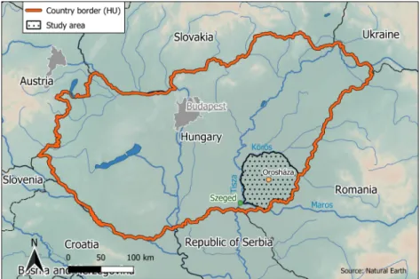
The study area is 5913 km²in the southeast of the Great Hungary Plain, enclosed by the Tisza, Körös and Maros rivers and the Hungarian–Romanian border (Figure1). The elevation is between 77 and 107 m (above Baltic mean sea level). The vulnerability to inland excess water of the area falls in the categories moderately endangered or strongly endangered [11].

approaches of combined monitoring of surface water with optical and radar data have appeared [34,35].

With the development of ESA’s Copernicus program, a large fleet of satellites has appeared that provides data for a large range of applications. The Sentinel-1 satellites have been among the first platforms in the program and provide data using an active remote sensing instrument. The data set is an improvement over earlier radar data sets because it provides continuous, near global data with a high temporal interval [36]. The Sentinel-2 satellites in the constellation are multispectral satellites with a high temporal interval as well. The combined use of Sentinel-1 and Sentinel-2 data has been studied for different applications, like land use/land cover classification [37–39] and wetlands mapping [40].

Although flood detection based on Sentinel-2 has been studied before [41,42], a fully automated approach based on a combination of Sentinel-1 and -2 to determine the extent of non-permanent shallow water bodies has not been published to the knowledge of the authors.

The aim of our research is to develop a methodology that is capable of continuously monitoring inland excess water over large areas to improve complex water management. Our research questions are (1) what combination of satellite data can be used for large-scale IEW mapping, (2) which methods can be fully automated to be able to create standardized, repeatable, weekly IEW maps and (3) what is the accuracy of the methodology? In 2017, a first attempt was made to combine passive and active satellite data to create regional scale inland excess water maps. Results of IEW detection based on the combined satellite data sources were promising but were still quite error prone [10]. Therefore, the algorithms were improved and fully automated. Here, we present a new workflow that is capable of fully automatic processing of freely available data of Sentinel-1A, Sentinel-1B, Sentinel-2A and Sentinel-2B into weekly inland excess water maps at regional or national scales. We also present validation of the results based on independent high-resolution satellite data and aerial photographs.

2. Materials and Methods 2.1. Study Area

The study area is 5913 km² in the southeast of the Great Hungary Plain, enclosed by the Tisza, Körös and Maros rivers and the Hungarian–Romanian border (Figure 1). The elevation is between 77 and 107 m (above Baltic mean sea level). The vulnerability to inland excess water of the area falls in the categories moderately endangered or strongly endangered [11].

Figure 1. Study area of inland excess water mapping.

The areas that are most vulnerable are southeast of the city of Orosháza, the low-lying plains in the west, the valley of the lower Tisza and the areas close to the Körös river. There is a close relation

Figure 1.Study area of inland excess water mapping.

(4)

The areas that are most vulnerable are southeast of the city of Orosháza, the low-lying plains in the west, the valley of the lower Tisza and the areas close to the Körös river. There is a close relation between these areas and the regularly flooded regions prior to the 19th century river regulations [15].

Due to the geomorphological characteristics of the Maros alluvial fan, IEW can also develop on the higher areas, which can cause significant damage at the border of the alluvial fan [2].

The development of inland excess water in the study area is favored by the fact that 84% of the soils are clayey, 50% of them have poor water absorption and unfavorable water management characteristics, and their upper, middle and lower layers are easily saturated. Eighty eight percent of the agricultural land is arable land, which is because more than 75% of the soils are fertile chernozem.

The build-up area ratio in the study area is 5%.

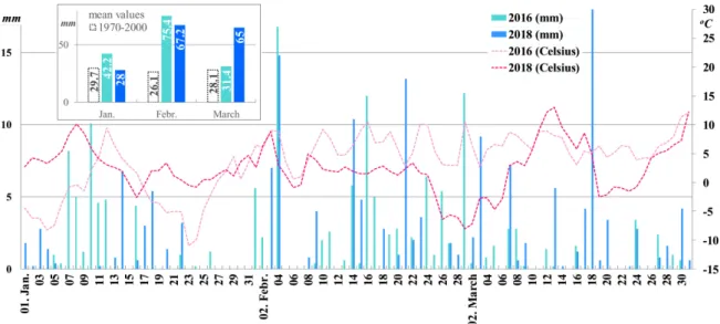
The development of IEW is closely, but not exclusively, related to the period with high precipitation in January, February and March. For this reason, our research period is focused on, respectively, March 2016 and March 2018 (Figure2). In 2016, during the period between January and March the precipitation was continuously above the 1971–2000 long-term average for that period, while in February it was even twice as high as normally. After the high precipitation period in the second half of February, between March 14–20, just before and during the satellite data acquisition, also quite a lot of rain fell. The temperature of 5–10^◦C was several degrees above the normal temperature in February and March, causing increased evaporation.

Sustainability 2020, 12, x FOR PEER REVIEW 4 of 21

between these areas and the regularly flooded regions prior to the 19th century river regulations [15].

Due to the geomorphological characteristics of the Maros alluvial fan, IEW can also develop on the higher areas, which can cause significant damage at the border of the alluvial fan [2].

The development of inland excess water in the study area is favored by the fact that 84% of the soils are clayey, 50% of them have poor water absorption and unfavorable water management characteristics, and their upper, middle and lower layers are easily saturated. Eighty eight percent of the agricultural land is arable land, which is because more than 75% of the soils are fertile chernozem.

The build-up area ratio in the study area is 5%.

The development of IEW is closely, but not exclusively, related to the period with high precipitation in January, February and March. For this reason, our research period is focused on, respectively, March 2016 and March 2018 (Figure 2). In 2016, during the period between January and March the precipitation was continuously above the 1971–2000 long-term average for that period, while in February it was even twice as high as normally. After the high precipitation period in the second half of February, between March 14–20, just before and during the satellite data acquisition, also quite a lot of rain fell. The temperature of 5–10 °C was several degrees above the normal temperature in February and March, causing increased evaporation.

Figure 2. Daily precipitation and temperature data on the study area between 01 January–31 March in 2016 and 2018 respectively and the deviation of the monthly precipitation amount from the 1971–

2000 climatic normal value based on a summation of the 5 closest meteorological stations (Hungarian Meteorological Service, OGIMET) (the colored days on the x-axis show the remote sensing data acquisition dates in 2016 and 2018).

In February 2016, everywhere on the Great Hungarian Plain inland excess water developed. In March, IEW in Hungary peaked at a maximum 82,427 ha [43]. The year 2016 can be considered a moderate IEW year in terms of total area covered by water.

In February, as well as in March 2018, the precipitation was twice as high as the national long- term average between 1971–2000 for those months. In fact, in the south part of the study area, the precipitation was already above the seasonal average in January. At the end of February, a cold period with precipitation started, which resulted in a considerable layer of snow. The warmer period in the middle of March caused the snow to melt and the soil to get saturated by melting water. Also, substantial rainfall fell during March, especially on the 18th. The satellite imagery from March 28, 29, 30 and 31 used in the study shows the development of IEW at the end of March. The total area covered by IEW in Hungary was 73,184 ha [44], slightly less than in 2016. This year should also be considered a moderate IEW year.

2.2. Data

Figure 2.Daily precipitation and temperature data on the study area between 01 January–31 March in 2016 and 2018 respectively and the deviation of the monthly precipitation amount from the 1971–2000 climatic normal value based on a summation of the 5 closest meteorological stations (Hungarian Meteorological Service, OGIMET) (the colored days on the x-axis show the remote sensing data acquisition dates in 2016 and 2018).

In February 2016, everywhere on the Great Hungarian Plain inland excess water developed.

In March, IEW in Hungary peaked at a maximum 82,427 ha [43]. The year 2016 can be considered a moderate IEW year in terms of total area covered by water.

In February, as well as in March 2018, the precipitation was twice as high as the national long-term average between 1971–2000 for those months. In fact, in the south part of the study area, the precipitation was already above the seasonal average in January. At the end of February, a cold period with precipitation started, which resulted in a considerable layer of snow. The warmer period in the middle of March caused the snow to melt and the soil to get saturated by melting water. Also, substantial rainfall fell during March, especially on the 18th. The satellite imagery from March 28, 29, 30 and 31 used in the study shows the development of IEW at the end of March. The total area covered

(5)

by IEW in Hungary was 73,184 ha [43], slightly less than in 2016. This year should also be considered a moderate IEW year.

2.2. Data

The presented inland excess water mapping workflow integrates different remote sensing datasets with auxiliary vector and raster data. The satellite images were obtained from the scientific data hub of the Copernicus Earth observation program of ESA [44].

2.2.1. Sentinel Satellite Data

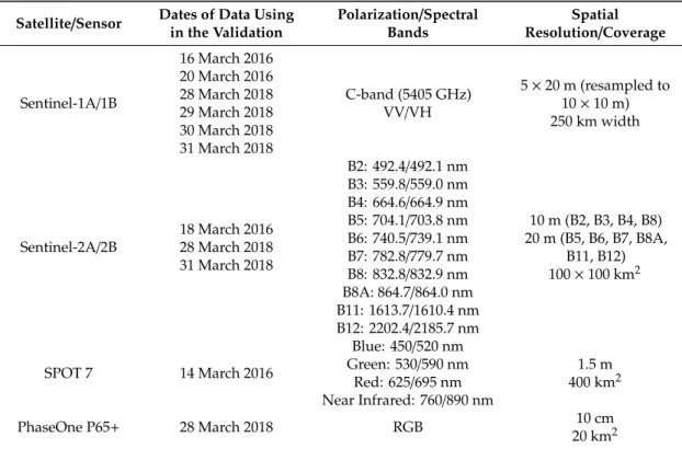
Sentinel-1 satellite constellation offers C-band radar data, day and night, and under all weather conditions. At the study area, the two satellites provide images about every third day in three descending and two ascending paths. The applied Interferometric Wide (IW) swath mode covers a 250 km wide area and has 5×20 m spatial resolution. Level 1 Ground Range Detected (GRD) products containing both Vertical–Vertical (VV) and Vertical–Horizontal (VH) polarizations were automatically downloaded for the selected time frame and preprocessed in several steps. For the validation of the research methodology, in total, 9 radar images were processed for 2016 and 21 for 2018 (Table1).

Table 1.Remotely sensed input data.

Satellite/Sensor Dates of Data Using in the Validation

Polarization/Spectral Bands

Spatial Resolution/Coverage

Sentinel-1A/1B

16 March 2016 20 March 2016 28 March 2018 29 March 2018 30 March 2018 31 March 2018

C-band (5405 GHz) VV/VH

5×20 m (resampled to 10×10 m) 250 km width

Sentinel-2A/2B 18 March 2016 28 March 2018 31 March 2018

B2: 492.4/492.1 nm B3: 559.8/559.0 nm B4: 664.6/664.9 nm B5: 704.1/703.8 nm B6: 740.5/739.1 nm B7: 782.8/779.7 nm B8: 832.8/832.9 nm B8A: 864.7/864.0 nm B11: 1613.7/1610.4 nm B12: 2202.4/2185.7 nm

10 m (B2, B3, B4, B8) 20 m (B5, B6, B7, B8A,

B11, B12) 100×100 km²

SPOT 7 14 March 2016

Blue: 450/520 nm Green: 530/590 nm

Red: 625/695 nm Near Infrared: 760/890 nm

1.5 m 400 km²

PhaseOne P65+ 28 March 2018 RGB 10 cm

20 km²

Sentinel-2 multispectral imaging satellites provide optical data with a five-day revisiting period (Table1). From the available 13 spectral bands, covering the spectra from the visible part through near infrared to short-wave infrared, only 10 bands with 10 and 20 m spatial resolution were used in the analysis. In the first validation period in 2016, only the Sentinel-2A satellite was in orbit and just the Level 1C (L1C) data product was available for download. In 2018, also data from Sentinel-2B, at Level 2A (L2A, Bottom-of-Atmosphere (BoA) reflectance values) was accessible. In the Sentinel-2 granule system, the study area is fully covered by four 100×100 km tiles: 34TDT, 34TDS, 34TET and 34TES.

Altogether, optical images from three different dates were processed in this research.

(6)

2.2.2. Validation Data

In the validation process, independent remote sensing data, acquired by satellite and aerial sensors, were used. In 2016, reference data of inland excess water patches was generated from a SPOT-7 image.

In 2018, an orthophoto was used to create the reference data set.

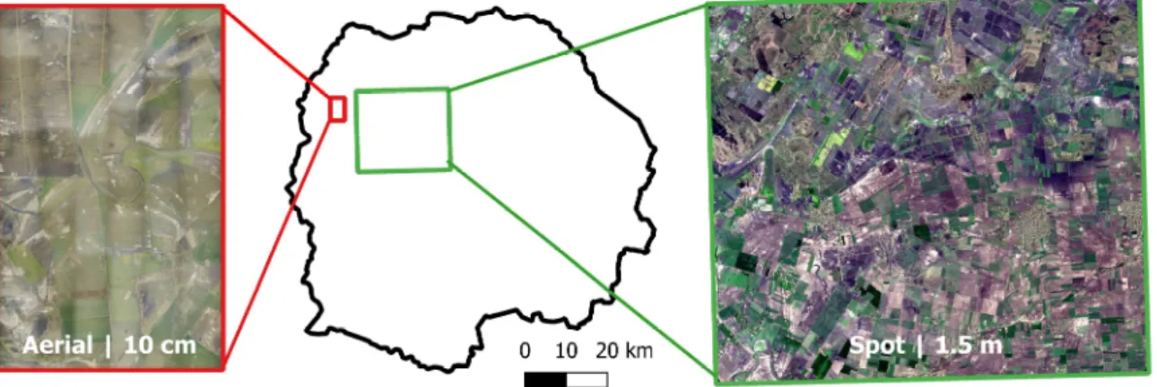
The acquisition date of the pan-sharpened SPOT-7 image was 14 March 2016. The spatial resolution of the orthorectified data was 1.5 m due to pan sharpening of the original 6 m multispectral bands. The image covered an area of 400 km²in the northwest part of the study area (Figure3).

In the validation process, independent remote sensing data, acquired by satellite and aerial sensors, were used. In 2016, reference data of inland excess water patches was generated from a SPOT-7 image. In 2018, an orthophoto was used to create the reference data set.

The acquisition date of the pan-sharpened SPOT-7 image was 14 March 2016. The spatial resolution of the orthorectified data was 1.5 m due to pan sharpening of the original 6 m multispectral bands. The image covered an area of 400 km² in the northwest part of the study area (Figure 3).

Figure 3. Validation sites in the study area.

Aerial photographs were taken on 28 March 2018 with a 60 MP RGB camera deployed on a Cessna 172 airplane. The generated orthophoto mosaic had 10 cm spatial resolution and covered an area of approximately 20 km² in the northwest of the study area.

2.2.3. Auxiliary Data

The satellite data-based algorithm requires multiple mask files to identify and evaluate inland excess water inundations. Permanent water bodies in the study area, like lakes and rivers, were extracted and stored in a training mask file (reference areas). Based on this mask, reference statistics were calculated that were used by the three algorithms of the workflow to identify pixels with water.

The mask was initially derived from vector maps stored in the hydro-geographic database of the General Directorate of Water Management. These maps were manually updated using very high resolution satellite images stored in Google Earth. Only open water was digitized, while avoiding vegetation along the shores and shadows. In total, 1400 ha of training pixels was extracted evenly spread over the study area.

The presented algorithm only assesses areas where temporary inundations can develop;

therefore, built-up areas, anthropogenic land cover like large roads, railroads and large buildings were excluded, using buffers of respectively 10 and 20 m. Also, permanent water bodies were not considered as IEW. This way only areas with nature, agriculture and forest were considered as potential IEW areas. Based on these criteria, areas were extracted from the National High Resolution Layer (nHRL) with a 10 m spatial resolution created by the Lechner Knowledge Center. Furthermore, large-scale vector maps stored in the hydro-geographic database of the General Directorate of Water Management were extracted and used to update the potential IEW areas. In this way, 12% of the study area was excluded for evaluation as IEW area.

2.3. Methodology

A large number of satellite images needs to be processed to be able to create the weekly inland excess water maps. This requires automation of the data processing workflow (Figure 4). For this purpose, a set of Python scripts was developed that combined standard libraries like gdal and numpy with arcpy for GIS operations. Two sets of scripts ran with a different interval. The daily set comprised downloading, preprocessing and processing data when new satellite images became

Figure 3.Validation sites in the study area.

Aerial photographs were taken on 28 March 2018 with a 60 MP RGB camera deployed on a Cessna 172 airplane. The generated orthophoto mosaic had 10 cm spatial resolution and covered an area of approximately 20 km²in the northwest of the study area.

2.2.3. Auxiliary Data

The satellite data-based algorithm requires multiple mask files to identify and evaluate inland excess water inundations. Permanent water bodies in the study area, like lakes and rivers, were extracted and stored in a training mask file (reference areas). Based on this mask, reference statistics were calculated that were used by the three algorithms of the workflow to identify pixels with water.

The mask was initially derived from vector maps stored in the hydro-geographic database of the General Directorate of Water Management. These maps were manually updated using very high resolution satellite images stored in Google Earth. Only open water was digitized, while avoiding vegetation along the shores and shadows. In total, 1400 ha of training pixels was extracted evenly spread over the study area.

The presented algorithm only assesses areas where temporary inundations can develop; therefore, built-up areas, anthropogenic land cover like large roads, railroads and large buildings were excluded, using buffers of respectively 10 and 20 m. Also, permanent water bodies were not considered as IEW. This way only areas with nature, agriculture and forest were considered as potential IEW areas.

Based on these criteria, areas were extracted from the National High Resolution Layer (nHRL) with a 10 m spatial resolution created by the Lechner Knowledge Center. Furthermore, large-scale vector maps stored in the hydro-geographic database of the General Directorate of Water Management were extracted and used to update the potential IEW areas. In this way, 12% of the study area was excluded for evaluation as IEW area.

2.3. Methodology

A large number of satellite images needs to be processed to be able to create the weekly inland excess water maps. This requires automation of the data processing workflow (Figure4). For this purpose, a set of Python scripts was developed that combined standard libraries like gdal and numpy

(7)

with arcpy for GIS operations. Two sets of scripts ran with a different interval. The daily set comprised downloading, preprocessing and processing data when new satellite images became available, while the second set ran on a weekly basis and integrated the daily results into the weekly map.

available, while the second set ran on a weekly basis and integrated the daily results into the weekly map.

Figure 4. Inland excess water detection workflow based on preprocessed Sentinel-1 and Sentinel-2 data. The elements with a green background indicate the optical data based Modified Normalized Difference Water Index (MNDWI) workflow, the yellow background indicates the optical data based Iterative Self-Organizing Data Analysis Technique (ISODATA) classification workflow and the blue background indicates the radar data-based workflow.

2.3.1. Downloading the Base Satellite Data

Sentinel-1 and -2 data can be downloaded free of charge from ESA’s Copernicus Open Access Hub. With the help of a Python script, the Wget program (www.gnu.org/software/wget) was called to search for relevant Sentinel images. A list with images was returned and processed to extract the image URLs. These URLs were fed to Wget, and the files were downloaded sequentially. If, due to overload of the ESA server or other reasons, the file was not downloaded correctly, the process was restarted automatically after a defined time interval. The script was restarted every day in the week

Figure 4. Inland excess water detection workflow based on preprocessed Sentinel-1 and Sentinel-2 data. The elements with a green background indicate the optical data based Modified Normalized Difference Water Index (MNDWI) workflow, the yellow background indicates the optical data based Iterative Self-Organizing Data Analysis Technique (ISODATA) classification workflow and the blue background indicates the radar data-based workflow.

2.3.1. Downloading the Base Satellite Data

Sentinel-1 and -2 data can be downloaded free of charge from ESA’s Copernicus Open Access Hub. With the help of a Python script, the Wget program (www.gnu.org/software/wget) was called to search for relevant Sentinel images. A list with images was returned and processed to extract the image URLs. These URLs were fed to Wget, and the files were downloaded sequentially. If, due to overload

(8)

of the ESA server or other reasons, the file was not downloaded correctly, the process was restarted automatically after a defined time interval. The script was restarted every day in the week that was processed because sometimes data only became available a few days later instead of immediately after acquisition.

2.3.2. Preprocessing

Sentinel-1 data were preprocessed using the ESA SNAP graph processing tool (gpt). With this command line interface, SNAP image processing functions can be accessed and automatically executed [45]. Each Sentinel-1 image was individually processed to generate a geometrically and radiometrically corrected sigma0 output. The images were transformed using Rangle Doppler Terrain Correction to UTM 10 × 10 m images that can be combined with the other data sets. After the preprocessing phase, an additional step was performed to reduce the effect of the incidence angle on the backscatter values, by normalizing every pixel in the preprocessed image using the local incidence angle.

Depending on the age of the Sentinel-2 data, the preprocessing workflow was slightly different because older data were only available in level 1C format. Level 1C data have to be transformed into level 2A using ESA’s Sen2Cor algorithm. Once the data were in level 2A format, selected spectral bands (Table1) were resampled and cloud masked using a custom ESA SNAP graph. Cloud and cloud shadow masks were generated from the level 2A scene classification layer. Sentinel-2 tiles slightly overlapped each other, which would cause overestimation of the IEW pixels if each tile would be processed separately. Therefore, single tiles were mosaiced into the original swath at each acquisition day. For the validation of the presented methodology, Sentinel-2 data in level 1C format were downloaded in 2016, while in 2018 the data were in level 2A format.

2.3.3. Processing Radar-Based Processing

The preprocessed Sentinel-1 images were filtered using a Refined Lee speckle filter to reduce noise.

Then, the backscatter values were converted to decibel (db) units for easier handling in the processing workflow. The radar processing workflow was based on the assumption that the radar response of water was considerably lower than the response of other pixels. The challenge is to find the maximum backscatter value of water [33,46]. To determine this value, training data were collected for both the VV and VH bands of an image. The training data consists of the statistics of the known water bodies as described in 2.2.3. For each band, the minimum, average and standard deviation were determined.

Based on these values, the upper and lower thresholds are calculated using an empirically determined method:

uthr_b =x+k∗σ (1)

lthr_b=x_min+ (₃^∗(x−x_min)_/5) ₍₂₎ where

bis, respectively, band VV or band VH;

uthrbis the upper threshold in db;

lthrbis the lower threshold in db;

xis the mean of the training samples in db;

σis the standard deviation of the training samples in db;

xminis the minimum of the training samples in db;

kis a user defined constant that can be adapted to specify the sensitivity of the algorithms to water, where a higher value results in more pixels to be identified as water. The value for k is empirically determined based on the inland excess water events in 2016 and 2018 described in the research. In the future, when more data are available for new IEW periods, the value for this constant can be fine-tuned.

(9)

Sometimes, due to speckle or artifacts, pixels with very low backscatter values occur in the images.

These pixels are excluded as water using the lower threshold. All pixels that are between the upper and lower thresholds in both bands are stored as water pixels:

water pixel=lthrb<xb<uthrb (3) wherexbis the value of an individual pixel.

In the rare case that the statistics of the training samples are beyond the normal range, the predetermined standard values are used for the lower and upper thresholds. These are band-specific (lthrVV=⁻40, uthrVV=⁻17,lthrVH =⁻50 anduthrVH =⁻23) because backscatter values for water are normally lower in the VH band. The predetermined standard values are a requirement for full automation of the algorithm. Their values are based on examining the values of water in the radar images and literature [27,30]. Ascending and descending orbits are processed using the same methods because each image is processed individually, meaning that every image has its own set of training statistics that is used for the extraction on the water pixels.

It was observed that in areas with sandy soils, the backscatter values were lower, resulting in overestimation of the number of water pixels. Therefore, an adaptation of the radar processing was applied to each sandy pixel in the image, and the upper threshold was reduced by 25%. This value was empirically calibrated. So far, its value could not be better determined from other research. The value can be adapted when more data become available from other IEW periods or other areas. Pixels defined as water in both bands are considered water pixels and are stored in the final map.

The final map is a binary map showing all water in the area, whether it is an inland excess water inundation or a permanent water body like a lake or a river.

Optical Data Based Classification

Open water surfaces are extracted from preprocessed Sentinel-2 optical data using two different approaches. The first one applies an automatic multispectral classification based on Iterative Self-Organizing Data Analysis Technique (ISODATA) clustering [47]. The mean values of the reference permanent water bodies (see Section2.2.3) are calculated for each Sentinel-2 band. These statistics are then compared to the statistics of the ISODATA output classes. The comparison is based on the nD similarity measurement of the spectral angle difference:

cos⁻¹







Pnb i=1tiri

Pnb

i=1t²_i1/2Pnb i=1r²_i1/2







(4)

where

nbis the number of selected Sentinel-2 bands;

tis the list of mean values of the selected Sentinel-2 bands in the examined ISODATA class;

ris the list of mean values of the selected Sentinel-2 bands in the training pixel group.

Natural breaks were identified among similarity values, which are ordered by increasing value.

The most similar ISODATA classes were normally located before the first break, and they were labeled as “water” classes. The method requires a sufficient number of training pixels, which is sometimes difficult to acquire due to cloud cover in the optical data. Therefore, a checking and verification step was implemented in the algorithm. In case of insufficient quantity of reference data (less than 30,000 training pixels), the Sentinel-2 classification was not performed. Furthermore, if the statistics were beyond the normal range, empirically defined values for the mean of each band were used for the classification. The classified raster was reclassified to a binary map, differentiating water and non-water pixels.

(10)

Optical Data Based Index Calculation and Thresholding

The Modified Normalized Difference Water Index (MNDWI) was developed by Xu [48] and is an enhanced version of the algorithm originally proposed by McFeeters [49]. It is calculated from the green and Shortwave-Infrared (SWIR) bands, and it is one of the most popular methods to extract water from multispectral satellite imagery. The index produces positive values for the water and negative values for built-up, soil and vegetation land cover:

MNDWI= ^ρ^green

−ρSWIR

ρgreen+ρSWIR (5)

where

ρgreenandρSWIRare the BoA reflectance of the green and SWIR bands.

The SWIR band (Sentinel-2, Band 11) originally had a spatial resolution of 20 m whilst the green band (Sentinel-2, Band 3) had a resolution of 10 m. To take full advantage of the 10 m information provided by the Sentinel-2 images, a 10 m spatial resolution MNDWI was produced through resampling the 20 m resolution band during the preprocessing phase.

Water bodies were mapped by a simple slicing algorithm using a suitable threshold value.

In general, the MNDWI value of a pixel larger than zero was considered as water. In practice, even though atmospherically corrected, multispectral images acquired at different regions and different times always have slightly different characteristics, thus the threshold needs to be empirically adjusted for each region and acquisition date using a multiplication factor:

MNDWIthreshold=MNDWImean−k∗MNDWIstd (6) where

MNDWImeanis the mean index value of the training samples;

MNDWI_stdis the standard deviation of the training samples;

kis a multiplication factor with a default value of 1.

If, due to cloud cover, the number of pixels with reference data is less than 30,000, or if the statistics are beyond the normal range, a standard value was used for the Sentinel-2 MNDWI segmentation threshold. Based on experiences of Du et al. [50], the ideal MNDWI threshold value is between 0.2–0.35. The result of the MNDWI segmentation process is a binary map, differentiating water from non-water pixels.

Integration

The binary maps produced by the three processing workflows covered different spatial areas and were from different dates during the week that was being processed. Data from different dates were aggregated into one weekly inland excess water map because data from single date do not provide a reliable result [10]. To integrate the data and to determine the reliability of the final weekly inland excess water map, all individual partial result maps were extended to the total study area. Pixels where no information was available on whether there was water were designated−100. Pixels can have a−100 value if they are clouds, shadows, outside the original image or for any other reason undetermined. The result is a large set of maps with three values: 0 (no water), 1 (water), and−100 (undetermined) covering the total study area. In the next step, a map was created storing the number of times that it was determined if in a pixel there was water or no water. In another map, for each pixel, it was determined how many times water was found. By dividing the second map by the first map, a frequency map was created specifying the relative number of times water was found in a pixel compared to the number of times data were available. If the relative frequency of water was above the manually specified threshold (e.g., 0.3 or 30%), the pixel was determined to be water. This map was

(11)

then filtered to delete separate water pixels surrounded by no water pixels and to fill up individual no water pixels surrounded by water pixels. In this way, more continuous inundations were generated.

In the final step, all known permanent water bodies were masked out based on the masked file (see Section2.2.3), and a binary raster inland excess water map was created. The raster map was vectorized, and using zonal statistics the amount of inland excess water per hectare was calculated for different administrative units.

2.3.4. Validation

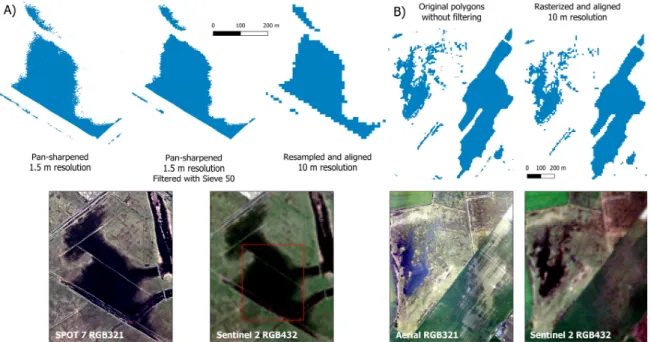
Validation data for the 2016 inland excess water period were derived from a pan-sharpened multispectral SPOT-7 image. Water surfaces were extracted using an automated clustering method (ISODATA with 60 classes), combined with manual selection of water classes. From the classified raster, gaps and separated water pixels smaller or equal to the mapping resolution (10×10 m) were removed using the Sieve method. Permanent water bodies, linear infrastructures, built-up areas and shadows were also removed. In the last step, the validation data were resampled and aligned to the processing grid of Sentinel-2 data (Figure5).

Validation data for the 2016 inland excess water period were derived from a pan-sharpened multispectral SPOT-7 image. Water surfaces were extracted using an automated clustering method (ISODATA with 60 classes), combined with manual selection of water classes. From the classified raster, gaps and separated water pixels smaller or equal to the mapping resolution (10 × 10 m) were removed using the Sieve method. Permanent water bodies, linear infrastructures, built-up areas and shadows were also removed. In the last step, the validation data were resampled and aligned to the processing grid of Sentinel-2 data (Figure 5).

Figure 5. Processing of validation data from SPOT-7 image (A) and from aerial survey (B). Both images show a small subsection of the validation areas.

The 2018 validation was based on an orthophoto mosaic covering an area of 20 km² in the northwest part of the study area. It was visually interpreted, and inland excess water patches were manually digitized. Polygons were filtered by deleting objects smaller than 100 m² and resampled and aligned to the processing grid (Figure 5). The rasterized validation datasets and the result inland excess water maps were compared using a cross-tabulation method. The producer’s and user’s accuracy and omission and commission error were calculated for the water and no water classes.

3. Results and Discussion

3.1. Maps and Statistics

Weekly inland excess water maps were created for the complete study area for the two inland excess water periods in 2016 and 2018 (Figure 6). Parameters were tweaked to adjust the sensitivity of the algorithm to water but to stay within realistic boundaries. Visual inspection of the results, overlaying the IEW maps on different color composites of the Sentinel-2 images, shows that the algorithm properly delineated IEW inundations. The largest inundations were detected in regions with clayey soils with unfavorable water management characteristics and on the former floodplains, delineating the former fluvial geomorphology like oxbows and river meanders. The border of the Maros alluvial fan was clearly shown on the 2018 result, in fact even on its higher areas IEW was detected.

Figure 5.Processing of validation data from SPOT-7 image (A) and from aerial survey (B). Both images show a small subsection of the validation areas.

The 2018 validation was based on an orthophoto mosaic covering an area of 20 km² in the northwest part of the study area. It was visually interpreted, and inland excess water patches were manually digitized. Polygons were filtered by deleting objects smaller than 100 m²and resampled and aligned to the processing grid (Figure5). The rasterized validation datasets and the result inland excess water maps were compared using a cross-tabulation method. The producer’s and user’s accuracy and omission and commission error were calculated for the water and no water classes.

3. Results and Discussion

3.1. Maps and Statistics

Weekly inland excess water maps were created for the complete study area for the two inland excess water periods in 2016 and 2018 (Figure6). Parameters were tweaked to adjust the sensitivity of the algorithm to water but to stay within realistic boundaries. Visual inspection of the results, overlaying the IEW maps on different color composites of the Sentinel-2 images, shows that the

(12)

algorithm properly delineated IEW inundations. The largest inundations were detected in regions with clayey soils with unfavorable water management characteristics and on the former floodplains, delineating the former fluvial geomorphology like oxbows and river meanders. The border of the Maros alluvial fan was clearly shown on the 2018 result, in fact even on its higher areas IEW was detected.Sustainability 2020, 12, x FOR PEER REVIEW 12 of 21

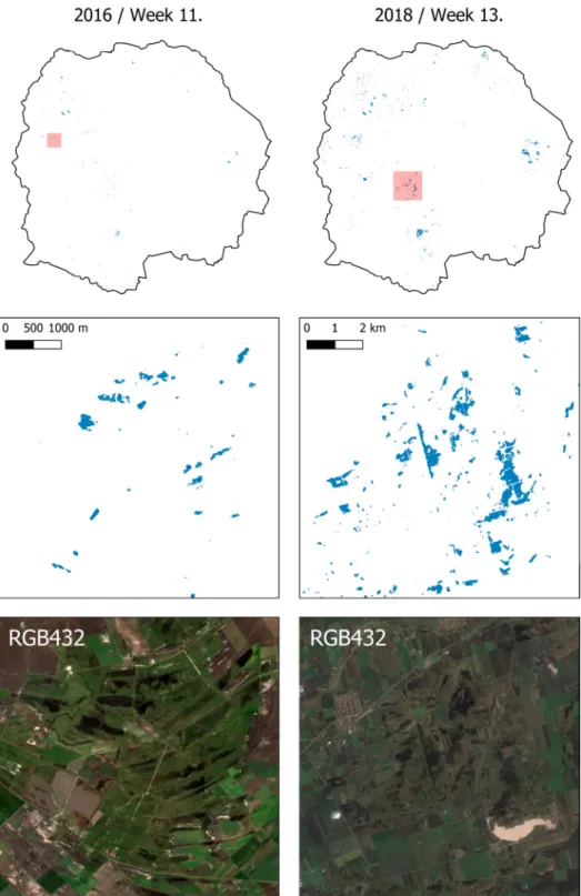
Figure 6. Detected inland excess water on the total study area (top) and on subareas (middle) in 11th week of 2016 (left) and 13th week of 2018 (right) and natural color composites of the input optical data (bottom).

During the moderate IEW period of 2016, the presented algorithm detected a little over 600 ha of IEW mainly in the northwest and east parts of the total study area. More than half of the detected IEW polygons were small, in this research not larger than 3 pixels (=< 300 m²). Often in pixel-based classifications, these pixels are automatically attached to the statistically nearest bigger class. In the presented algorithm, this procedure did not happen because the contrast between water surfaces and dry surfaces is usually quite big, and these small patches are often located close to each other or part of a larger patch, together defining a larger flood area in the IEW map. In 2016, 72% of the IEW patches

Figure 6.Detected inland excess water on the total study area (top) and on subareas (middle) in 11th week of 2016 (left) and 13th week of 2018 (right) and natural color composites of the input optical data (bottom).

(13)

During the moderate IEW period of 2016, the presented algorithm detected a little over 600 ha of IEW mainly in the northwest and east parts of the total study area. More than half of the detected IEW polygons were small, in this research not larger than 3 pixels (=<300 m²). Often in pixel-based classifications, these pixels are automatically attached to the statistically nearest bigger class. In the presented algorithm, this procedure did not happen because the contrast between water surfaces and dry surfaces is usually quite big, and these small patches are often located close to each other or part of a larger patch, together defining a larger flood area in the IEW map. In 2016, 72% of the IEW patches consisted of large, minimum 1 ha inundations, the largest patch was even larger than 25 ha. The results show that over half of the IEW inundations occurred in agricultural areas, to a large extent arable land, which has a large effect on the agricultural production. A further one-third of the IEW patches were located on natural grassland.

In 2018, almost four times as much inland excess water was detected (3082 ha) as in 2016, and also the spatial distribution of the patches was more spread out than in the earlier research period. In fact, the floods increased everywhere except on the higher regions of the central and south-eastern parts of the study area. The complexity of the issue of inland excess water formation and the importance of high-resolution monitoring was also demonstrated by the fact that in 2016, there were small IEW patches that were not inundated in 2018 (e.g., the arable land northwest of Orosháza).

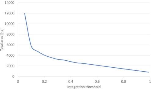
For 2018, it was tested how the algorithm responded to different settings of the integration parameter (Figure7). Thresholds for 0.05 to 1 were specified with an increment of 0.05. The final setting that was used for the calculations of inland excess water in 2016 and 2018 was 0.30. It was determined that lower settings resulted in a large amount of cloud and shadow misclassification, and higher settings reduced the amount of detected water too much.

consisted of large, minimum 1 ha inundations, the largest patch was even larger than 25 ha. The results show that over half of the IEW inundations occurred in agricultural areas, to a large extent arable land, which has a large effect on the agricultural production. A further one-third of the IEW patches were located on natural grassland.

In 2018, almost four times as much inland excess water was detected (3082 ha) as in 2016, and also the spatial distribution of the patches was more spread out than in the earlier research period. In fact, the floods increased everywhere except on the higher regions of the central and south-eastern parts of the study area. The complexity of the issue of inland excess water formation and the importance of high-resolution monitoring was also demonstrated by the fact that in 2016, there were small IEW patches that were not inundated in 2018 (e.g., the arable land northwest of Orosháza).

For 2018, it was tested how the algorithm responded to different settings of the integration parameter (Figure 7). Thresholds for 0.05 to 1 were specified with an increment of 0.05. The final setting that was used for the calculations of inland excess water in 2016 and 2018 was 0.30. It was determined that lower settings resulted in a large amount of cloud and shadow misclassification, and higher settings reduced the amount of detected water too much.

Figure 7. Relationship between the setting of the integration threshold and the total area of inland excess water in hectares in 2018.

It should be mentioned that the number of available input images in 2018 was much larger than that in 2016; therefore, the chance to detect water was also larger. This issue only occurred in the earlier years of Sentinel data acquisition when fewer satellites were in orbit. In both years, the large and often deeper inundations that were part of non-permanent wetlands (in the south center and east) were detected almost perfectly. There was also a difference in land use at the inundation between the two years under study. In 2018, the majority of inland excess water inundations affected natural grasslands, and in agricultural land the proportion of meadow pastures (21%) was higher than that of arable land (15%), while in 2016 the inundation mostly occurred on arable lands (34%).

More than 83% of the detected inundations were due to patches larger than 1 ha, but in 2016 there were many patches that consisted of one large polygon: several 40–60 ha patches were detected, while the largest had an area of 331 ha.

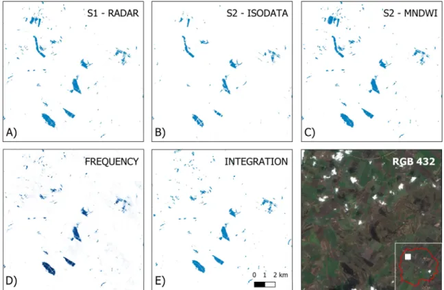
Figure 8 shows a set of submaps of the detection results of 2018. At the top, it can be seen that the three detection workflows identified similar patterns of water, but there were some differences.

The MNDWI-based water maps showed the most water, while the ISODATA-based map was the least sensitive to water in this area. The frequency map showed for each pixel in how many source images inland excess water was detected. It can be clearly seen that deep waterbodies were detected most of the time, while more shallow water at the border of the deep IEW patches was detected less often. These areas form the fuzzy boundary between water, saturated soil and dry land. The

Figure 7.Relationship between the setting of the integration threshold and the total area of inland excess water in hectares in 2018.

It should be mentioned that the number of available input images in 2018 was much larger than that in 2016; therefore, the chance to detect water was also larger. This issue only occurred in the earlier years of Sentinel data acquisition when fewer satellites were in orbit. In both years, the large and often deeper inundations that were part of non-permanent wetlands (in the south center and east) were detected almost perfectly. There was also a difference in land use at the inundation between the two years under study. In 2018, the majority of inland excess water inundations affected natural grasslands, and in agricultural land the proportion of meadow pastures (21%) was higher than that of arable land (15%), while in 2016 the inundation mostly occurred on arable lands (34%). More than 83% of the detected inundations were due to patches larger than 1 ha, but in 2016 there were many patches that

(14)

consisted of one large polygon: several 40–60 ha patches were detected, while the largest had an area of 331 ha.

Figure8shows a set of submaps of the detection results of 2018. At the top, it can be seen that the three detection workflows identified similar patterns of water, but there were some differences.

The MNDWI-based water maps showed the most water, while the ISODATA-based map was the least sensitive to water in this area. The frequency map showed for each pixel in how many source images inland excess water was detected. It can be clearly seen that deep waterbodies were detected most of the time, while more shallow water at the border of the deep IEW patches was detected less often.

These areas form the fuzzy boundary between water, saturated soil and dry land. The integration stored water pixels that were detected more often than the relative frequency threshold. Often cloud and cloud shadows disturb the IEW detection, as can be seen on the natural color composite. The algorithm takes this into account by masking the clouds and shadows in the optical data and ignoring these pixels in the relative frequency calculation. The cloud/shadow masking prevents the algorithm to derive IEW from the optical data, but since radar images are not influenced by atmospheric disturbance, these areas are evaluated for water by the active satellite data based workflow.

integration stored water pixels that were detected more often than the relative frequency threshold.

Often cloud and cloud shadows disturb the IEW detection, as can be seen on the natural color composite. The algorithm takes this into account by masking the clouds and shadows in the optical data and ignoring these pixels in the relative frequency calculation. The cloud/shadow masking prevents the algorithm to derive IEW from the optical data, but since radar images are not influenced by atmospheric disturbance, these areas are evaluated for water by the active satellite data based workflow.

Figure 8. Sub-results (A, B, C), frequency of water detection (D) and the integrated final inland excess water map (E) on a selected area during the 13th week of 2018.

Figure 9 shows the differences in IEW area between the three detection methods and the total area of detected inland excess water in the integration result for the same sub-area as used in Figure 8. In the sub-area, the results for the optical data based workflows contained smaller IEW areas due to the clearly identifiable clouds and shadows in the area. At those locations, pixels were not evaluated by the ISODATA and MNDWI algorithms because they were masked out in the preprocessing phase before the algorithms were run, based on the cloud mask incorporated with the Sentinel-2 level 2 data set. The radar-based result contained IEW pixels in cloud/shadow areas because the atmospheric disturbances did not influence the active remote sensing data.

Figure 8.Sub-results (A–C), frequency of water detection (D) and the integrated final inland excess water map (E) on a selected area during the 13th week of 2018.

Figure9shows the differences in IEW area between the three detection methods and the total area of detected inland excess water in the integration result for the same sub-area as used in Figure8.

In the sub-area, the results for the optical data based workflows contained smaller IEW areas due to the clearly identifiable clouds and shadows in the area. At those locations, pixels were not evaluated by the ISODATA and MNDWI algorithms because they were masked out in the preprocessing phase before the algorithms were run, based on the cloud mask incorporated with the Sentinel-2 level 2 data set. The radar-based result contained IEW pixels in cloud/shadow areas because the atmospheric disturbances did not influence the active remote sensing data.

(15)

Sustainability2020,12, 2854 15 of 21

integration stored water pixels that were detected more often than the relative frequency threshold.

Often cloud and cloud shadows disturb the IEW detection, as can be seen on the natural color composite. The algorithm takes this into account by masking the clouds and shadows in the optical data and ignoring these pixels in the relative frequency calculation. The cloud/shadow masking prevents the algorithm to derive IEW from the optical data, but since radar images are not influenced by atmospheric disturbance, these areas are evaluated for water by the active satellite data based workflow.

Figure 8. Sub-results (A, B, C), frequency of water detection (D) and the integrated final inland excess water map (E) on a selected area during the 13th week of 2018.

Figure 9 shows the differences in IEW area between the three detection methods and the total area of detected inland excess water in the integration result for the same sub-area as used in Figure 8. In the sub-area, the results for the optical data based workflows contained smaller IEW areas due to the clearly identifiable clouds and shadows in the area. At those locations, pixels were not evaluated by the ISODATA and MNDWI algorithms because they were masked out in the preprocessing phase before the algorithms were run, based on the cloud mask incorporated with the Sentinel-2 level 2 data set. The radar-based result contained IEW pixels in cloud/shadow areas because the atmospheric disturbances did not influence the active remote sensing data.

Figure 9.Distribution of detected inland excess water (IEW) by algorithm for a selected area in 2018.

Figure10shows the distribution of inland excess water per algorithm for the whole study area.

Here, the misclassifying of shadow as water by the optical data based ISODATA is clearly shown.

In areas with cloud shadows that were not masked out by ESA’s Sen2Cor cloud/shadow detection algorithm, the ISODATA classifier mixed up shadow and water. The MNDWI algorithm is also based on optical data, but it is not sensitive to this misclassification. The integration result was not influenced by the errors due to shadows because these only occurred in one sub-result and, therefore, do not meet the integration threshold to be incorporated in the final result.

Figure 9. Distribution of detected inland excess water (IEW) by algorithm for a selected area in 2018.

Figure 10 shows the distribution of inland excess water per algorithm for the whole study area.

Here, the misclassifying of shadow as water by the optical data based ISODATA is clearly shown. In areas with cloud shadows that were not masked out by ESA’s Sen2Cor cloud/shadow detection algorithm, the ISODATA classifier mixed up shadow and water. The MNDWI algorithm is also based on optical data, but it is not sensitive to this misclassification. The integration result was not influenced by the errors due to shadows because these only occurred in one sub-result and, therefore, do not meet the integration threshold to be incorporated in the final result.

Figure 10. Distribution of detected IEW by algorithm for the total study area in 2018.

Maps of aggregated values for the absolute and relative number of hectares of inundations were generated per administrative IEW defense areas (Figure 11). They support operative water management planning by the local Water Directorates, and they can help to estimate the required pumping capacity and expected duration of the floods. The aggregated inundation maps for all IEW defense areas can be combined to a country-wide IEW preparedness map that is used for the national water management program. The local amount of inundation can also help to identify areas for storage of IEW, like reservoirs or permanent wetlands for use of water in later dry periods, this way supporting sustainable water management.

Figure 11. Aggregated maps of absolute (left) and relative (right) areas of inundations per administrative inland excess water defense area in the 13th week of 2018.

3.2. Validation

The results of the IEW detection algorithm in 2016 were validated with a SPOT 7 image. A subsection of the area can be seen in Figure 12. Visual inspection shows that the darker colors in the SPOT natural color composite were similar in the Sentinel-2 color composite. Inland excess water was

Figure 10.Distribution of detected IEW by algorithm for the total study area in 2018.

Maps of aggregated values for the absolute and relative number of hectares of inundations were generated per administrative IEW defense areas (Figure11). They support operative water management planning by the local Water Directorates, and they can help to estimate the required pumping capacity and expected duration of the floods. The aggregated inundation maps for all IEW defense areas can be combined to a country-wide IEW preparedness map that is used for the national water management program. The local amount of inundation can also help to identify areas for storage of IEW, like reservoirs or permanent wetlands for use of water in later dry periods, this way supporting sustainable water management.

3.2. Validation

The results of the IEW detection algorithm in 2016 were validated with a SPOT 7 image.

A subsection of the area can be seen in Figure12. Visual inspection shows that the darker colors in the SPOT natural color composite were similar in the Sentinel-2 color composite. Inland excess water was mainly detected in the deepest parts of the inundations (true positive, green in the central map).

(16)

Sustainability2020,12, 2854 16 of 21

Many pixels along the border of the inundations were not designated as water by the algorithm (false negative). Rarely pixels were wrongly designated as water (false positive).

Figure 9. Distribution of detected inland excess water (IEW) by algorithm for a selected area in 2018.

Figure 10 shows the distribution of inland excess water per algorithm for the whole study area.

Here, the misclassifying of shadow as water by the optical data based ISODATA is clearly shown. In areas with cloud shadows that were not masked out by ESA’s Sen2Cor cloud/shadow detection algorithm, the ISODATA classifier mixed up shadow and water. The MNDWI algorithm is also based on optical data, but it is not sensitive to this misclassification. The integration result was not influenced by the errors due to shadows because these only occurred in one sub-result and, therefore, do not meet the integration threshold to be incorporated in the final result.

Figure 10. Distribution of detected IEW by algorithm for the total study area in 2018.

Maps of aggregated values for the absolute and relative number of hectares of inundations were generated per administrative IEW defense areas (Figure 11). They support operative water management planning by the local Water Directorates, and they can help to estimate the required pumping capacity and expected duration of the floods. The aggregated inundation maps for all IEW defense areas can be combined to a country-wide IEW preparedness map that is used for the national water management program. The local amount of inundation can also help to identify areas for storage of IEW, like reservoirs or permanent wetlands for use of water in later dry periods, this way supporting sustainable water management.

Figure 11. Aggregated maps of absolute (left) and relative (right) areas of inundations per administrative inland excess water defense area in the 13th week of 2018.

3.2. Validation

The results of the IEW detection algorithm in 2016 were validated with a SPOT 7 image. A subsection of the area can be seen in Figure 12. Visual inspection shows that the darker colors in the SPOT natural color composite were similar in the Sentinel-2 color composite. Inland excess water was

Figure 11.Aggregated maps of absolute (left) and relative (right) areas of inundations per administrative inland excess water defense area in the 13th week of 2018.

mainly detected in the deepest parts of the inundations (true positive, green in the central map). Many pixels along the border of the inundations were not designated as water by the algorithm (false negative). Rarely pixels were wrongly designated as water (false positive).

Figure 12. Results of the cross-validation on a selected area in 2016 (A—input Sentinel-2 data, B—

result assessment, C—validation of SPOT 7 data).

The quantification of the validation was based on a pixel-by-pixel comparison between the SPOT image and the algorithm result and shows that the overall accuracy was high, but Cohen’s kappa was low due to a very high omission error (Table 2). This is due to the fact that if one IEW patch was missed in the classification, a large number of pixels were misclassified and added to the omission error. Also, the classification is unbalanced due to the high number of “no water” compared to

“water” pixels.

Table 2. Accuracy assessment on the validation site in 2016. The color of the cells refers to the colors in Figure 12.

Reference

# pixels no water water Total Producer's Acc.

Omission error

User's Acc.

Commission error

Detected

no water 4,454,908 7807 4,462,715 99.92 0.08 99.83 0.17

water 3494 4513 8007 36.63 63.37 56.36 43.64

no data

(cloud) 118 0 118 Overall Acc. 99.74 Kappa 0.44

Total 4,458,520 12,320 4,470,840

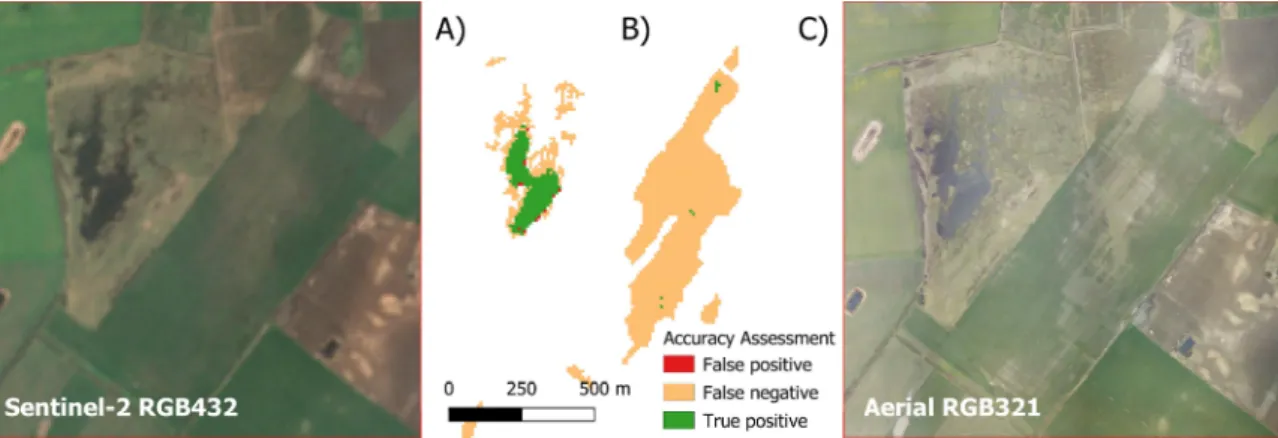
The IEW inundations delineated for the 2018 period were validated using the high-resolution orthophoto. From the orthophoto mosaic, 849 inland excess water patches covering 147.5 ha were digitized; however, the presented algorithm only delineated 52 polygons (8.9 ha). As can be seen in Figure 13, large inundations that were digitized on the aerial photograph can hardly be seen on the Sentinel-2 image and were also omitted by the algorithm. Like in 2016, the deep/dark water patches were delineated almost perfectly.

Figure 12.Results of the cross-validation on a selected area in 2016 (A—input Sentinel-2 data,B—result assessment,C—validation of SPOT 7 data).

The quantification of the validation was based on a pixel-by-pixel comparison between the SPOT image and the algorithm result and shows that the overall accuracy was high, but Cohen’s kappa was low due to a very high omission error (Table2). This is due to the fact that if one IEW patch was missed in the classification, a large number of pixels were misclassified and added to the omission error. Also, the classification is unbalanced due to the high number of “no water” compared to “water” pixels.

Table 2.Accuracy assessment on the validation site in 2016. The color of the cells refers to the colors in Figure12.

Reference

# Pixels No Water Water Total Producer’s Acc.

Omission Error

User’s Acc.

Commission Error