Article
Sentinel-1-Imagery-Based High-Resolution Water Cover Detection on Wetlands, Aided by Google Earth Engine
András Gulácsi and Ferenc Kovács *
Department of Physical Geography and Geoinformatics, University of Szeged, 6722 Szeged, Hungary;
h049952@stud.u-szeged.hu
* Correspondence: kovacsf@geo.u-szeged.hu; Tel.:+36-62-546-485
Received: 30 March 2020; Accepted: 14 May 2020; Published: 18 May 2020 Abstract: Saline wetlands experience large temporal fluctuations in water supply during the year and are recharged only or mainly through precipitation, meaning they are vulnerable to climate-change-induced aridification. Most passive satellite sensors are unsuitable for continuous wetland monitoring due to cloud cover and their relatively low temporal resolution. However, active satellite sensors such as the C-band synthetic aperture radar of Sentinel-1 satellites offer free, cloud-independent data. We examined surface water cover changes from October 2014 to November 2018 in the strictly protected area (13,000 ha) of the Upper-Kiskunság Alkaline Lakes region in the Danube–Tisza Interfluve in Hungary, with the aim of helping with nature protection planning.
Changes and sensitivity can be defined based on the knowledge of variability. We developed a method for water cover detection based on automatic classification, applying the so-called WEKA K-Means clustering algorithm. For satellite data processing and analysis, we used the Google Earth Engine cloud processing platform. In terms of validation, we compared our results with the multispectral Modified Normalized Difference Water Index (MNDWI) derived from Landsat 8 and Sentinel-2 top-of-atmosphere reflectance images using a threshold-based binary classifier (receiver operator characteristics) for the MNDWI data. Using two completely distinct methods operating in distinct wavelength ranges, we obtained adequately matching results, with Spearman’s correlation coefficients (ρ) ranging from 0.54 to 0.80.
Keywords: Sentinel-1; synthetic aperture radar; Google Earth Engine; wetlands; surface water cover;
cluster analysis
1. Introduction
Climate change could have a huge impact on the saline lake and wetland ecosystems of the Carpathian Basin, which present an ideal habitat for numerous protected species and are managed by national parks under the jurisdiction of certain laws and international agreements. Hungary currently has 29 sites designated as Wetlands of International Importance (Ramsar Sites), with a total surface area of 260,668 ha [1].
The wetlands of the Danube–Tisza Interfluve in Hungary are particularly vulnerable to changes in water availability because they are refilled only through precipitation. This is highlighted by the results of climate modelling projects that go beyond the current significant warming, increasing both drought frequency and drought severity [2,3].
In addition to the changes in the annual distribution of precipitation, the springtime reduction in precipitation and the increased evapotranspiration due to the increase in regional average temperatures and more frequent drought periods have negative implications in terms of the water balance of
Remote Sens.2020,12, 1614; doi:10.3390/rs12101614 www.mdpi.com/journal/remotesensing
wetlands, especially in the summer periods [4,5]. We can only define the changes in the water levels if we know the level of variability on the wetland surface areas, which are generally full of water in spring and totally dry in summer [6]. In view of this, further techniques are required for the study of wetland areas. With the use of SAR data, remote sensing may constitute an important additional information source for wetland inventory and management [7].
The aim of this study was to develop a method to obtain detailed snapshots of the current surface water cover conditions of wetlands using C-band synthetic aperture radar (C-SAR) data from the European Space Agency’s Sentinel-1 near-polar orbiting satellites for operative, continuous monitoring [8]. This will give us much greater insight into water cover dynamics, with the attendant results allowing us to monitor weather- or climate-change-related changes, which will provide us with important information for planning effective measures to protect the wetlands. We used Sentinel-1 images acquired in interferometric wide-swath mode, which presents an acquisition in a 250-km-wide track. The geometric resolution is 20 m×22 m, which was resampled to 10 m. The radar images are created in VH and VV polarization bands above the land, with a WGS84 projection. The revisiting time is six days with both satellites operating [8]. We used level-1 ground range detected (GRD) data for the analysis, taking images to analyze the surface water cover changes from October 2014 to November 2018. Before the second half of 2014, no radar data were freely available. Unfortunately, passive, multispectral satellite sensors are unsuitable for operative monitoring due to atmospheric disturbances (such as cloud cover and shadow, or aerosol gases). However, C-SAR provides clear images during the often-cloudy springtime, which is of great importance, because this period is one of the main water recharge periods for wetlands.
Radar data processing involves a great deal of time-consuming computation due to the numerous data processing steps involved [9,10]. The IT field of cloud computing emerged in early 2010 in response to the need for processing the huge amounts of digital data (so-called Big Data) continuously produced every second throughout the world [11,12]. Various cloud processing services have been made available via the internet, with the data processing software and the data itself stored centrally on large server farms or “internet clouds”. The user can access these through client-side applications and application program interfaces (APIs).
Google Earth Engine (GEE) is one such cloud processing platform, one that emerged to: (i) speed up satellite data processing, (ii) upscale it to a planetary scale, and (iii) serve scientists across the globe to ensure that environmental monitoring is more effective [13,14]. GEE provides a JavaScript API and a Python API for accessing the data and the scientific algorithms. The JavaScript API can be used in a web-based integrated development environment, the Earth Engine Code Editor, whereas the Python API requires an additional installation. We used JavaScript for the current study.
2. Materials and Methods
2.1. Study Area
According to the Köppen–Geiger climate classification system, Hungary has a humid continental climate with warm summers (subtype Dfb), and a large area of the country can experience hot summers (subtype Dfa) [15]. Our study area was the strictly protected area (13,000 ha) of the Upper-Kiskunság Alkaline Lakes region that encompasses a number of relatively large ”white saline lakes” (called ”szék”
in regional Hungarian) (Figure1), which are located on the Quaternary flood plain of the Danube and are bounded from the east by the middle, higher-elevated “sandland” part of the Danube–Tisza Interfluve landscape in the Great Hungarian Plain. Based on investigations over 130 years, Upper-Kiskunság Alkaline Lakes have been severely hit by droughts in the past decades. Concerning the optimistic and pessimistic scenarios, 5.6% and 33.5% of the study area will be affected negatively by water management strategies and precipitation changes, respectively [16].
Over the past 30 years, the mean temperature in the Danube–Tisza Interfluve has increased by 1.2◦C–1.5◦C, with climate models predicting that by 2050, the temperature will be between 1.4◦C
and 3.7◦C higher compared with the 1960–1990 reference period [3,17]. In terms of precipitation values, from 1901 only the 17% decrease in the spring can be considered as significant, whereas due to a number of rainy years (e.g., 2005, 2010), the last decade has experienced an increase. The average precipitation amount in the study area is, based on Kecskemét station’s long-term average (1930–2018), approximately 523 mm/year, with the period between 2014 and 2018 particularly significant because every year had an above-average level (2014 had the highest with 704 mm, and 2015 had the lowest with 532 mm) (Figure2). The seasonal amount was lowest in the summer (from April to September) of 2015 and in the winter (from October to March) of 2016/2017. The significant increase in temperature has led to an increased water demand in this region. The co-occurrence of above-average temperatures and below-average precipitation over the last two decades has largely characterized the spring periods [18].
Between 1995 and 2017, only eight years can be considered drought free.
Figure 1.The study area was the Upper-Kiskunság Alkaline Lakes (lake is called “szék” in regional Hungarian) (background image: Sentinel-1 2014–2018 composite; RGB: VH/VV/VV).
2.2. Surface Water Detection Using Sentinel-1 C-SAR
Although active radar imaging is unaffected by clouds, it is not completely weather-independent because it is affected by wind roughening effects. Wind shear creates waves on the waters, which increase the water surface roughness, resulting in higher radar backscatter at the radar antenna [19].
Water surfaces are generally smooth and are characterized by very low radar backscatter, but this is affected by wind roughening effects that result in the “erasing” of some water features on radar imagery.
The detection of surface waters is based on the difference in roughness between water-covered areas and other types of land cover. The higher the backscatter, the brighter the feature looks on the image and vice versa. As noted above, water features have very low roughness, and thus very low backscatter,
meaning they appear as very dark features that contrast strongly with their surroundings. In the study, we defined water as open water features regardless of their water depth. The ”white saline lakes” and other water surfaces in the study area are so shallow, generally between 20–50 cm, that the coastal and open water parts cannot be separated based on the water depth. The very high dissolved salt concentrations prevent the expansion of vegetation in these saline waters [20].
Figure 2.Precipitation amount and three-month precipitation ratio from 2014 to 2018 at the Kecskemét station: the ratio presents the normalization of the sum of one month’s precipitation and that of the two preceding months to the sum of the normal value (1971–2000) of this three-month amount of precipitation; the value 1 denotes the average data (data: Hungarian Meteorological Service).
Thresholding techniques on SAR images for surface water mapping are extensively used because of their efficiency and effectiveness. However, the accuracy of water separation from land is significantly affected by wind-induced roughening effects, poor image quality (speckle noise), and incidence angle variance, so the threshold needs to be modified on a scene per scene basis [21–27]. According to Manjusree el al. [21], at a near range to far range,−8 to−12 dB,−15 to−24 dB, and−6 to−15 dB can be used as optimum ranges for the classification of flood water in HH, HV, and VV polarizations. On the basis of our prior experience, surface water cover is characterized by backscatter values of around
−17–−18 dB or lower for the VV polarization band. Sokol et al. [28] found that a large decrease in backscatter occurs as the incidence angles increase, and backscatter values from Radarsat beam modes S1 to S7 (20–49◦) correspond to an average difference of 7 decibels. For Sentinel-1 IW modes (IW1 to IW3), the incidence angle range is similar: 29–46◦[29]. Shallow incidence angles (30–50◦) are preferred to maximize the contrast between land and water [30].
In the case of herbaceous wetlands (such as the study area), C-band SAR (frequency: 5 GHz;
wavelength: 5 cm) is more suitable for inundation detection, and lower frequencies (P-band, L-band) can be used for inundation detection with forest-covered or wooden wetlands [31–33]. Co-polarized (e.g., the same transmitted and received polarizations) polarization radar data (HH, VV) are more suitable for water cover detection; the most appropriate are HH co-polarized data, whereas VV polarizations are an adequate choice [34,35]. However, according to Brisco [30], VV polarization highlights surface roughness effects through the interaction of the capillary waves and the vertical polarization and is the least favored polarization to use. In addition, it is important to note that cross-polarized polarizations contain a great deal of useful information in terms of land cover mapping [36]. The backscatter of flood water in HV and VH is the same, and both HV and VH polarizations are adequate for the mapping of flood water [21].
2.3. Processing Data Using GEE
GEE already contains preprocessed Sentinel-1 radar imagery in its database. To derive the backscatter coefficient (in dB) for each pixel, the following preprocessing steps were performed via Google, based on the algorithms implemented by the Sentinel-1 Toolbox software [37,38]:
1. Applied orbit files.
2. GRD border noise removal.
3. Thermal noise removal (as of 12 January 2018).
4. Radiometric calibration (calculation of sigma naught values,σ0).
5. Terrain correction (orthorectification).
It is important to note that although the geometry of the backscatter estimate was corrected in GRD products, the radiometry of the resulting image remained an ellipsoid model based onσ0[39].
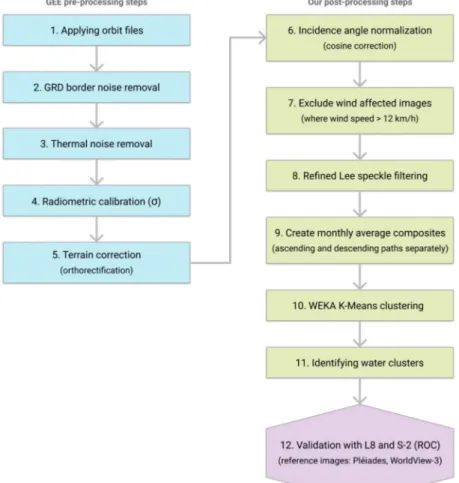
The remaining processing steps were performed using GEE (Figure3). The first and most critical step involved normalizing the backscatter coefficients because they are also dependent on the incidence angle. That is, the backscatter values of a specific area with a small incidence angle return higher backscatter values than the data of the same area acquired with a higher incidence angle. Moreover, incidence-angle-induced variations can also occur within a sensor using different acquisition geometries or different tracks or orbits. For Sentinel-1 time-series data, backscatter normalization is vital [40].
A technique that is widely used for this task is the cosine correction method [41,42], which was used in this study in terms of the ellipsoidal incidence angles.
Figure 3.Flowchart of the data processing steps applied to Sentinel-1 data. The pre-processing steps (1–5) had already been performed by Google. Steps 6–11 were done in the Google Earth Engine (GEE) application.
For the validation process, the fully processed data were downloaded (code available in AppendixA).
Small [39] argues that such angle-based normalizations are flawed in that the attendant sensor model fails to account for numerous important properties of the radar backscatter in regions with large topographic variation. The backscatter coefficient provides a backscatter ratio estimate per given reference area. In the case ofσ0, this reference area is defined to be a ground area. However, it was not
a significant issue here because there was minimal topographic variation within the study area and its surroundings (e.g., flatlands), meaning the use ofσ0with cosine correction was adequate.
The second step involved excluding any radar images captured during periods with higher wind speeds to avoid any wind roughening effects [43]. Areas with wind speeds of over 12 km/h were excluded [42]. The threshold wind speed value for Bragg scattering for the C-band is estimated to be at about 12 km/h (3.3 m/s), at 10 meters above the surface. [44,45]. For this, we used the 20-km resolution CFSV2: NCEP Climate Forecast System Version 2, 6-hourly products re-analysis climate dataset [46], from which we extracted the wind speed (WS) data (in km/h, using the “u” and ”v” component vectors), which refers to 10 meters above the surface (Equation (1)). Yet in the end, we also processed the data for months where the average wind speed was above the threshold at the acquisition dates, and decided to include it in the analysis because of the low wind speeds experienced (8.39 km/h on average) during the study period.
WS=3.6× p
u2+v2 (1)
The next step was to apply speckle filtering. For this task, the refined Lee filter was used [47,48].
The implementation of the filter was already available to us through GEE [49]. Using this procedure, any granular image noise (speckle), which is caused by the interference of transmitted and received microwaves at the radar antenna, was substantially reduced.
The last step was to calculate the monthly average radar composites, which would reduce the potential errors or any uncertainty arising from single image acquisitions. Average composites were produced separately for the ascending satellite paths (from the equator in the direction of the poles) and the descending paths. As a result, we had two average composites for each month, calculated from 4 to 5 windless or low-wind-speed images. If only one image per month was available (windy period), we used that image alone.
2.4. Classification Method for Surface Water Cover Detection
To classify the radar images, we used the WEKA K-Means clustering algorithm, which is an improved K-Means hard classification that draws the initial cluster means from random samples [50].
As a distance function, Euclidean distance was used (which is the default setting), with the number of outgoing clusters set to 15 and both VH and VV polarization bands used as inputs. As training data, we used a relatively large sample of 10,000 random pixels. We identified clusters that represented surface water through visual interpretation at the GEE IDE interface, prior knowledge of the study area, and empirical threshold limits for backscatter values: clusters that had cluster means generally at
−18–−17–dB or lower values (for VV polarization) represented water cover. In some cases, the water cluster centers had even higher values, in the range of−15 to−16 dB. After defining the water clusters, the clustered image was reclassified into a binary thematic raster, where the value of 1 meant water cover and 0 meant no water. We calculated the surface water-covered area for each month (for more info, see AppendixA: check “main2” and “process/classifier” scripts).
2.5. Validation Procedure Using Landsat 8 and Sentinel-2 MNDWI
Statistical analyses (linear regression, correlation, significance) were performed, and various diagrams were created using the R project for Windows software. When accessing the statistical connections, we used Pearson’s (r) and Spearman’s (ρ) correlations and significance (pvalues).
Validation was performed using the water index calculated from cloud-free Landsat 8 Operational Land Imager (OLI) and Sentinel-2 MultiSpectral Instrument (MSI) top-of-atmosphere reflectance data in GEE (at the time of the analysis, no surface reflectance product was available to us). The Landsat OLI has a 30-m geometric resolution, and the Sentinel-2 MSI has a 20-m geometric resolution. First, the image collections were filtered with the following conditions: CLOUDY_PIXEL_PERCENTAGE<7 for Sentinel-2 and CLOUD_COVER<20 for Landsat 8 data. After that, we manually selected the images that were minimally affected by cloud contamination.
Normalized difference water indexes are commonly used tools for detecting surface water cover [51–54]. In this study, the Modified Normalized Difference Water Index (MNDWI) was used, which is considered to be the most accurate available [52,55] (Equation (2)):
MNDWI= G−SWIR
G+SWIR (2)
whereGis the visible green satellite band andSWIRis the middle infrared satellite band (at a central wavelength of 2.1µm).
In general, the threshold is often set to be zero in order to map water bodies from MNDWI, that is, a pixel whose MNDWI value is greater than zero is considered as water. However, multispectral images acquired by different satellite platforms at different regions and different times always have different characteristics [55].
Following this, MNDWI images were classified using the receiver operator characteristics (ROC) method. Initially, we tried to use ROC for the Sentinel-1 data classification, but the results came back negative, so we opted for the WEKA K-Means method instead. ROC analysis was performed using an R script (AppendixA) [56]. ROC is a Bayesian, threshold-based binary classifier. We analyzed the true positive rate (TPR) and the false positive rate (FPR) of a binary classifier at various MNDWI threshold limit settings and selected the threshold limit/binary classifier where TPR (true water cover detection) was the highest possible, and FPR (false detection) was simultaneously the lowest. Pléiades imagery and a very high-resolution WorldView-3 satellite image were used as reference (from the Google Earth database, Table1).
Table 1.High-resolution reference images used.
Satellite Image Date of Acquisition Pléiades 1B (50 cm) (CNES/Airbus) 9 August 2016 WorldView-3 (30 cm) (DigitalGlobe) 17 March 2017
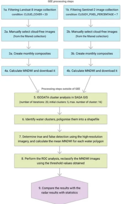
The processing steps were as follows (Figure4):
1. Cloud-free Landsat 8 and Sentinel-2 data were selected and MNDWI images were calculated and downloaded with GEE.
2. Performed cluster analysis on the MNDWI data with an optimized ISODATA algorithm [57]
in SAGA GIS 5.0 open-source software (Departments for Physical Geography, Hamburg and Göttingen, Germany) with default settings (number of iterations: 20, initial clusters: 5, maximum number of clusters: 16). Identified the cluster that represented surface water cover. Polygonised the resulting thematic raster layer.
3. Determined the true and false detection for each water polygon using the high-resolution imagery.
Calculated the mean MNDWI for each water polygon. As a result, we had a data table with one column of Boolean values and the MNDWI mean value for each water polygon. In other words, we obtained a Boolean value and an MNDWI mean value pair as the input for the ROC curve calculation.
4. Performed the ROC analysis. Reclassified the MNDWI images using the threshold values obtained via ROC.
5. Compared the results with the radar results with statistics.
Figure 4.Flowchart of the data processing steps applied to the Landsat 8 OLI and Sentinel-2 MSI data.
The processing steps (1–4) were done in the GEE application. Steps 5–9 were done outside of GEE.
3. Results
3.1. Monthly Surface Water Cover
It is challenging to detect changes in the frequency and permanency of surface water cover due to the high natural variability of wetland ecosystems. In Figure5, we plotted monthly surface water cover in terms of the ascending and descending paths. Half of the monthly surface water cover values were in the range of 400–900 ha. If we consider only the values below 1000 ha, and thus exclude any extreme values, the frequency distribution appears to be relatively normal, i.e., it more or less forms a bell curve. Owing to the outlying end-of-winter or springtime water cover peaks, there was a large difference between the average and median values. The minimum monthly water coverage occurs in the August–October period of each year. There were multiple differences between the spring peaks and the end-of-summer/autumn minimums.
Figure 5. Density function (top) and box plot (bottom) of monthly water coverage—(WEKA K-Means_DESC-water coverage obtained from the classification of images captured on the descending path; WEKA K-Means_ASC—the same procedure for the ascending path. The blue represents arithmetic averages.
The spring peaks in 2016 and 2017 were less prominent compared with those of the other years.
Interestingly, even in wetter years, the summer-autumn water coverage fell back into the mostly 400–900 ha range despite the higher springtime peak. The effect of the lack of refilling is clearly represented by the summer values recorded for 2017, the lowest in the dataset, because the low 2016 springtime peak was followed by a subsequent low peak in 2017 (Figure6). This can be supported by the low rainfall levels recorded for the period from August 2016 to May 2017, which were generally typically below average. The average surface water cover was 529 ha for the descending path (based on 253 Sentinel-1 images) and 633 ha for the ascending path (based on 300 images) in our study period.
Figure 6.Monthly Sentinel-1 (both ascending and descending paths), Sentinel-2, and Landsat 8 water cover time-series between October 2014 and November 2018.
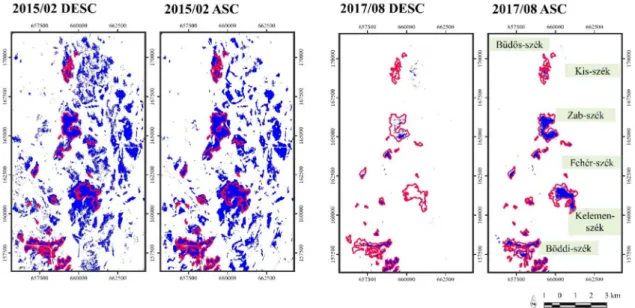
The largest surface water cover was in February 2015, with a coverage of 2628 ha (descending path;
all the following figures are for the descending path) (Figure7), largely due to the good precipitation amount and three-month ratio value for July 2014 (see Figure2). This had shrunk to 1/6 of the initial coverage (415 ha) by August. The 2016 peak was 1579 ha, the 2017 peak 800 ha, and the 2018 peak 1938 ha, all of which occurred in March. The very low ha value for the spring of 2017 was due to the low precipitation amount during the period from August 2016 to March 2017, whereas, due to the favorable circumstances experienced from May 2017, the peak value for 2018 was the second highest for the entire study period. The minimum coverages were in September 2016 (575 ha), August 2017 (141 ha), and November 2018 (283 ha) (Figure6), which are in line with the precipitation values shown in Figure2. In partial sum, taking the period between 2015 and 2017, there was a 6.3-, 2.7-, and 5.7-fold difference between the minimum and maximum water coverage, respectively. The extreme natural variability that we measured corresponds well with previous Landsat-based research in our study area [6,16]. Without the knowledge of this variability, we cannot analyze the real changes that occur in the sensitive wetland areas.
Figure 7. Water cover maps: the peak coverage as of February 2015 and the minimum coverage as of August 2017. DESC: descending path; ASC: ascending path; the average boundaries of the largest water patches/lakes for the examined period are depicted using red lines.
There was no significant difference between the surface water cover calculated from the descending and ascending paths separately (Pearson’sr=0.96). However, there were some larger discrepancies between the two, with a difference of fewer than 15 ha in 24% (8) of the cases and under 50 ha in 56%
(19) of the cases, and a difference of over 100 ha in 44% (15) of the cases. In four monthly periods, there was a difference of over 300 ha. For example, in February and March of 2015, there were differences in surface water coverage of 257 and 312 ha, respectively, and the average difference between the ascending and descending paths was 110 ha. As we used monthly averages, it was important to know which days of the months we had acquisitions for and how many images were available for months when there were high wind speeds. Moreover, because the surface water coverage in the study area can change substantially even in a single month, the different times of the acquisitions for the descending and ascending paths could also have resulted in some discrepancies. Owing to the windy weather, there were no good data for certain months, meaning we had data gaps for November and December of 2014; January, April, and September of 2015; August of 2016; and December of 2017 for the descending path, and gaps for April and July of 2015 and January, February, and October of 2016 for the ascending path.
3.2. Validation Using MNDWI
We used all the available cloud-free Landsat 8 (N = 21) and Sentinel-2 (N = 23) images for validation of the radar results (Figure4). We calculated the linear regressions and correlations and performed a significance test (Figure 8). The analysis yielded significant connections (p < 0.001 andp<0.01) with good correlations. The connection with the Sentinel-2 data was slightly lower than that with the Landsat 8 data. Pearson’s correlations were between 0.79 and 0.96, whereas the rank-based Spearman’s correlations were lower (0.54–0.80) (Table2). Owing to the highly influential peak data points (maximum water coverage), the sample distribution is non-Gaussian, meaning the nonparametric Spearman’s correlation is the standard because it does not require the distribution to be normal.
Figure 8.Linear regression lines (blue lines) between monthly water coverage (in ha) calculated from the radar and the water index (reference) data—the red line is an exponential fit, but for informative purposes only; L8_MNDWI and S2_MNDWI are for the water cover data derived from Landsat 8 and Sentinel-2 images, respectively.
Table 2.Pearson’s and Spearman’s correlation coefficients for the linear regressions.
Statistical Connections Linear Regressions
Pearson’s r-value Spearman’sρ-value
wekaKMeans_DESC ~ L8_MNDWI 0.95 *** 0.73 ***
wekaKMeans_ASC ~ L8_MNDWI 0.96 *** 0.80 ***
wekaKMeans_DESC ~ S2_MNDWI 0.80 *** 0.69 ***
wekaKMeans_ASC ~ S2_MNDWI 0.79 *** 0.54 **
** Significant at the 1% level,p<0.01. *** Significant at the 0.1% level,p<0.001.
It is clear from the results that there was a connection between the radar results and the MNDWI results, which validates our Sentinel-1 C-SAR-based method as an appropriate tool for surface water detection in wetlands. However, there is substantial uncertainty with our results due to the larger differences in the calculated monthly surface water coverage (in some cases), which was expected given the different types of data operating in completely different sections of the electromagnetic spectrum.
In the next phase of the investigation, we attempted to use the ROC method for the Sentinel-1 data, but the results were negative (area under the curve (AUC)=0.135 for both dates). AUC represents the
degree or measure of separability and informs us about the extent to which the model is capable of distinguishing between classes. The higher the AUC, the better the model. Herein, the AUC value was 0.5 for a random predictor (diagonal line on the plot), which means true and false detection cannot be differentiated. The AUC should thus be well above 0.5. For the MNDWI data, the AUC value was above 0.7, which indicates a good measure of separability (Table3, Figure9). The wetland water coverage threshold obtained from the ROC analysis was MNDWI≥0.625 for the Landsat 8 OLI and MNDWI≥0.570 for the Sentinel-2 MSI. According to Du et al. [55], the ideal MNDWI threshold value for Sentinel-2 is much lower, at between 0.2 and 0.35. The difference here was that we could only sense shallow waters, meaning this was a unique natural environment that meant the results were also unique.
Table 3.Threshold limits obtained from the ROC curve analysis.
Data Threshold Limit AUC
Landsat 8 (15 August 2016) MNDWI=0.593 0.73
Landsat 8 (27 March 2017) MNDWI=0.656 0.76
Sentinel-2 (8 August 2016) MNDWI=0.553 0.78
Sentinel-2 (29 March 2017) MNDWI=0.586 0.74
Sentinel-1 (August 2016) σ0=−15.53 dB 0.135 Sentinel-1 (March 2017) σ0=−17.87 dB 0.135
Figure 9.ROC curves calculated for the Sentinel-1 C-VV, Sentinel-2 Modified Normalized Difference Water Index (MNDWI), and Landsat 8 MNDWI data using a Pléiades image (08/09/2016) and WorldView-3 (03/17/2017) high-resolution image obtained via Google Earth Pro; unlike the MNDWI data, no appropriate threshold limit was found for the radar data. TPR denotes true positive rate, and FPR denotes false positive rate.
For most cases, there was no significant difference between descending path and ascending path data, as noted above. The water coverage curves clearly move in line, merging most of the time, with some exceptions (Figure6). There was some discrepancy for the descending path in February, April, and August of 2017, when the water coverage sharply dropped, before it returned to the level of the ascending path the following month. The main factors here were bad image quality, low contrast because of wind shear, and high speckle noise.
In February 2017, five images were available for the descending path and 10 for the ascending path, with wind speeds of 5.97 and 9.09 km/h, respectively. In April 2017, four images were available for the descending path and 10 for the ascending path, with wind speeds of 10.49 and 7.07 km/h, respectively.
In August 2017, six images were available for the descending path and 10 for the ascending path, with wind speeds of 5.18 and 9.58 km/h, respectively. It was concluded that it was likely that the lower number of images for the descending path played a role in the bad image quality. There was a significant difference in water coverage between January and February of 2016, with only two images available for January and three for February for the descending path, meaning these data are less trustworthy. Here, the wind speeds were 8.44 and 11.31 km/h, respectively. There were higher wind speeds (18.19 km/h in January and 19.24 km/h in February) for the ascending path for this period.
To summarize, it can be stated that the image quality was slightly better for the ascending path in the study area, mainly because more images were available for each month compared with the descending path. The minimum and maximum coverage fell in the same month for both satellite paths, but they differed in terms of the extent of the coverage. The main factors here were wind-induced waves, bad image quality, and the different number of images for the two satellite paths.
We also checked how much the winter snow and ice coverage affected the detection of the surface water coverage for months such as January 2017, when there was significant ice coverage. Here, there was no difference in the surface water coverage results between the Sentinel-1 radar and Sentinel-2 and Landsat 8 optical images, which is also visually evident (Figure10).
Figure 10.Comparison of Sentinel-1 radar, Sentinel-2, and Landsat 8 surface reflectance composites for January 2017—RGB: 7/4/3 and RGB: 12/8/4 both denote the combination of SWIR/NIR/visible red satellite image bands; SWIR: short-wave infrared band atλ=2.1µm; NIR: near-infrared band atλ=0.8–0.9µm.
The explanation here is that ice forms with a more or less smooth surface similar to calm water surfaces, meaning it does not affect our ability to delineate any water coverage that is under the ice. In contrast, MNDWI was sensitive to snow coverage, with high index values as with the water coverage, meaning the snow was misclassified as water. Therefore, it is better not to use snowy images for optical data. The optical false-color composites are more interesting here (the snow cover is cyan colored, and the ice cover on the saline lakes is highlighted using dark-blue shading). The Sentinel-2 image is from 8 January; the Landsat 8 median image consists of three images (6, 15, and 22 January), and the snow coverage differs from that of the Sentinel-2 image.
4. Discussion
Our conclusions are backed by the results of domestic research groups that examined the integration potential of Sentinel-1 C-SAR and Sentinel-2 MSI optical data for mapping inland excess water [54,58,59]. This is a local phenomenon that represents unwanted surface water patches on agricultural land, especially in the melting period at the end of winter and during spring, which has multiple causes [54]. It was also concluded that radar and optical data can supplement each other effectively, because the water coverages calculated from radar and optical data were a good match.
To illustrate this, we created a map that compares two Sentinel-1 radar composites (ascending and descending paths) from February 2015 with a Landsat 8 false-color composite from 18 February 2015 (Figure11). The relationship between the ascending path data and the multispectral image is stronger.
A mixed classification approach that uses radar and optical data as inputs may be a promising idea, although there are far less cloud-free optical data available. However, the goal of the study was only to have operational monitoring preferably without any data gaps.
Figure 11.Comparison of Sentinel-1 radar and Landsat 8 surface reflectance composites for February 2015—RGB: 7/4/3 denotes the combination of SWIR/NIR/visible red satellite image bands; SWIR:
short-wave infrared band atλ=2.1µm; NIR: near-infrared band atλ=0.8–0.9µm.
The biggest issue is the roughening effect of wind on water features when delineating water using SAR imagery. Alsdorf et al. [19] have provided a possible solution by using multi-temporal
interferometric SAR phase-coherence, which is based on lower coherence over water (e.g., the scattering characteristics of water surfaces continually change with waves resulting in poor repeat-pass coherence) relative to the surrounding land surface. This approach requires the coherence of surrounding surfaces to remain greater, but this condition is not typically met for orbital repeat cycles greater than a few days [60]. It is six days for Sentinel-1 [8]. Unfortunately, Sentinel-1 SLC data cannot currently be ingested, as Earth Engine does not support images with complex values due to the inability to average them during pyramiding without losing phase information [61]. However, wind roughening effects likely had negligible effects on our ability to delineate water because of below-the-threshold wind speeds experienced in our study area most of the time: 8.4 km/h on average for both ascending and descending paths. There were relatively above-average wind speeds in April 2015 (18.1 km/h), in July 2015 (20.4 km/h), and in January and February 2016 (18.2 and 19.2 km/h, respectively) for the ascending path, and in April 2015 (27.3 km/h) and in December 2017 (19.5 km/h) for the descending path (Figure12).
Figure 12.Average wind speed time-series between October 2014 and November 2018. The average wind speed was calculated for the days of Sentinel-1 image acquisitions (ascending and descending paths separately). In months where the wind threshold was exceeded for all pixels at all acquisitions, wind speed was calculated without applying the wind filtering. For the rest, wind speed was calculated by applying the wind filtering because we wanted the average wind speed only for the unmasked pixels. The black line shows the average wind speed of 8.39 km/h.
The water cluster centers for VV values were in the range between−15 and−25 decibels even for the small subset of anomalously-high-wind-speed months, which is much higher than the−6 to
−15 dB range recommended by Manjusree el al. [21] as an optimum range for the classification of water in VV polarizations. The variable cluster centers for water cover confirm that using a single σ0threshold value is not adequate for accurate water cover delineation because there are numerous differences between acquisitions (like incidence angle, wind speed, and the wetland ecosystem also dynamically changing) that are unique to that particular scene [26,27]. However, we found that the variation in incidence angle was less than 1◦over the entire study area: the average incidence angle was 37◦. The fluctuations in water cluster centers were stable with an average of−20 decibels for both ascending and descending paths. The higher the VV cluster center values for water cover, the higher is the chance of misclassification because of the lower contrast of water features with their surroundings.
There is an additional factor to consider.
Bolanos et al. [26] found in their study that some water features delineated with SAR did not appear on the optical imagery (especially, when its resolution was 5 meters or more). They argued that these could be considered false positives, but since SAR is more sensitive to water content, these areas could also be areas of low vegetation (where the vegetation cover is not high enough to influence backscatter, but its chlorophyll content does influence reflectance) with particularly high water content.
In contradiction, Slagter et al. [62] found that water cover under a vegetation canopy cannot be detected for herbaceous wetlands with higher vegetation coverage using Sentinel-1 SAR data. This was the case in our study. This was especially true for the so-called “black saline lakes,” which were also present in our study area, that have high biological production and high suspended organic matter content that colors their water to yellow-brownish. They are in a transitioning state to become freshwater marshes with rich marsh vegetation (reeds and grasses) and less open water [20]. Therefore, the water cover under the vegetation canopy was not detected with SAR because of the higher backscatter in these areas. Thus, the MNDWI-based water area extent was generally higher than the calculated water extent from SAR data.
5. Conclusions
We developed a Sentinel-1 C-SAR-based surface water cover detection method that is mainly independent of weather conditions, with the exception of the wind shear that induces waves on the otherwise smooth water surfaces and leads to increased backscatter due to the roughening effects.
There was a good connection between the Sentinel-1 C-SAR, Landsat 8, and Sentinel-2 MNDWI results, which validated our method as an appropriate tool for surface water detection in wetlands.
Surface water coverage detection was based on the WEKA K-Means clustering algorithm. ROC analysis proved to be useless for radar data because no threshold limit was found. In contrast, ROC analysis was found to be excellent for detecting water coverage using MNDWI threshold limits.
The radar results were not affected by snow and ice coverage in the winter months of certain years (e.g., January 2017). In contrast, the MNDWI results of the optical images were highly sensitive to snow coverage.
There were no significant differences between the images from the ascending and descending satellite paths. In some cases, the image quality was bad due to wind-induced waves and possible speckle artefacts, which are often falsely classified as water cover.
Wind roughening effects and incidence angle variations likely had negligible effects on our ability to delineate water in the study area.
The water cluster centers for VV values were in the range between−15 and−25 decibels with an average of−20 decibels for both ascending and descending paths.
Water cover area was higher for MNDWI than radar data: likely because of the inability to detect water cover under the vegetation canopy because of the higher radar backscatter in these areas.
Unfortunately, radar-based water detection methods also have their limitations, but we can obtain more detailed insight into changes in the surface water coverage of wetlands using them.
Utilizing cloud processing platforms such as GEE, we can speed up the geoprocessing and analysis of Sentinel-1 C-SAR data on a mass scale. This makes continuous automatic wetland monitoring possible, which, in turn, could help with managing and protecting wetlands more effectively for national and international nature conservation.
Future work should involve extending the validation process to include field surveys and aerial surveys using unmanned aerial vehicles because this initial study was not comprehensive enough to fully explain the discrepancies.
Author Contributions: Conceptualization: A.G.; data management and data processing: A.G.; methodology:
A.G. and F.K.; investigation: A.G. and F.K.; validation: A.G.; visualization: A.G.; writing—original draft: A.G.
and F.K.; writing—editing: A.G. and F.K.; funding acquisition: F.K. Both authors have read and agreed to the published version of the manuscript. All authors have read and agreed to the published version of the manuscript.
Funding:The research has been supported by the University of Szeged. The research has been supported by the Hungarian National Research Fund (OTKA K 124648).
Acknowledgments: This research was supported by the Interreg-IPA Cross-border Cooperation Program Hungary–Serbia and co-financed by the European Union (IPA) under the project HUSRB/1602/11/0057 entitled WATERatRISK (Improvement of drought and excess water monitoring for supporting water management and mitigation of risks related to extreme weather conditions).
Conflicts of Interest:The authors declare no conflicts of interest.
Appendix A
Link to the GEE scripts we used for processing and downloading Sentinel-1 C-SAR data. You need to sign up for GEE to use them if you have not done so already. Check the README first. You have only reading rights to the scripts. https://code.earthengine.google.com/?accept_
repo=users/gulandras90/inlandExcessWater. The code also available in this repository: https:
//github.com/SalsaBoy990/gee_s1_sar_wetlands. The ROC curve calculating R code with the input data supplied (in a zip file).https://drive.google.com/open?id=1ePLf99Hwp9BU8s7qP_3xxPGf85Z6FpAO.
R code used for calculating statistics with the input data tables supplied (in a zip file). https:
//drive.google.com/open?id=1uND3HtyIb36x7JTANHWrdLpT2NW2_UJx. Radar data used in the study (in a zip file).https://drive.google.com/open?id=1FJJMXVaqwF9uc8DBgBsUJOw1KiJrVVKX.
References
1. Ramsar Sites of Hungary. Available online:https://www.ramsar.org/wetland/hungary(accessed on 27 March 2020).
2. IPCC. Climate change 2013. The Physical Science Basis; Stocker, T.F., Qin, D., Plattner, G.-K., Tignor, M.M.B., Allen, S.K., Boschung, J., Nauels, A., Xia, Y., Bex, V., Midgley, P.M., Eds.; Part of the working group I contribution to the fifth assessment report of the Intergovernmental Panel on Climate Change.
Intergovernmental Panel on Climate Change. 2013. Available online: https://www.ipcc.ch/site/assets/
uploads/2018/03/WG1AR5_SummaryVolume_FINAL.pdf(accessed on 27 March 2020).
3. Mez˝osi, G.; Blanka, V.; Ladányi, Z.S.; Bata, T.; Urdea, P.; Frank, A.; Meyer, B. Expected mid- and long-term changes in drought hazard for the South-Eastern Carpathian Basin.Carpathian J. Earth Environ. Sci.2016,11, 355–366.
4. Dawson, T.P.; Berry, P.M.; Kampa, E. Climate change impacts on freshwater wetland habitats.J. Nat. Conserv.
2003,11, 25–30. [CrossRef]
5. Erwin, K.L. Wetlands and global climate change: The role of wetland restoration in a changing world.Wetl.
Ecol. Manag.2009,17, 71–84. [CrossRef]
6. Kovács, F. Változékonyságértékelése vizesél˝ohelyeken–M ˝uholdképek alapján (Assessment of instability in a wetland area with remote sensing methods).Hidrol. Közlöny2009,89, 57–61. (in Hungarian).
7. Rosenqvist, A.; Finlayson, C.M.; Lowry, J.; Taylor, D. The potential of long-wavelength satellite-borne radar to support implementation of the Ramsar Wetlands Convention.Aquat. Conserv. Mar. Freshw. Ecosyst.2007, 17, 229–244. [CrossRef]
8. Torres, R.; Snoeij, P.; Geudtner, D.; Bibby, D.; Davidson, M.; Attema, E.; Potin, P.; Rommen, B.; Floury, N.;
Brown, M.; et al. GMES Sentinel-1 mission.Remote Sens. Environ.2012,120, 9–24. [CrossRef]
9. Szczepankiewicz, K.; Malanowski, M.; Szczepankiewicz, M. Passive radar parallel processing using general-purpose computing on graphics processing units. Int. J. Electron. Telecommun.2015,61, 357–363.
[CrossRef]
10. Yin, Q.; Wu, Y.; Zhang, F.; Zhou, Y. GPU-based soil parameter parallel inversion for PolSAR data.Remote Sens.
2020,12, 415. [CrossRef]
11. Chi, M.; Plaza, A.; Benediktsson, J.A.; Sun, Z.; Shen, J.; Zhu, Y. Big data for remote sensing: Challenges and opportunities.Proc. IEEE2016,104, 2207–2219. [CrossRef]
12. Liu, P.; Di, L.; Du, Q.; Wang, L. Remote sensing big data: Theory, methods and applications.Remote Sens.
2018,10, 711. [CrossRef]
13. Gorelick, N.; Hancher, M.; Dixon, M.; Ilyushchenko, S.; Thau, D.; Moore, R. Google Earth Engine:
Planetary-scale geospatial analysis for everyone.Remote Sens. Environ.2017,202, 18–27. [CrossRef]
14. Kumar, L.; Mutanga, O. Google Earth Engine applications since inception: Usage, trends, and potential.
Remote Sens.2018,10, 1509. [CrossRef]
15. Beck, H.E.; Zimmermann, N.E.; McVicar, T.R.; Vergopolan, N.; Berg, A.; Wood, E.F. Present and future Köppen-Geiger climate classification maps at 1-km resolution.Sci. Data2018,5, 180214. [CrossRef] [PubMed]
16. Kovács, F. GIS analysis of short and long term hydrogeographical changes on a nature conservation area affected by aridification.Carpathian J. Earth Environ. Sci.2013,8, 97–108.
17. Bihari, Z.; Babolcsay, G.; Bartholy, J.; Ferenczi, Z.; Kerényi, J.; Haszpra, L.;Újváry, K.; Kovács, T.; Lakatos, M.;
Németh,Á.; et al. Éghajlat (Climate). In Magyarország Nemzeti Atlasza 2. Kötet: Természeti Környezet (Hungarian National Atlas, Nature Environment); Kocsis, K., Horváth, G., Keresztesi, Z., Nemerkényi, Z., Eds.; MTA CSFK Földrajztudományi Intézet: Budapest, Hungary, 2018; pp. 58–69. Available online:
http://www.nemzetiatlasz.hu/MNA/MNA_2_5.pdf(accessed on 27 March 2020). (In Hungarian)
18. Kovács, F.; Gulácsi, A. Spectral index-based monitoring (2000–2017) in lowland forests to evaluate the effects of climate change.Geosciences2019,9, 411. [CrossRef]
19. Alsdorf, D.E.; Rodríguez, E.; Lettenmaier, D.P. Measuring surface water from space. Rev. Geophys.2007, 45, 478. [CrossRef]
20. ÉrdinéSzekeres, R.Szikes tavak (Saline Lakes); Környezetvédelmi Minisztérium Természetvédelmi Hivatala:
Budapest, Hungary, 2002; pp. 10–11. (in Hungarian)
21. Manjusree, P.; Prasanna Kumar, L.; Bhatt, C.M.; Rao, G.S.; Bhanumurthy, V. Optimization of threshold ranges for rapid flood inundation mapping by evaluating backscatter profiles of high incidence angle SAR images.
Int. J. Disaster Risk Sci.2012,3, 113–122. [CrossRef]
22. Westerhoff, R.S.; Kleuskens, M.P.H.; Winsemius, H.C.; Huizinga, H.J.; Brakenridge, G.R.; Bishop, C.
Automated global water mapping based on wide-swath orbital synthetic-aperture radar. Hydrol. Earth Syst. Sci.2013,17, 651–663. [CrossRef]
23. White, L.; Brisco, B.; Pregitzer, M.; Tedford, B.; Boychuk, L. RADARSAT-2 Beam Mode Selection for Surface Water and Flooded Vegetation Mapping.Can. J. Remote Sens.2014,40, 135–151. [CrossRef]
24. Hong, S.; Jang, H.; Kim, N.; Sohn, H.-G. Water area extraction using RADARSAT SAR imagery combined with landsat imagery and terrain information.Sensors2015,15, 6652–6667. [CrossRef]
25. Li, J.; Wang, S. An automated method for mapping inland surface waterbodies with Radarsat-2 imagery.
Int. J. Remote Sens.2015,36, 1367–1384. [CrossRef]
26. Bolanos, S.; Stiff, D.; Brisco, B.; Pietroniro, A. Operational surface water detection and monitoring using Radarsat-2.Remote Sens.2016,8, 285. [CrossRef]
27. Liang, J.; Liu, D. A local thresholding approach to flood water delineation using Sentinel-1SAR imagery.
ISPRS J. Photogramm. Remote Sens.2020,159, 53–62. [CrossRef]
28. Sokol, J.; Ncnairn, H.; Pultz, T.J. Case studies demonstrating the hydrological applications of C-band multipolarized and polarimetric SAR.Can. J. Remote Sens.2004,30, 470–483. [CrossRef]
29. De Zan, F.; Guarnieri, A.M. TOPSAR: Terrain Observation by Progressive Scans. IEEE Trans. Geosci.
Remote Sens.2006,44, 2352–2360. [CrossRef]
30. Brisco, B. Mapping and monitoring surface water and wetlands with synthetic aperture radar. InRemote Sensing of Wetlands: Applications and Advances; Tiner, R., Lang, M., Klemas, V., Eds.; CRC Press: Boca Raton, FL, USA, 2015;
pp. 119–136.
31. Hess, L.L.; Melack, J.M.; Simonett, D.S. Radar detection of flooding beneath the forest canopy: A review.Int.
J. Remote Sens.1990,11, 1313–1325. [CrossRef]
32. Engman, E.T. Remote sensing applications to hydrology: Future impact.Hydrol. Sci. J.1996,41, 637–647.
[CrossRef]
33. Lang, M.W.; Kasischke, E.S. Using C-band synthetic aperture radar data to monitor forested wetland hydrology in Maryland’s coastal plain, USA.IEEE Trans. Geosci. Remote Sens.2008,46, 535–546. [CrossRef]
34. Kasischke, E.S.; Melack, J.M.; Dobson, M.C. The use of imaging radars for ecological applications – A review.
Remote Sens. Environ.1997,59, 141–156. [CrossRef]
35. Bourgeau-Chavez, L.L.; Kasischke, E.S.; Brunzell, S.M.; Mudd, J.P.; Smith, K.B.; Frick, A.L. Analysis of space-borne SAR data for wetland mapping in Virginia riparian ecosystems.Int. J. Remote Sens.2001,22, 3665–3687. [CrossRef]
36. Baghdadi, N.; Bernier, M.; Gauthier, R.; Neeson, I. Evaluation of C-band SAR data for wetlands mapping.
Int. J. Remote Sens.2001,22, 71–88. [CrossRef]
37. Google Earth Engine: A planetary-scale platform for Earth science data & analysis. Available online:
https://earthengine.google.com/(accessed on 27 March 2020).
38. ESA step – science toolbox exploitation platform. Available online:http://step.esa.int/main/doc/tutorials/
(accessed on 27 March 2020).
39. Small, D. Flattening Gamma: Radiometric terrain correction for SAR imagery.IEEE Trans. Geosci. Remote Sens.
2011,49, 3081–3093. [CrossRef]
40. Weiß, T. SAR-pre-processing documentation. 2018. Personal communication. Available online:
https://buildmedia.readthedocs.org/media/pdf/multiply-sar-pre-processing/get_to_version_0.4/multiply- sar-pre-processing.pdf(accessed on 27 March 2020).
41. Ulaby, F.T.; Moore, R.K.; Fung, A.K.Microwave Remote Sensing: Active and Passive. Volume 2, Radar Remote Sensing and Surface Scattering and Emission Theory; Addison-Wesley: Reading, MA, USA, 1982; p. 608.
42. Hird, J.N.; DeLancey, E.R.; McDermid, G.J.; Kariyeva, J. Google Earth Engine, Open-Access satellite data, and machine learning in support of large-area probabilistic wetland mapping.Remote Sens.2017,9, 1315.
[CrossRef]
43. Elyouncha, A.; Neyt, X.; Stoffelen, A.; Verspeek, J. Assessment of the corrected CMOD6 GMF using scatterometer data. InRemote Sensing of the Ocean, Sea Ice, Coastal Waters, and Large Water Regions; Browse Proceedings: Toulouse, France, 2015; p. 11.
44. Onstott, R.; Shuchman, R. Sar measurements of sea ice. InSynthetic Aperture Radar Marine User’s Manual;
Jackson, C.R., Apfel, J.R., Eds.; NOAA, U.S. Department of Commerce: Washington, DC, USA, 2004;
pp. 81–115.
45. Shokr, M.; Sinha, N.Sea Ice: Physics and Remote Sensing; American Geophysical Union, John Wiley & Sons, Inc.: Hoboken, NJ, USA, 2015; pp. 325–326.
46. Saha, S.; Moorthi, S.; Pan, H.-L.; Wu, X.; Wang, J.; Nadiga, S.; Tripp, P.; Kistler, R.; Woollen, J.; Behringer, D.;
et al. The NCEP climate forecast system reanalysis.Bull. Am. Meteorol. Soc.2010,91, 1015–1057. [CrossRef]
47. Lee, J.S. Digital image enhancement and noise filtering by use of local statistics.IEEE Trans. Pattern Anal.
Mach. Intell.1980,PAMI-2, 165–168. [CrossRef]
48. Lee, J.S. Refined filtering of image noise using local statistics.Comput. Vis. Graph. Image Process.1981,15, 380–389. [CrossRef]
49. Yommy, A.S.; Liu, R.; Wu, S. SAR image despeckling using refined Lee filter. In7th International Conference on Intelligent Human-Machine Systems and Cybernetics (IHMSC); IEEE: Hangzhou, China, 2015; pp. 260–265.
[CrossRef]
50. Arthur, D.; Vassilvitskii, S. k-means++: The advantages of carefull seeding. In Proceedings of the Eighteenth Annual ACM-SIAM Symposium on Discrete Algorithms: Society for Industrial and Applied Mathematics, Philadelphia, PA, USA, January 2007; pp. 1027–1035. Available online:https://theory.stanford.edu/~{}sergei/
papers/kMeansPP-soda.pdf(accessed on 27 March 2020).
51. McFeeters, S.K. The use of the Normalized Difference Water Index (NDWI) in the delineation of open water features.Int. J. Remote Sens.1996,17, 1425–1432. [CrossRef]
52. Xu, H. Modification of normalised difference water index (NDWI) to enhance open water features in remotely sensed imagery.Int. J. Remote Sens.2006,27, 3025–3033. [CrossRef]
53. Li, W.; Du, Z.; Ling, F.; Zhou, D.; Wang, H.; Gui, Y.; Sun, B.; Zhang, X. A Comparison of Land Surface Water Mapping Using the Normalized Difference Water Index from TM, ETM+and ALI.Remote Sens. 2013,5, 5530–5549. [CrossRef]
54. Van Leeuwen, B.; Tobak, Z.; Kovács, F.; Sipos, G. Towards a continuous inland excess water flood monitoring system based on remote sensing data.J. Environ. Geogr.2017,10, 9–15. [CrossRef]
55. Du, Y.; Zhang, Y.; Ling, F.; Wang, Q.; Li, W.; Li, X. Water bodies’ mapping from Sentinel-2 imagery with Modified Normalized Difference Water Index at 10-m spatial resolution produced by sharpening the SWIR band.Remote Sens. 2016,8, 354. [CrossRef]
56. ROC curve, R script. Available online:http://oku.edu.mie-u.ac.jp/~{}okumura/stat/ROC.html(accessed on 29 March 2020).
57. Memarsadeghi, N.; Mount, D.M.; Netanyahu, N.S.; Moigne, J.L. A fast implementation of the ISODATA clustering algorithm.Int. J. Comput. Geom. Appl.2007,17, 71–103. [CrossRef]
58. Vekerdy, Z.; Qiu, Y.; Csorba,Á.; Czakó-Gál, E.; van Leeuwen, B. Belvíztérképezés Sentinel-1és Sentinel-2 képek integrációjával (Inland excess water mapping with the integration of Sentinel-1 and Sentinel-2 imagery.). In Proceedings of the FÉNY-TÉR-KÉP Konferencia, Gárdony, Hungary, 15–16 November 2018;
Available online:https://geoiq.hu/download/1971/(accessed on 1 May 2020). (in Hungarian).
59. Van Leeuwen, B.; Tobak, Z.; Kovács, F. Sentinel-1 and -2 Based near Real Time Inland Excess Water Mapping for Optimized Water Management.Sustainability2020,12, 2854. [CrossRef]
60. Smith, L.C.; Alsdorf, D.E. Control on sediment and organic carbon delivery to the Arctic Ocean revealed with space-borne synthetic aperture radar: Ob’ River, Siberia.Geology1998,26, 395–398. [CrossRef]
61. Google Earth Engine Sentinel-1 Algorithms. Available online:https://developers.google.com/earth-engine/
sentinel1(accessed on 1 May 2020).
62. Slagter, B.; Nandin-Erdene, T.; Andreas, V.; Johannes, R. Mapping wetland characteristics using temporally dense Sentinel-1 and Sentinel-2 data: A case study in the St. Lucia wetlands, South Africa.Int. J. Appl. Earth Obs. Geoinf.2020,86, 102009. [CrossRef]
©2020 by the authors. Licensee MDPI, Basel, Switzerland. This article is an open access article distributed under the terms and conditions of the Creative Commons Attribution (CC BY) license (http://creativecommons.org/licenses/by/4.0/).