When rare species are not important: linking plot-based vegetation classifications and landscape-scale mapping in Australian savanna vegetation

(1)

This article is published with Open Access at www.akademiai.com DOI: 10.1556/168.2018.19.1.7

Introduction

Plant communities underpin many land management and policy decisions (Margules and Pressey 2000) and much sci- entific research (De Cáceres et al. 2015). Maps showing the

ping extensive landscapes, differences are distinguished by changes in the dominant species canopy cover, by vegetation structure and by geomorphological differences in the landscape (Küchler and Zonneveld 1988, Franklin 2013, Pedrotti 2013).

When rare species are not important: linking plot-based vegetation classifications and landscape-scale mapping in Australian savanna vegetation

E. Addicott

^1,2,3,6

, S. Laurance

³

, M. Lyons

^4,5

, D. Butler

¹

and J. Neldner

¹

1Queensland Herbarium, Mt. Coot-tha Road, Toowong, Department of Environment and Science, Queensland Government, QLD 4066, Australia

2Australian Tropical Herbarium, James Cook University, Cairns, QLD 4870, Australia

3Centre for Tropical Environmental & Sustainability Science (TESS) and College of Science and Engineering, James Cook University, P.O. Box 6811, Cairns, QLD 4870, Australia

4Centre for Ecosystem Science, School of Biological, Earth and Environmental Sciences, UNSW Australia, NSW 2052, Australia

5New South Wales Office of Environment and Heritage, NSW 1232, Australia

6Corresponding author. E-mail: eda.addicott@des.qld.gov.au

Keywords: Characteristic species; Landscape classification; Plant communities; Subsets; Vegetation structure.

Abstract: Plant communities in extensive landscapes are often mapped remotely using detectable patterns based on vegetation structure and canopy species with a high relative cover. A plot-based classification which includes species with low relative canopy cover and ignores vegetation structure, may result in plant communities not easily reconcilable with the landscape patterns represented in mapping. In our study, we investigate the effects on classification outcomes if we (1) remove rare species based on canopy cover, and (2) incorporate vegetation structure by weighting species’ cover by different measures of vegetation height. Using a dataset of 101 plots of savanna vegetation in north-eastern Australia we investigated first, the effect of removing rare species using four cover thresholds (1, 5, 8 and 10% contribution to total cover) and second, weighting species by four height measures including actual height as well as continuous and categorical transformations. Using agglomerative hierarchical clustering we produced a classification for each dataset and compared them for differences in: patterns of plot similarity, clustering, species richness and evenness, and characteristic species. We estimated the ability of each classification to predict species cover using generalised linear models. We found removing rare species at any cover threshold produced characteristic species appearing to correspond to landscape scale changes and better predicted species cover in grasslands and shrublands. However, in woodlands it made no difference. Using actual height of vegetation layer maintained vegetation structure, emphasised canopy and then sub-canopy species in clustering, and predicted species cover best of the height-measures tested. Thus, removing rare species and weighting species by height are useful techniques for identifying plant communities from plot-based classifications which are conceptually consistent with those in landscape scale mapping. This increases the confidence of end-users in both the classifications and the maps, thus enhancing their use in land management decisions.

Abbreviations: ALL–dataset consisting of the full species pool; C>1– dataset with species contributing >1% to TFC included;

C>5 – dataset with species contributing >5%; C>8 – dataset with species contributing >8%; C>10 – dataset with species contributing >10% to TFC included; IS – Indicator Species; ISA – Indicator Species Analysis; TFC – Total Foliage Cover.

(2)

ping process, it needs to incorporate the attributes used to differentiate mapped changes. Across extensive landscapes this means changes in species canopy cover and vegetation height.

These may be influenced by recurrent disturbance patterns, such as past land management practices. In savanna vegetation, fire history is particularly important as it can influence species assemblages and the structure of plant communities across the landscape (Miller and Murphy 2017). Therefore, communities need to be distinguished by species that respond to, and are indicative of, landscape scale changes rather than short-lived temporal dynamics or change driven by small scale phenomena such as micro-climatic differences.

Plot-based classifications using full species inventories will include non-dominant, occasional species in a dataset (here termed rare). However, the distribution of these rare species is difficult to predict for many possible reasons. For example, rarity may be because species are responding to localised variations in the environment below the scale of mapping (Kent 2012) or to past landscape disturbance history such as fire regimes. Species may also be rare in the dataset due to biases resulting from sampling designs (for example, seasonality). Thus, they contribute to ‘noise’ in the dataset from the view point of broad-scale vegetation classification, possibly masking the relationships of interest between vegetation samples at landscape levels (Kent 2012) and leading to plant communities defined at, and characterised by species responding to habitat changes at, scales below that of the mapping. This compromises the application of both the map and the quantitative classification as ecologists lose confidence in both if the plant communities do not relate to plausible ecological interpretation at the mapping scale.

Removing rare species that contribute to ‘noise’ in the dataset is often recommended and decisions on rarity are commonly based on frequency of occurrence (McCune and Grace 2002, Kent 2012). This, however, can be problematic in broad-scale mapping projects with vegetation plot locations chosen using a preferential sampling design. Such sampling designs are often used because plot locations may be constrained by factors such as accessibility and survey effort, resulting in map units, distinctive in terms of species and/or structure at the appro- priate scale, being represented by single plots. As a result, species dominating communities represented by single plots may occur once or twice in the dataset, and, if rare species are chosen based on low frequency, these dominant species are removed. The consequence is losing essential information about plant communities in the mapping and risking misclas- sification of their representative plots. An alternative is to remove species with rarity measured as consistently low contribution to cumulative abundance (Field et al. 1982, Grime 1998, Mariotte 2014).

Mapped plant communities classified using both floristic and structural components have the broadest application in both research and planning (Küchler and Zonneveld 1988).

Vegetation structure is a well-established feature for differentiating vegetation at landscape scales and is represented both vertically by vegetation layers within a community and horizontally by change in vegetation formations across the landscape (Küchler and Zonneveld 1988). Height of vegeta-

tion layers is commonly used in classification schemes to rep- resent this; for example, in Australia vegetation is classified using vegetation formations defined partly by layer height (ESCAVI 2003, Hnatiuk et al. 2009) whilst in other coun- tries authors may weight species by transformations of layer height (Leathwick et al. 1988, Hall 1992).

In this study, we specifically investigate two questions:

how does 1) removing rare species based on contribution to total foliage cover, and 2) weighting species cover by different measures of vegetation layer height, influence the classification outcomes of plant communities in tropical savanna vegetation on Cape York Peninsula, Australia. We discuss the relevance of these findings to classifications identifying landscape-scale plant communities.

Methods Study area

The Cape York Peninsula bioregion is a 120,000 km² area of the monsoon tropics of north-eastern Australia (Fig.

1). Our study encompasses the savanna vegetation occurring on the landscapes of ranges, hills and lowlands formed from Mesozoic to Proterozoic igneous rocks – a geomorphological category recognised in the state-wide landscape classifica-

Figure 1. Study area location. Area of the landscapes on igneous rocks in Cape York Peninsula bioregion, north eastern Australia, with main towns and study plot locations.

19 Appendix 2: Classification dendrograms as a result of removing species based on %

contribution to total foliage cover. Clusters labelled by species contributing >10% to the similarity of sites in a cluster.

Appendix 3: Dendrograms of each dataset classification after incorporating different height measures.

Tables

Figures

Figure 1. Study area location. Area of the landscapes on igneous rocks in Cape York

Peninsula bioregion, north eastern Australia, with main towns and study plot locations.

(3)

tion scheme used in Queensland (Sattler and Williams 1999).

These landscapes cover 5 500 km²on the Peninsula occurring from sea level to above 800 m with an annual average rainfall range of 1000 - 2000 mm. Eighty percent of rainfall occurs in the wet season between December and March (Horn 1995). Temperature ranges from an average monthly minimum of 14ºC in winter (July) to an average monthly maximum of 36ºC in summer (December) (http://www.bom.gov.au/climate/

averages/tables/ , accessed on 1st September 2016).

Data collation

We extracted vegetation plot data from the Queensland Government ‘CORVEG’ plot database. Data had been col- lected as part of a comprehensive vegetation survey and map-

which focused primarily on changes in vegetation structure and species changes in the canopy layer (Neldner and Howitt 1991, Bedward et al. 1992). In plots dominated by ground layer species, the average percent foliage cover for each species was calculated from 1 m² quadrats placed at 10 m in- tervals along the 50 m transect (five quadrats in total). Plots were deleted if they contained taxa identified only to family level which contributed >1% of TFC to a layer. This left a total of 101 plots comprising three main formations: grasslands (n = 14 plots), shrublands (n = 21 plots), and woodlands (n

= 66 plots). Grasslands refer to all ground layer communities and includes grasslands, sedgelands, and rock pavements with scattered herbs and forbs (Neldner et al. 2017). Taxa which were inconsistently identified were amalgamated to genus level and non-native species were excluded.

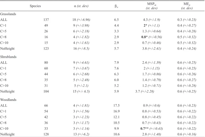
Table 1. Parameters and diversity of datasets. Subsets result from removing species based on % contribution to total foliage cover.

NoHeight = dataset used to weight species by height of vegetation layer. α = mean number of species per plot, βw = Whitaker’s beta diversity (Total number of species / α) – 1), MSPm = mean Margalef’s species richness index per plot; MEp = mean Pielou’s evenness index per plot. Species richness values significantly different to ALL are bolded, * p < 0.001, ** p < 0.01. ^ p=0.05.

Species α (st. dev) β_w MSP_m

(st. dev) ME_p

(st. dev) Grasslands

ALL 137 18 (+/-6.96) 6.5 4.3 (+/-1.9) 0.3 (+/-0.23)

C>1 49 9 (+/-3.98) 4.4 2* (+/-1.1) 0.4 (+/-0.27)

C>5 26 6 (+/-2.18) 3.3 1.3 (+/-0.64) 0.4 (+/-0.28)

C>8 16 4 (+/-1.82) 2.9 0.8* (+/-0.56) 0.5 (+/-0.32)

C>10 15 4 (+/-1.61) 2.9 0.7 (+/-0.46) 0.5 (+/-0.32)

NoHeight 123 16 (+/-8.5) 5.7 3.8 (+/-2.41) 0.4 (+/-0.24)

Shrublands

ALL 80 9 (+/-4.61) 7.9 2.4 (+/-1.39) 0.6 (+/-0.25)

C>1 60 7 (+/-3.67) 7.6 2 (+/-1.15) 0.6 (+/-0.25)

C>5 44 6 (+/-2.68) 6.3 1.7 (+/-0.86) 0.6 (+/-0.26)

C>8 35 5 (+/-2.48) 6.0 1.4 (+/-0.79) 0.6 (+/-0.27)

C>10 31 5 (+/-2.1) 5.2 1.2 (+/-0.71) 0.6 (+/-0.28)

NoHeight 104 15 (+/- 6.5) 5.9 3.7 (+/-2.28) 0.6 (+/-0.25)

Woodlands

ALL 66 4 (+/-1.81) 17.5 0.9 (+/-0.6) 0.6 (+/-0.23)

C>1 54 3 (+/-1.56) 16.9 0.8 (+/-0.53) 0.6 (+/-0.22)

C>5 42 3 (+/-1.23) 12.1 0.8 (+/-0.45) 0.6 (+/-0.22)

C>8 36 3 (+/-1.17) 10.5 0.7 (+/-0.43) 0.6 (+/-0.22)

C>10 33 3 (+/-1.14) 9.9 0.7** (+/-0.43) 0.6 (+/-0.22)

NoHeight 128 13 (+/-6.2) 10.6 2.8 (+/-1.48) 0.6 (+/-0.16)

(4)

to test for the effect of vegetation height. This dataset was 78 plots and 265 species (Table 1). We used the same 78 plots as a previous classification to allow comparisons with our final classification (work that was specific to another project and not included here). Fourteen plots were grassland, 16 were shrubland and 48 were woodland. This dataset included species in the canopy layer plus all other woody dominated layers with TFC of 10% or more (Neldner et al. 2017). Species in the ‘height’ dataset were excluded (from each layer) based on our analysis of rare species contribution to TFC (grasslands

<8% of TFC, shrublands <1%, woodlands <10% of TFC).

Using our ‘cover’ dataset we explored the effects on classification of removing rare species (defined here as their contribution to TFC) by defining four rarity thresholds; 1%, 5%, 8% and 10% contribution to TFC. These were determined a priori through an expert panel of regional mapping special- ists. We created four data subsets; C>1 = species contributing

>1% to TFC included, C>5 = species contributing >5%, C>8

= species contributing >8%, and C>10 = species contributing >10% to TFC included. The dataset consisting of the full species pool we termed ALL. Excluded species were below threshold levels for all plots and resulted in changes in community structure (Table 1). Following the advice of Anderson et al. (2011) we calculated beta diversity as variation in community structure amongst our samples using Whitaker’s beta- diversity calculation.

To explore the effects on classifications of weighting species by height of vegetation layer we used our ‘height’ dataset and four commonly used height-measures. These were;

height (Height) (Specht 1981, Hnatiuk et al. 2009); log10 (x + 1) of height (LogHeight) (Hall 1992, Wyse et al. 2014); an expert-based ranking of height given to each layer (RankHeight) (Leathwick et al. 1988); and foliage cover only with no height measure (NoHeight). Height was the average height in meters of each layer in the plot. For the RankHeights the expert panel provided the following ranks based on their perception of the ecological function of each layer in the formation: woodlands and shrublands - canopy layer = 3, emergent, sub-canopy, shrub and sub-shrub layers = 2; grasslands - ground layer = 3, emergent layer = 2. To weight species we multiplied the foliage cover of each species in a layer by the height-measure of the layer. Weighted species were summed across layers to give a total value per plot.

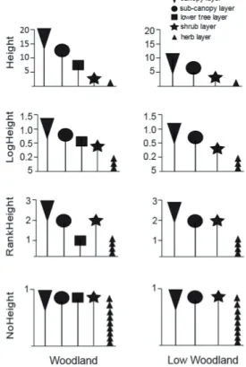
Weighting species by different height-measures changed the vegetation structure within and between plots (Fig. 2) and it is these effects on classifications that we test in this study.

NoHeight, LogHeight and RankHeight up-weighted the lower vegetation layers with respect to the canopy layer (Fig. 2). A NoHeight measure caused the most extreme change. Species in the lower layers of a plot had the same weighting as those in the canopy layer and structural differences between plots of different formations are eliminated (Fig. 2). LogHeight proportionally up-weighted the lower layers with respect to the canopy layer and reduces the structural differences between plots (Fig. 2). RankHeight weights species in different layers inconsistently and the outcomes are dependent on the value given by the expert panel. In addition, it eliminated all structural differences between formations (Fig. 2). Height

maintains vegetation structure both within a plot and between formations (Fig. 2).

Data analysis

We determined classifications for datasets using agglomerative hierarchical clustering, and internal evaluators to determine the level of cluster division (Aho et al. 2008). All analyses were undertaken in the software package PRIMER v6 (Clarke and Gorley 2006) or in the R environment (R Development Core Team 2014). To test the sensitivity of our results in removing rare species, we formed classifications for each dataset using two common combinations of similarity measure and clustering algorithms (Appendix 2). These were the Bray-Curtis similarity coefficient with Unweighted Pair Means Average linkage (UPGMA) (Kent 2012), and chord distance measure with flexible-β linkage (Knollova et al. 2005, Nezerkova-Hejcmanova et al. 2006, Roberts 2015).

In the latter, we used two levels of β. Beta = –0.25 has been used effectively in numerous classifications (Lotter et al.

2013, Mucina and Daniel 2013, Roberts 2015). Clarke et al.

(2014) recommend choosing a level of β that maximises the

20 Figure 2. Effects on species cover of weighting by vegetation height within and between plots. The height of the symbols represents the relative weighting of each layer compared with the canopy layer. Except for Height, the height-measures up-weighted the lower layers with respect to the canopy layer within a plot and reduced or eliminated height differences between vegetation formations. We used 2 plots from the study area as our examples. Height

= height in meters, LogHeight = log

10 ( x + 1)

of height, RankHeight = expert weightings for layers, NoHeight = no height included, foliage cover only. Vegetation layers labelled according to (Mucina et al. 2000).

Figure 2. Effects on species cover of weighting by vegetation height within and between plots. The height of the symbols represents the relative weighting of each layer compared with the canopy layer. Except for Height, the height-measures up- weighted the lower layers with respect to the canopy layer within a plot and reduced or eliminated height differences between vegetation formations. We used 2 plots from the study area as our examples. Height = height in meters, LogHeight = log10 ( x + 1) of height, RankHeight = expert weightings for layers, NoHeight = no height included, foliage cover only. Vegetation layers labelled according to Mucina et al. (2000).

(5)

cophenetic correlation between the distance matrix and the classification dendrogram, and in our datasets β was equal to 0.01. We therefore tested changes resulting from removing rare species with three different methods: 1) Bray-Curtis similarity with UPGMA, 2) chord distance with flexible-β at β = –0.25 and 3) chord distance with flexible-β at β = 0.01.

To determine cluster divisions, we used a combination of the SIMPROF routine (p<0.05) (Clarke et al. 2008) and Indicator Species Analysis (ISA) (Dufrêne and Legendre 1997). The SIMPROF algorithm tests for significant difference in the between-cluster versus within-cluster similarity at each node in a cluster dendrogram, providing an objective stopping rule for cluster division (Clarke et al. 2008) in vegetation classifications (Oliver et al. 2012). We ran ISA in the ‘labdsv’

R package (Roberts 2013). This also produced species significantly associated with a cluster (p<0.05) which we used as Indicator Species (IS) for each classification. For the second question investigating the effects of weighting species by height-measures, we used classifications resulting from the Bray-Curtis similarity coefficient and UPGMA linkage, with the SIMPROF routine to determine cluster divisions (Appendix 3).

We explored effects on the classification outcomes using three tests common to both questions and comparison to a baseline (Appendix 1). The baselines were the ALL species dataset for the first question, and the NoHeight dataset in the second question. Our first test was to look for changes in the patterns of similarity or distance between plots with the 2STAGE routine in the PRIMER-e. This calculates a Spearman’s rank correlation coefficient (rho) between the similarity matrices of different datasets. Our second test was for differences in clustering patterns between classifications.

We tested for changes in proportions of clusters per formation and plots per cluster with Fisher’s exact test (p<0.05).

One important function of a classification is to predict patterns of floristic composition (Margules and Pressey 2000), and so our third test, which we also used to test the quality of the classifications, was to assess the ability of each classification to predict the foliage cover of all species. We did this using a predictive-model based approach with generalised linear models in a multivariate framework and Akaike’s Information Criterion (AIC) as an estimate of predictive per- formance (Lyons et al. 2016). In general, classifications with a lower sum-of-AIC score are a better “fit” and are a way of illustrating the difference between several plausible solutions (Murtaugh 2014). This model based approach is available in the R package “optimus” (Lyons 2018). When testing the re- moval of rare species, for each classification from the cover

ing Margalef’s index, and evenness of species foliage cover per plot using Pielou’s index. We used Margalef’s index as a measure of species richness as it is independent of sample size (Clarke et al. 2014). We tested for significant differences between classifications in both indices with t-tests.

Characteristic species are important for identifying and de- scribing plant communities and we tested for changes in these by evaluating the Indicator Species produced by the ISA for each classification. From the IS of the ALL dataset, the expert panel nominated species responding to landscape level habitat change and therefore useful for identifying communities at mapping scales. These were termed useful-IS. For each formation in each classification, we tested the differences in the proportions of total-to-useful IS using Fisher’s exact test. We used this as a measure of the usefulness of the classification.

Results

Classification in the absence of rare species

Removing rare species that contributed up to 10% to TFC did not significantly change the patterns of similarity or distance between plots (Spearman’s rank, ρ ≥ 0.95). There were, however, slight differences between formations using Bray- Curtis similarity, with the largest apparent effect in the more species-rich grasslands. There were no differences between Table 2. Spearman rank correlations between the Bray-Curtis co- efficient and chord distance matrices of the ALL dataset (the full species pool) and each data subset in each formation.

Data subset Grasslands Shrublands Woodlands Bray-Curtis

similarity coefficient

C>1 0.98 1.00 1.00

C>5 0.96 0.99 0.99

C>8 0.94 0.98 0.98

C>10 0.93 0.97 0.97

chord distance measure

C>1 1.00 1.00 1.00

C>5 1.00 1.00 1.00

C>8 0.99 0.99 1.00

C>10 0.99 0.98 1.00

(6)

good as, or better, a prediction of foliage cover of the full species pool. In the grasslands, the species richness declined significantly, firstly between the baseline dataset (ALL) and C>1 (t = 4.27, p<0.001) and then again between C>1 and C>8 (t = 4.34, p<0.001) (Table 1). These declines in species richness increased the proportion of useful-IS significantly, although for different data subsets in each method (Table 3).

The ability of the clusters from each classification to predict the foliage cover of the full species pool differed between methods. With UPGMA the data subsets reduced the number of clusters identified (Appendix 2) but improved the ability of clusters to predict foliage cover, with C>8 subset providing the best prediction (Fig. 3). The clusters identified with the flexible-β method were the same in each data subset and so were equally as good as ALL in predictive ability. In the shrublands the decline in species richness between ALL and each subset was not significant until C>10 (t = 2.89, p<0.01) (Table 1). Again, the proportion of useful-IS rose, although these proportional changes were not significant (Table 3). The ability of clusters to predict species foliage cover differed between methods. Again, the flexible-β method identified the same clusters in all datasets, and so all subsets predicted the foliage cover of the full species pool equally. The UPGMA method reduced the number of clusters identified from seven to six (C>1) and then to five (C>10) (Appendix 2) resulting in improvements in predicting foliage cover when compared with ALL (Fig. 3). However, it was C>1 subset which had the best predictive ability (Fig. 3). The woodlands differed from the other two formations in that removing rare species changed the patterns of clustering in the same way with all methods (Appendix 2). There was no consistent decrease in

the number of clusters despite declines in species richness, which became marginally significant at C>10 (t = 1.93, p = 0.05) (Table 1). In contrast to the other two formations, all datasets had >90% useful-IS (Table 3). None of the datasets was better at predicting species foliage cover than any other (Fig. 3).

Inspection of the original data revealed two reasons for the changes in proportions of useful-IS between datasets. The first was that members of the expert panel had nominated species if they were useful for identifying communities across all landscapes in Cape York Peninsula, not just those on the igneous rocks of our study. Consequently, any Indicator Species useful for other landscapes were eliminated by the analysis, due to rarity in our dataset. Secondly, consequent to the re- moval of rare species those nominated by the expert panel as useful moved from being non-Indicator to Indicator Species in the analysis.

Classification with species weighted by vegetation layer Weighting species by the four different height-measures changed the patterns of similarity between plots (Table 4).

NoHeight was least correlated with Height reflecting the maintenance of full vegetation structure using Height and the complete elimination of structure using NoHeight (Fig.

2). NoHeight was most strongly correlated with RankHeight reflecting that both treatments minimise height differences between formations.

Including height changed how different vegetation layers drove clustering in each classification and substantially Table 3. Number of Indicator Species (IS) and useful-Indicator Species (useful-IS) in each data subset from each method. Flexible-β linkage with β = 0.01 and chord distance were chosen to maximise the cophenetic correlation between the dendrogram and the distance matrix. Significant change between proportions of useful IS in ALL and subsets in bold, *p < 0.01, **p = 0.02

UPGMA and Bray-Curtis coeff. Flexible β = -0.25 and chord distance Flexible β = 0.01 and chord distance

IS useful-IS IS useful-IS IS useful-IS

Grasslands

ALL 45 15 23 11 16 8

C>1 25 14 11 9 8 8**

C>5 15 10 7 7** 6 6

C>8 11 9* 7 7 6 6

C>10 10 9 7 7 6 6

Shrublands

ALL 80 14 24 18 14 13

C>1 60 13 19 17 14 13

C>5 44 11 16 15 13 12

C>8 35 14 15 14 13 12

C>10 31 11 13 12 11 10

Woodlands

ALL 10 10 14 13 17 16

C>1 10 10 15 14 16 16

C>5 10 10 15 14 15 15

C>8 10 10 15 14 16 16

C>10 12 12 15 14 15 15

(7)

improved the prediction of species foliage cover (Fig. 4). The influence of layer in plot clustering resulted in different communities defined by the clusters (Appendix 3). The size of these changes differed between formations with the largest in the woodlands, whereas in the grasslands and shrublands it changed the number of clusters only slightly, if at all (Table 5). In the woodlands, Height grouped plots emphasising firstly the canopy then the sub-canopy layer. NoHeight, in contrast, clustered plots with more emphasis on the sub-canopy and shrub layers while LogHeight and RankHeight both clustered plots with inconsistent emphasis on different layers.

The plots which changed clusters between height-measures were those with high cover in multiple layers, reflecting the up-weighting of species in the lower vegetation layers by all measures except Height (Fig. 2). In the shrublands and grass-

lands LogHeight clustered plots by emphasising the emergent layer, while all other height-measures clustered plots emphasising the canopy layer. Importantly, Height best predicted foliage cover, while NoHeight was worst. LogHeight was better at predicting foliage than RankHeight (Fig. 4).

Figure 3. Predictive ability of classifications resulting from removing species based on % contribution to total foliage cover (TFC). Species subsets were formed by removing species below a % contribution to TFC. The resulting classification from each subset was used to test how well it predicted the foliage cover of all species using a zero-inflated beta regression model (Lyons et al. 2016). The lower the sum-of-AIC score the better the predicative ability.

Species subsets: ALL = full species pool, C>1 = only species contributing >1% to TFC, C>5

= species >5% to TFC, C>8 = species >8% to TFC, C>10 = species contributing >10% to TFC. Only results from clustering with Bray-Curtis and UPGMA clustering shown as there was no difference between datasets using flexible-β clustering.

Figure 3. Predictive ability of classifications resulting from re- moving species based on % contribution to total foliage cover (TFC). Species subsets were formed by removing species below a % contribution to TFC. The resulting classification from each subset was used to test how well it predicted the foliage cover of all species using a zero-inflated beta regression model (Lyons et al. 2016). The lower the sum-of-AIC score the better the predicative ability. Only results from clustering with Bray-Curtis and UPGMA clustering shown as there was no difference between datasets using flexible-β clustering.

Table 4. Spearman rank correlation between similarity matrices of each height dataset. Similarity matrices were calculated using the Bray-Curtis coefficient. Height = height in meters, LogHeight

= log10 ( x + 1) of height, RankHeight = expert weightings for layers, NoHeight = no height included, foliage cover only.

NoHeight RankHeight Height

RankHeight 0.99

Height 0.87 0.88

LogHeight 0.91 0.88 0.95

Table 5. Change in number of clusters after weighting species by vegetation layer height. Height = height in meters, LogHeight = log10 ( x + 1) of height, RankHeight = expert weightings for layers, NoHeight = no height included, foliage cover only.

Treatment

Total number of

clusters

Grasslands Shrublands Woodlands

NoHeight 24 6 5 13

RankHeight 18 6 5 7

LogHeight 18 4 6 8

Height 15 4 4 7

Figure 4. Predictive ability of classifications and vegetation layers influencing clustering from each height measure. The ability of classifications from each height measure to predict all species cover using a zero-inflated beta regression model (Lyons et al 2016). The lower the sum-of-AIC score the better the predictive ability. * Height is substantially better and NoHeight is substantially worse than all others. Circles indicate the vegetation layers influencing the clustering. Height emphasised the canopy and sub-canopy, NoHeight emphasised the sub-canopy and shrub layers. Height = height of vegetation layer in meters, LogHeight = log10 (x + 1) of height, RankHeight = expert weightings for layers, NoHeight = no height included, foliage cover only.

Figure 4. Predictive ability of classifications and vegetation layers influencing clustering from each height measure. The ability of classifications from each height measure to predict all species cover using a zero-inflated beta regression model (Lyons et al 2016). The lower the sum-of-AIC score the better the predictive ability. * Height is substantially better and NoHeight is substantially worse than all others. Circles indicate the vegetation layers influencing the clustering. Height emphasised the canopy and sub-canopy, NoHeight emphasised the sub-canopy and shrub layers. Height = height of vegetation layer in meters, LogHeight = log10 (x + 1) of height, RankHeight

= expert weightings for layers, NoHeight = no height included, foliage cover only.

(8)

Discussion

In tropical savanna vegetation of north-eastern Australia, we examined how rarity, species cover, and height influenced classifications and their ability to predict species foliage cover. Removing rare species based on percent contribution to total foliage cover improved the detection of characterising species useful for landscape scale classifications. The classifications resulting from removing rare species consistently predicted foliage cover of all species in the full species pool.

Incorporating structure with different height measures had two important outcomes: first, including any height measure substantially improved the prediction of species foliage cover compared to not using height; and second, different height measures changed how vegetation layers influenced the clustering.

The thresholds for removing rare species which resulted in classifications relevant to landscape and broad-scale mapping classification differed between the three vegetation formations in our study and slightly between methods. However, generalised results are consistent across methods. Although grasslands are the more species rich formation in terms of the canopy layer, to classify these communities at a landscape scale species contributing <8% to TFC can be excluded and classifications based on these species can also best predict foliage cover of the full species pool. These results suggest the large majority of species in tropical savanna grasslands are responding to habitat changes at scales below those used in landscape mapping. In the woodlands, while using species at any cover level classified communities at landscape-scales, only those contributing >10% to TFC are required to both classify and predict species cover. The shrublands had a lower threshold; removing species contributing <1% to TFC pro- duces useful landscape-scale classifications and consistently predicts foliage cover. Our results link two separate bodies of work. One demonstrates the usefulness of subsets of species data; they can improve classifications in detecting major gradients (Lengyel et al. 2012) and maintain the statistical power of a dataset (Vellend et al. 2008), and removing uni- dentified species continues to identify major ecological patterns from datasets (Pos et al. 2014). The other body of work shows subsets of the structural components of a community detect major ecological patterns. Mucina and Daniel (2013) found woody vegetation and dominant grasses useful in identifying savanna plant communities in north-western Australia while Nezerkova-Hejcmanova et al. (2006) found those same structural components of plant communities informative in identifying savanna vegetation types in Senegal. Our findings link these in suggesting that species subsets, within structural components, can identify landscape scale ecological patterns and we suggest useful subsets for savanna vegetation.

As well as demonstrating techniques useful in aligning plot-based classification to broad-scale vegetation maps our work can suggest the necessary levels of sampling intensi- ties. For instance, in the grasslands, landscape-scale classification and prediction of species foliage cover is achieved with a subset of only 34% of the total species pool, in shrublands 75% and in woodlands 50%. Understanding the level

of sampling intensity required at the landscape level can indicate to ecologists which species are ‘noise’ in the dataset.

Ecologists are generally counselled to take care when decid- ing which species to discard as they may possibly delete important characteristic species for the environmental gradients under consideration (McCune and Grace 2002). However, our results give confidence in understanding at what level of contribution to TFC a species may be considered noise and may also indicate when seasonally dependent annual species, often removed because they are ephemeral, might need to be included. Deleting noisy species from the dataset allows us to define a ‘subset of plants of interest’, an important attribute of vegetation classification (De Cáceres et al. 2015). By defining this ‘subset of plants of interest’ we can produce a list of regionally important species for classification at landscape mapping levels. This is useful for field application in direct- ing survey time and effort at a targeted list (Marignani et al.

2008). We would suggest that a plot dominated by species not included in the ‘subset of plants of interest’ is indicative of a community new to the classification.

Variety of life-forms and species heights are important functional characteristics of an ecosystem (Sattler and Williams 1999, Lindenmayer and Franklin 2002, De Cáceres et al. 2013) as well as being key components in differentiating landscape scale plant communities (Küchler and Zonneveld 1988). For identifying landscape-scale communities, we found using actual height of the vegetation layer was necessary as it grouped sites by canopy and sub-canopy layers and was substantially better than any of the other measures in predicting species foliage cover. This is important, as a major function of maps is in predicting plant communities across the landscape (Küchler and Zonneveld 1988) and a plot- based classification that best predicts species cover is likely to increase the predictive power of the mapping. Our results differ from those found by Mucina and Tichý (2018) who found not including layer height was more informative for identifying plant communities in subtropical forests. Our results do, however, substantiate their warning that their results may not be applicable in communities with low similarity of species between the canopy and understorey layers as is the case in savanna vegetation in north-eastern Australia.

There are necessarily subjective choices inherent in any classification process (Kent 2012) and these will influence outcomes (Aho et al. 2008, Tichý et al. 2010, Lotter et al.

2013, Lengyel and Podani 2015). To find species which indicate landscape level changes we have used species nominated by experts. Inherent in our results, therefore, is the assump- tion that the experts’ choice of useful indicator species is also reflected in the mapping to differentiate communities.

Confidence of the end-users in the classification of the plant communities represented in broad-scale maps is important. A standard approach to ensuring this outcome is to test mapped communities against quantitative classification of floristic plot data. However, issues with scale, rare species and necessary attention to canopy composition and vegetation height in mapping can cause confusion between mapped communities and quantitative classifications of plot- based data. Our work demonstrates that incorporating spe-

(9)

cies height and removing rare species ensures that quantitative community classification is conceptually consistent with approaches used to identify and describe landscape patterns.

This provides a tighter linkage between plot-based classifications and remotely sensed maps, allowing more robust mapping validations (Roff et al. 2016) and greater confidence of land managers in both the classification and maps.

Acknowledgements. This work was carried with the support of the Queensland Herbarium, Department of Environment and Science, Queensland Government, Australia. We thank P.

Craven, D. Crayn, L. Mitchell and M. Newton for discussions and comments, P. Bannink for Fig. 1 and the 14 members of the expert panel for providing thresholds of rarity and rank heights to test. We also thank anonymous reviewers for help- ful comments on earlier drafts.

References

Accad, A., V.J. Neldner, J.A.R. Kelley and J. Li. 2017. Remnant Regional Ecosystem Vegetation in Queensland, Analysis 1997-2015. [web page]. Queensland Department of Science, Information Technology and Innovation, Brisbane. https://www.

qld.gov.au/environment/plants-animals/plants/herbarium/publi- cations/, accessed 01/03/2017

Aho, K., D.W. Roberts and T. Weaver. 2008. Using geometric and non-geometric internal evaluators to compare eight vegetation classification methods. J. Veg. Sci. 19:549–562.

Anderson, M.J., T.O. Crist, J.M. Chase, M. Vellend, B.D. Inouye, A.L.

Freestone, N.J. Sanders, H.V. Cornell, L.S. Comita, K.F. Davies, S.P. Harrison, N.J.B. Kraft, J.C. Stegen and N.G. Swenson. 2011.

Navigating the multiple meanings of β diversity: a roadmap for the practicing ecologist. Ecology Letters 14:19–28.

Bedward, M., D.A. Keith and R.L. Pressey. 1992. Homogeneity analysis: Assessing the utility of classifications and maps of natural resources. Austr. J. Ecol. 17:133–139.

Clarke, K.R. and R.N. Gorley. 2006. PRIMER v6: User Manual/

Tutorial. PRIMER-E, Plymouth.

Clarke, K.R., R.N. Gorley, P.J. Somerfield and R.M. Warwick. 2014.

Change in Marine Communities: An Approach to Statistical Analysis and Interpretation. PRIMER-E Ltd., Plymouth, UK.

Clarke, K.R., P.J. Somerfield and R.N. Gorley. 2008. Testing of null hypotheses in exploratory community analyses: similarity pro- files and biota-environment linkage. J. Exp. Mar. Biol. Ecol.

366:56–69.

De Cáceres, M., P. Legendre, F. He and D. Faith. 2013. Dissimilarity measurements and the size structure of ecological communities.

Meth. Ecol. Evol. 4:1167–1177.

ESCAVI. 2003. Australian Vegetation Attribute Manual: National Vegetation Information System, Version 6.0. Executive Steering Committee for Australian Vegetation Information, Department of the Environment and Heritage, Canberra.

Field, J.G., K.R. Clarke and R.M. Warwick. 1982. A practical strategy for analysing multispecies distribution patterns. Mar. Ecol.

Prog. Ser. 8:37–52.

Franklin, J. 2013. Mapping vegetation from landscape to regional scales. In: E. van der Maarel and J. Franklin (eds), Vegetation Ecology. John Wiley & Sons, Ltd., West Sussex, UK.

Gillison, A.N. 2012. Circumboreal gradients in plant species and functional types. Botanica Pacifica 1:97–107.

Grime, J.P. 1998. Benefits of plant diversity to ecosystems: immedi- ate, filter and founder effects. J. Ecol. 86:902–910.

Hall, G.M.J. 1992. PC-RECCE: vegetation inventory data analysis.

Forest Research Institute, Christchurch, N.Z.

Hnatiuk, R.J., R. Thackway and J. Walker. 2009. Vegetation. In:

Australian Soil and Land Survey Field Handbook. National Committee on Soil and Terrain. CSIRO Publishing, Melbourne.

Horn, A.M. 1995. Surface Water Resources of Cape York Peninsula.

Cape York Peninsula Land Use Strategy. Office of the Co- ordinator General of Queensland, Brisbane; Department of Environment, Sport and Territories, Canberra; Queensland Department of Primary Industries, Brisbane.

Kent, M. 2012. Vegetation Description and Data Analysis: A Practical Approach. 2nd ed. Wiley-Blackwell, Oxford.

Knollova, I., M. Chytrý, L. Tichý and O. Hajek. 2005. Stratified resampling of phytosociological databases: some strategies for obtaining more representative data sets for classification studies.

J. Veg. Sci. 16:479–486.

Küchler, A.W. and I.S. Zonneveld. 1988. Vegetation Mapping.

Kluwer Academic, Dordrecht.

Leathwick, J.R., S.W. Wallace and D.S. Williams. 1988. Vegetation of the Pureora Mountain ecological area West Taupo, New Zealand. New Zealand J. Bot. 26:259–280.

Lengyel, A., J. Csiky and Z. Botta-Dukát. 2012. How do locally in- frequent species influence numerical classification? A simulation study. Community Ecol. 13:64–71.

Lengyel, A. and J. Podani. 2015. Assessing the relative importance of methodological decisions in classifications of vegetation data. J.

Veg. Sci. 26:804–815.

Lindenmayer, D. and J.F. Franklin. 2002. Conserving Forest Biodiversity: A Comprehensive Multiscaled Approach. Island Press, Washington, D.C.

Lotter, M.C., L. Mucina and E.T.F. Witkowski. 2013. The classification conundrum: species fidelity as leading criterion in search of a rigorous method to classify a complex forest data set.

Community Ecol. 14:121–132.

Lyons, M. 2018. Optimus: Model based diagnostics for multivari-

(10)

Mariotte, P. 2014. Do subordinate species punch above their weight?

Evidence from above‐ and below‐ground. New Phytol. 203:16–

21.

McCune, B. and J.B. Grace. 2002. Analysis of Ecological Communities. MjM Software Design, Oregon, USA.

Miller, B.P. and B.P. Murphy. 2017. Fire and Australian vegetation.

In: D. Keith (eds), Australian Vegetation. Cambridge University Press, Cambridge. pp. 113–134.

Mucina, L. and G. Daniel. 2013. Vegetation Mapping in the Northern Kimberley, Western Australia. Curtin University, Perth, WA.

Mucina, L., H.J.S. Joop and J.S. Rodwell. 2000. Common data stand- ards for recording relevés in field survey for vegetation classification. J. Veg. Sci. 11:769–772.

Mucina, L. and L. Tichý. 2018. Forest classification: Data-analytical experiments on vertical forest layering and flattened data.

In: L. Mucina (ed), Vegetation Survey and Classification of Subtropical Forests of Southern Africa. Springer International Publishing AG, Cham, Switzerland.

Murtaugh, P.A. 2014. In defense of P values. Ecology 95:611–617.

Neldner, V.J. and D.W. Butler. 2008. Is 500 square metres an effec- tive plot size to sample florisitic diversity for Queensland’s vegetation? Cunninghamia 10:513–519.

Neldner, V.J. and J.R. Clarkson. 1995. Vegetation Survey and Mapping of Cape York Peninsula. Cape York Peninsula Land Use Strategy. Office of the Co-ordinator General of Queensland, Brisbane; Department of Environment, Sport and Territories, Canberra; Queensland Department of Primary Industries, Brisbane.

Neldner, V.J. and C.J. Howitt. 1991. Comparision of an intuitive mapping classification and numerical classifications of vegetation in South-East Queensland, Australia. Vegetatio 94:141.

Neldner, V.J., B.A. Wilson, H.A. Dilleward, T.S. Ryan and D.W.

Butler. 2017. Methodology for Survey and Mapping of Regional Ecosystems and Vegetation Communities in Queensland. version 4. Queensland Herbarium, Queensland Department of Science, Information Technology and Innovation, Brisbane. https://pub- lications.qld.gov.au/dataset/redd/resource/6dee78ab-c12c-4692- 9842-b7257c2511e4, accessed 1st June 2017.

Nezerkova-Hejcmanova, P., M. Hejcman, A.A. Camara, M.

Antoninova, V. Pavlu, T. Cerny and A.T. Ba. 2006. Analysis of the herbaceous undergrowth of the woody savanna in the Fathala Reserve, Delta du Saloum National Park (Senegal). Belg. J. Bot.

138:119–128.

Oliver, I., E.A. Broese, M.L. Dillon, D. Sivertsen and M.J. McNellie.

2012. Semi-automated assignment of vegetation survey plots within an a priori classification of vegetation types. Meth. Ecol.

Evol. 4:73–81.

Pedrotti, F. 2013. Plant and Vegetation Mapping. Springer, New York.

Pos, E., J.E.g., Andino, D. Sabatier, J.F. Molino, N. Pitman, H.

Mogollon, D. Neill, C. Ceron, G. Rivas, A. Di Fiore, R. Thomas, M. Tirado, K.R. Young, O. Wang, R. Sierra, R. Garcia-Villacorta, R. Zagt, W. Palacios, M. Aulestia and H. ter Steege. 2014. Are

all species necessary to reveal ecologically important patterns?

Ecol. Evol. 4:4626–4636.

Roberts, D.W. 2013. labdsv: Ordination and Multivariate Analysis for Ecology. R package version 1.6-1. https://CRAN.R-project.

org/package=labdsv

Roberts, D.W. 2015. Vegetation classification by two new iterative reallocation optimization algorithms. Plant Ecol. 216:741–758.

Roff, A., M. Lyons, H. Jones and J. Thonell. 2016. Reliability of map accuracy assessments: A comment on Hunter et al. (2016). Ecol.

Manage. Restor. 17:124–127.

Sattler, P.S. and R.D. Williams. 1999. The Conservation Status of Queensland’s Bioregional Ecosystems. Environmental Protection Agency, Brisbane.

Specht, R.L. 1981. Foliage projective cover and standing biomass.

In: Workshop proceedings: Vegetation classification in Australia.

CSIRO in association with Australian National University Press.

R Development Core Team. 2014. The R project for statistical com- puting. Vienna, Austria. http://www.r-project.org/.

Tichý, L., M. Chytrý, M. Hajek, S.S. Talbot and Z. Botta-Dukat.

2010. OptimClass: Using species-to-cluster fidelity to determine the optimal partition in classification of ecological communities.

J. Veg. Sci. 21:287–299.

Vellend, M., P.L. Lilley and B.M. Starzomski. 2008. Using subsets of species in biodiversity surveys. J. Appl. Ecol. 45:161–169.

Wyse, S.V., B.R. Burns and S.D. Wright. 2014. Distinctive vegetation communities are associated with the long-lived conifer Agathis australis (New Zealand kauri, Araucariaceae) in New Zealand rainforests. Austral Ecol. 39:388–400.

Received May 21, 2017 Revised December 20, 2017 Accepted May 22, 2018 List of Appendices

Appendix 1: Data analysis tools and methods for each ques- tion.

Appendix 2: Classification dendrograms as a result of re- moving species based on % contribution to total foliage cover. Clusters labelled by species contributing >10% to the similarity of sites in a cluster.

Appendix 3: Dendrograms of each dataset classification after incorporating different height measures.

The Appendices may be downloaded from www.akademiai.

com.

Open Access. This article is distributed under the terms of the Creative Commons Attribution 4.0 International License (https://creativecommons.org/licenses/by/4.0/), which permits unrestricted use, distribution, and reproduction in any medium, provided the original author and source are credited, you give a link to the Creative Commons License, and indicate if changes were made.