THE EFFECT OF CLIMATE CHANGE ON THE POTENTIAL DISTRIBUTION OF THE EUROPEAN PHLEBOTOMUS SPECIES
TRÁJER,A.J.1*–BEDE-FAZEKAS,Á.2–HUFNAGEL,L.3–HORVÁTH,L.3–BOBVOS,J.4– PÁLDY,A.4
1Semmelweis University, National Institute of Environmental Health H-1097, Budapest, Gyáli út 2-6.
(phone: +36-1 476-1283)
2Corvinus University of Budapest, Faculty of Landscape Architecture H-1118, Budapest, Villányi út 29-43.
(phone: +36-1-482-6308)
3Corvinus University of Budapest, Faculty of Horticultural Science, "Adaptation to Climate Change" Research Group
H-1118, Budapest, Villányi út 29-43.
(phone: +36-1-482-6181)
4National Institute of Environmental Health H-1097, Budapest, Gyáli út 2-6.
(phone: +36-1 476-1283)
*Corresponding author e-mail: atrajer@gmail.com
(Received 26th March 2013; accepted 3rd April 2013)
Abstract. Our study intended to explore the potential distributionshif of Phlebotomusariasi, P. neglectus, P. perfiliewi, P. perniciosus, and P. tobbi, and some other sandfly species: P. papatasi, P. sergenti, and P.
similis. We used climate envelope modeling (CEM) method to determine the ecological requirements of the species and to model the potential distribution for three periods (1961-1990, 2011-2040, and 2041- 2070). We found that by the end of the 2060’s the Southern UK, Germany, entire France and also the western part of Poland can be colonized by sandfly species, mostly by P. ariasi and P. pernicosus. P.
ariasishowe the greatest potential northward expansion, from 49°N to 59°N. For all of the studied sand fly species the entire Mediterranean Basin, the Balkan Peninsula, the Carpathian Basin, and northern coastline of the Black Sea are potentially suitable. The length of the predicted active period of the vectors will increase with one or two months.
Keywords: leishmaniasis, climate change, Phlebotomus, potential distribution, climate envelope model
Introduction
In the subtropical and tropical areas of the World, leishmaniasis is one of the most important human vector-borne diseases with more than 12 million infected people (Naderer et al., 2006). Two Leishmania species can threaten the population of the EU:
Leishmaniainfantum and Leishmaniatropica, both endemic to the old Continent (Ready, 2010). L. infantum is one of the causative agents of zoonotic visceral and cutanleishmaniasis in both humans and the reservoir animals (Ready, 2010). L. tropica cause anthroponotic cutaneous leishmaniasis. Members of genus Phlebotomus (sandflies) are the primary vectors of the protozoan parasite genus Leishmania in the Old World. Sandflies are typical Mediterranean faunal elements (Aspöck et al., 2008) and are members of the order Diptera. The geographical distibution of leishmaniasis is
limited by the distribution of the different Phlebotomus species. P. ariasi, P.
perniciosus, P. tobbi, P. perfiliewiand P. neglectusare vectors of L. infantum;
P.papatasi is the vector of L. donovani, L. killicki, L. tropica, L. arabica and L. major;
P. sergenti can transmit L. tropica and L. major; P. similishas the ability also to transmit the L. tropica (Minter, 1989; Killick-Kendrick, 1990; WHO, 1984; Léger et al., 2000).
Our aim was to use climate envelope model (CEM) to predict the future potential distribution of 8Phlebotomus speciesbased on the REMO regional climate model. The studied species are as follows: P. ariasiTonn. (syn. Larroussius a.), P. neglectusTonn.
(syn. Larroussius n.), P. papatasiScop., P. perfiliewi Parrot (syn. Larroussius p.), P.
perniciosusNewst. (syn. Larroussius p.), P. sergenti Parrot (syn. ParaPhlebotomus s.), P. similisPerfiliev (syn. ParaPhlebotomus s.), P. tobbi Adler, Theodor et Lourie (syn.
Larroussius t.).
Review of literature
Climate change and Phlebotomus vectors
The vector-borne diseases are sensitive to climatic conditions (Rogers and Randolph, 2006). Climate change can cause a shift in geographical spread of insect populations (Ladányi and Horváth, 2010) by modifying the climatic conditions and affecting the reproduction and the length of annual activity of vector species. These changes can increase their population in the recent inhabited areas and by moderating the climate in the temperate areas of Europe can facilitate the migration of these arthropod vectors to North (De la Roque et al., 2008).Higher temperatures can induce earlier flight of adult insects, eg. Lepidoptera species (Kocsis and Hufnagel, 2011).The human factors, travelling, livestock are also important determinants of the abundance (Ready, 2010).
Rioux et al. (1985) found that the raising of temperature significantly increased the overall proportion of infected sandflies.Heat, humidity, and sufficient organic matter are the main effectors of the larval development of sand fly species (Naucke, 2002;
Lindgren and Naucke, 2006), while the increasing CO2 levels are usually unfavourably affecting the development of the insect larvae (Kocsis and Hufnagel, 2011).The differences in the environmental requirements between Phlebotomus species are noticeable in their different habitats: in France P. ariasi mostly live in the wet and mild climate of mountain forests, while P. perniciosus occupy the warm and drier Mediterranean coastal plains (Chamailléet al., 2010).Leishmaniasis is an emerging disease in Europe and one of the first signs of the establishment in a new area of leishmaniasis is that the parasite makes new autochthonous foci in the dog populations (Köhler et al., 2002; Mencke, 2011; Maroli et al., 1988; Maroli et al., 2008; Bongiorno, 2003; Ferroglio et al., 2005).Modelings of climatic suitability have shown, that we have to expect the presence of sandflies and leishmaniasis in Central Europe by the end of 21st century (Ready, 2008; Fischer et al., 2010; Fischer et al., 2011a).In Hungary in 2007 and 2008 autochthonous L. infantumCanL cases were observed in Tolnacounty (Tánczos et al., 2012). The presence of P.neglectus and P. perfiliewi in Hungary is also verified (Farkas et al., 2011).
Climate Envelope Modeling
We aimed to investigate the impact of climate change on the distribution of selected species with Climate Envelope Modeling (CEM) (Hijmans and Graham, 2006), which
method is about predicting species responses to climate change involves drawing an envelope around the domain of climate variables where a species is recently found and then identifying regions predicted to fall within that domain under scenarios for the future (Ibáñez et al., 2006). In contrast to mechanistic models, CEM (also known as niche-based modeling, correlative modeling) tries to find statistical correlations between distribution of species and climate (Guisan and Zimmermann, 2000; Elith and Leathwick, 2009), and models the future temporal correspondence based on the present spatial correspondence between the variables (Pickett, 1989). It postulates that (present and future) distribution is dependent on mostly the climate (Czúcz, 2010) which is slightly questionable (Skov and Svenning, 2004).
Materials and methods Distribution data
Our model was run on the distribution of the eight Phlebotomus species separately.
We focused on the European distribution of sandfly species. It is known, however, that Phlebotomus species inhabit some North African territories too, such as P. sergenti (Depaquit et al., 2002; Lewis, 1982), and P. ariasi, P. papatasi, P. perfiliewi, P.
perniciosus and P. tobbi (Lewis, 1982). Since the model studied the climate requirements only of the European Phlebotomus populations, it was able to project the shift of this part only.
The distribution in 2012 of the Phlebotomus species was obtained by VBORNET (2012). The regions entitled as ‘indigenous’ and ‘recently present’ were utilized with the same weight (presence-absence maps were created). The distribution data were based on the NUTS3 (Nomenclature of Units for Territorial Statistics) regions, which are the third level public administration territories of the European Union. After a georeferencing process with 3rd order polynomial transformation, the digitization of the bitmap-format distribution maps were realized with the assistance of the digital NUTS3 polygon borders (GISCO, 2012).
Climatic data
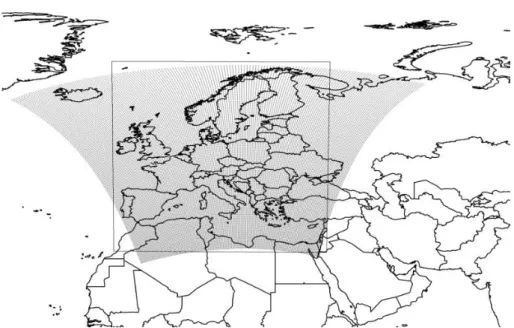
The climate data were obtained from the not bias-corrected regional climate model (RCM) REMO. The horizontal resolution of the grid is 25 km. The model REMO is based on the ECHAM5 global climate model (Roeckner et al., 2003; Roeckner et al., 2004) and the IPCC SRES A1B scenario. The reference period of REMO is 1961-1990, the two future periods of modeling are 2011-2040 and 2041-2070. Although the entire European Continent is within the domain of REMO, we used only a part (25724 of the 32300 points) of the grid shown in Fig. 1. For the distribution modeling, we used 3 × 12 climatic variables: monthly mean temperature (Tmean, °C), monthly minimum temperature (Tmin, °C), and monthly precipitation (P, mm).
Figure 1. The domain of climate model REMO and its part used in the study
Softwares
We used ESRI ArcGIS 10 software for the preparation, management and editing of spatial and climatic data, modeling and present the model results. The management of climatic data and preparation of the expressions for modeling were assisted by Microsoft Excel 2010 program. PAST statistic analyzer software (Hammer et al., 2001) was used for creating histogram (probability density function) and the cumulative distribution function of the climatic parameters, getting the percentile values of the parameters, and creating some statistical analysis of the model results.
Model calibration
For calibrating our climate envelope model a union distribution of the eight studied Phlebotomus species was created, and the model for this aggregated distribution was run iteratively to investigate the optimal amount of percentiles to left from the climatic values. Cumulative distribution functions were calculated by PAST for the 3 × 12 climatic parameters. During the iterative modeling 0 + 0 to 19 + 19 percentiles were left from the lower and higher values of a certain type of climate parameters (e.g. minimum temperatures), while the other 2 × 12 climatic parameters were fixed at the extreme values (0-0 percentiles were left). In the meanwhile two types of error values were calculated: 1) internal – the ratio of the current distribution segment’s area not determined by the model, 2) external – the ratio of area outside the current distribution, determined wrongly by the model. The error functions were accumulated, with the same weights divided between the two function, and the point of minimum value was searched.
It was found that the precipitation parameter drew quite different error functions than the temperatures, therefore we ran another iteration to study the difference between the lower and higher part of the precipitation percentiles. We fixed the two extremes of the
minimum and mean temperatures, and left iteratively more percentiles from the minimum of precipitation values while the maximum was fixed, and vice versa.
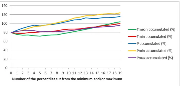
The accumulated error functions (Fig. 2.) showed that leaving percentiles from precipitation and from the minimum of precipitation results in graphs having the minimum point at the origin. Therefore, leaving percentiles from the minimum of precipitation values gives worse model than without percentile leaving. According to the result of iterations, 5-5 percentiles are to left from the two extremes of mean temperature, 2-2 from the two extremes of minimum temperature, and 0 from the minimum and 8 from the maximum of precipitation. Although Cohen’s kappa measurement (Cohen, 1960) is another way of model calibration, final Cohen’s kappa value of our model was calculated (0.54). For further error-based model calibration methods see Fielding and Bell (1997).This result was used during the modeling of Phlebotomus species. Thus the model results are highly comparable with each other, but the models are not really sensitive to the characteristic of certain distributions.
Figure 2. Accumulated errors of modeling while leaving percentiles from the minimum and maximum of mean temperature (Tmean), minimum temperature (Tmin), precipitation (P); from
the minimum of precipitation (Pmin) and from the maximum of precipitation (Pmax)
Modeling method
Before we ran our model on the distribution of Phlebotomus spp., the climatic data were refined by Inverse Distance Weighted interpolation method. Then the modeling steps were as follows in case of certain species: 1) we queried the grid points within the distribution (a few thousand × 36 data) with ArcGIS; 2) the percentile points of the 36 climatic parameters (101 × 36 data) were calculated by PAST; 3) we selected the appropriate percentiles of the climatic parameters mentioned above (2 × 36 data); 4) modeling phrases (3 strings) were created by string functions of Excel for the three modeling periods, 5) the areas were selected where all the climatic values of the certain period were between the extremes selected in step 3. This last step was achieved by Raster Calculator function of ArcGIS. Similar approach was made by Bede-Fazekas (2012).
Length of the active period
The length of the period of activity is one of the most important determinants of the transmission of a parasites to humans, and therefore of the prevalence. According to previous studies about temperature thresholds of their activity [P. neglectus: 13 °C mean temperature (Lindgren and Naucke, 2006); P. papatasi: 16 °C minimum temperature (Colacicco-Mayhugh et al., 2010); P. perniciosus: 15 °C mean temperature (Casimiro et al., 2006)] we counted the number of suitable months in the reference period and the future periods in some locations. All the selected locations are within the current distribution of the certain species.
Comparison of the model results
The ten model results for the reference period based on the distribution of L.
infantum (LEI), the Phlebotomus species (PAR, PNE, PPA, PPF, PPN, PSE, PSI, PTO), and the union distribution of the last ones (PUN, mentioned hereinafter as a stand-alone species) were compared by statistical methods. The input data of the analysis were formatted as a matrix where the rows were bound to species, and the columns meant types of presence-absence. The positive values in the columns expressed the number of grid points of a certain type of presence-absence in case of the species can be found on that location, zero values were displayed in case of the species absent from that point.
The analyses, primarily, are to display the resemblances and differences of the model results but secondarily they can inform about the relations of the current distributions, the environmental demands, and the ecological tolerances of the species.
Firstly Cluster Analysis was applied using paired group algorithm (Unweighted Pair Group Method with Arithmetic Mean, UPGMA; Sokal and Michenel, 1958) and Euclidean similarity measure. After the clustering, Non-metric Multidimensional Scaling (NMDS; Shepard, 1962, Kruskal, 1964) plot was created with Euclidean similarity measure. Finally, PCA (Pearson, 1901, Hotelling, 1933) biplot (Gabriel, 1971) was created. PCA finds hypothetical variables (components) accounting for the variance in the multivariate data as much as possible (Davis, 1986; Harper, 1999). The components are the linear combination of the input variables.
Results
Recent and projected distributions Result maps
The model results are shown in Fig. 3. The climatic thresholds used in the modeling are enumerated in Appendix Table 1.
Figure 3. Current distribution (dark green), modeled potential distribution in the reference period (light green), and predicted potential distribution in the period of 2011-2040 (orange)
and 2041-2070 (yellow) of the eight studied Phlebotomus species
P. ariasi
The currently observed northern limit of P. ariasi’s distribution is near the 49°N latitude, but the area is mainly restricted to Spain and Southern France. Our model shows that the possible range is much wider, it reaches the 53°N latitude in Germany and in the UK. While the northern segment of the potential distribution expands to the German-Polish border (15°E), the southern segment contains almost the entire Balkan Peninsula and the Carpathian Basin, and in addition it includes, the whole Apennine Peninsula without Sicily. Beside the UK, Hungary and Turkey, the major expansion from the potential current distribution can be observed in Germany (2011-2040), and in Poland, Bohemia, Slovakia, Romania, Moldova and Ukraine (2041-2070). P. ariasi is expected to reach the northernmost territories amongst the studied species: Denmark, Sweden, and Norway (59°30’N) are able to be affected in the far future period.
P. perniciosus
Although the present distribution of P. perniciosus is very similar to that of P. ariasi, moreover, the distribution of P. ariasi is slightly smaller, P. perniciosus seems to be less tolerant to the combination of cold summers and lowest winter temperatures than P.
ariasi, since the modeled potential distribution of the former one is remarkably smaller, mainly in West Europe. Similarities can be seen in the projected suitable areas of these species for both the near and far future period, however Germany, Poland, and Bohemia are not as highly affected as in case of P. ariasi. In contrast, in Southeastern Europe the modeled potential distributions both for the reference period and for the future periods have very similar shape in case of the two species. According to the results P.
perniciosus will, as currently, still favor the low-altitude areas. Major expansion is expected in the UK, Germany, Hungary, Romania, Ukraine and Turkey.
P. sergenti and P. similis
P. sergenti and P. similis are typical Mediterranean sandflies, the difference in their current distribution is that P. similis is restricted to the Eastern Mediterranean.
According to our model, their suitable areas are highly overlapped in the reference period and in the future periods too. However, the modeled distributions of P. sergenti are, in all of the periods, slightly larger. By 2070, besides the mainly affected countries (Spain, Italy, Macedonia, Greece and Turkey), Portugal, Albania, Romania, and Ukraine is expected to offer suitable climatic conditions for these two species.
P. neglectus, P. papatasi, P. perfiliewi and P. tobbi
The current distribution, and therefore the environmental demand and the modeled distributions of these four species are similar, the distribution of P neglectus and P.
perfiliewi is almost the same. The latter ones are, in contrast of P. papatasi, absent from Spain, while P. tobbi is definitely restricted to the East Mediterranean. According to the modeled potential distribution in the reference period, all of these sand fly species could inhabit the Carpathian Basin, the Rumanian Lowland, the Balkans, Turkey and the Iberian and Apennine Peninsula. Most of all, P. papatasi has occupied its potential area.
Great northward expansion is not expected in case of these four species, only in France, Hungary and Ukraine.
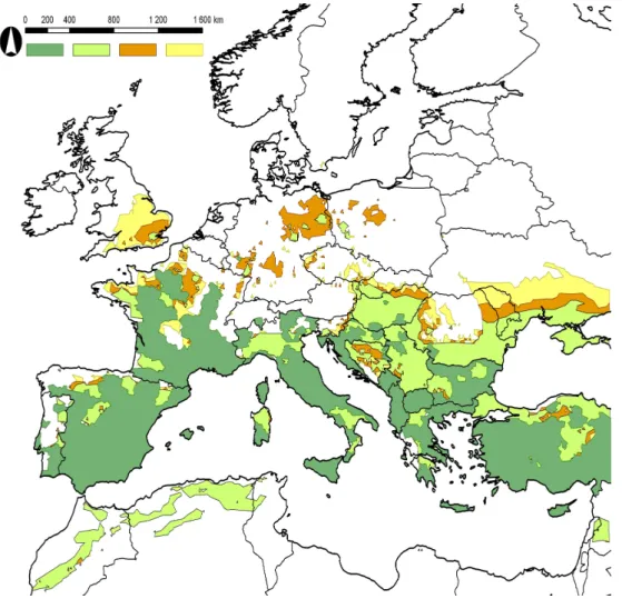
The aggregated distribution of Phlebotomus species
In the case of certain species the mean latitudes that limits their northward future expansion are as follows: 56°N – P. ariasi, 54°N – P. perniciosus, 48°N – P. neglectus, P. papatasi, P. perfiliewi, and P. tobbi, 46°N – L. infantum, and 44°N – P. sergenti, and P. similis. After examining the various Phlebotomus species we evaluate the model result based on the aggregated distribution of them (Fig. 4). According to the differences between the aggregated current distribution of the Phlebotomus species and the modeled potential distribution of this group, the Po River Valley, Serbia, Hungary, the northern Rumanian Lowland, and the coastline of the Black Sea seem to be unsaturated with sand flies recently, while in the western European areas the resident sand flies almost completely fill their potentially suitable areas. The future northern expansion is expected in Britain, Germany, Poland, Bohemia, Slovakia, Hungary, Romania, Moldova and Southern Ukraine (from 47°N to 49°N). The major expansion in the next 30 years can be seen in Germany, however in this country and in Poland expansion in the far future period is not predicted. In the period of 2041-2070 the major expansion is modeled in the UK and north to the Black Sea.
Figure 4. Current distribution (dark green), modeled potential distribution in the reference period (light green), and predicted potential distribution in the period of 2011-2040 (orange)
and 2041-2070 (yellow) of the aggregation of the studied Phlebotomus species
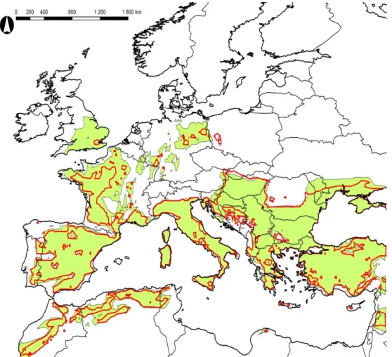
A model validation was applied by comparing, for the reference period, 1) the model result based on the aggregated distribution, and 2) the union of the model result based on separate distributions (Fig 5.). The area of the aggregated model results is slightly larger, but the difference can be seen mainly in territories that were predicted as expansion of the aggregated species in the near future period (UK, France, Germany, Moldova and Ukraine). An opposite type of overlapping is to be observed in Poland, Southern Slovakia, and Northern Hungary. We argue that the model was highly verified by this comparison.
Figure 5. The model result based on the aggregated distribution of the eight Phlebotomus species (red contour) and the aggregated model results based on the individual distributions
(green region). The model was run on the reference period (1961-1990)
Length of the active period
Our model resulted prolongation of the potentially active period. In case of P.
neglectus the number of months is 8, 8 and 9 in Athen, Greece, and 5, 6, and 6 in Pécs, Hungary in the period of 1961-1990, 2011-2040, 2041-2070, respectively. In case of P.
papatasi the number of months is 4, 4 and 6 in Athen, Greece, and 2, 3 and 4 in Szeged, Hungary in the studied three periods. In case of P. perniciosus the number of months is 7, 8 and 8 in Málaga, Spain in the studied three periods, but no prolongation was found in Hungary in monthly resolution.
Discussion
Evaluation of the model
Opinions differ if climate is by itself sufficient or even the most important factor for explaining species distributions (Dormann, 2007). According to Kennewick et al.
(2010) the most important limit of the distribution of sandflies is the winter average and minimum temperatures and the cold and rainy summers. Note, that absolute climatic values and extremes rather than averages may explain the limits of distribution better (Kovács-Láng et al., 2008).
The modeled potential area in the reference period, if there isn’t a major geographical barrier between the inhabited and the unpopulated areas, is greater than the observed one. This difference is clearly visible in the case of P. ariasi in France, in the case of the P. neglectus, P. papatasi, P. perfiliewi and P. tobbi in the Carpathian Basin and in the Southwestern countries of the Balkan Peninsula. A model likely overestimates the possible habitat of a species, but leaving percentiles of the limiting climate values can slightly reduce the overestimation. The modeled and observed distributions are similar in case of P. papatasi, P. sergenti, and P-perniciosus in the western Mediterranean Basin, and P. similisin the eastern Mediterranean Basin.
The goodness of our model was somewhat validated by that the Atlas Mountain was displayed by the model in case of nearly all of the species. Nonetheless, the fact that current distribution data of Africa were not considered by the model can cause problems in observation of the shift in the southern areas of Europe (trailing edge). The modeled retraction in Southwest Spain, coastal parts of South Italy and Greece, and Southwest Turkey is thought to be the blunder of the model. The significant retraction in the Atlas Mountain can, however, be real result.
About modeling vectorial diseases see Peterson (2006). Genetic algorithm, such as GARP program, was used for modeling the distribution of leishmaniasis (Nieto et al., 2006), sandflies (Peterson and Shaw, 2003, Peterson et al., 2004), and other species (Gómez-Mendoza, 2007). There are programs for CEM, such as MaxEnt (Phillips et al., 2006), BioClim (Busby, 1986; Nix, 1986), and Domain (Carpenter et al., 1993). From among them MaxEnt was used for studying sandflies in North America (González et al., 2010), Europe (Chamaillé et. al., 2010), Middle East (Colacicco-Mayhugh et al., 2010), but still for studying Asian tiger mosquito (Medley, 2010) and other insects (Strange et al., 2011; Bidinger et al., 2012).
Comparison of the model results
The first statistical method we used for comparing the model results was Cluster Analysis. The cophenetic correlation coefficient (Sokal and Rohlf, 1962) value of the result was 0.958 (Fig. 6).
100 73
45
39 66
54 56
43 83
0 1,2 2,4 3,6 4,8 6 7,2 8,4 9,6 10,8
800 720 640 560 480 400 320 240 160 80
Distance PUN PPN PNE PPA PPF PTO PSE PSI LEI PAR
Figure 6. The result of the Cluster Analysis based on the presence-absence data with bootstrap values. Paired group method with Euclidean similarity measure was used. Abbreviations: LEI – L. infantum, PAR – P. ariasi, PNE – P. neglectus, PPA – P. papatasi, PPF – P. perfiliewi, PPN – P. perniciosus, PSE – P. sergenti, PSI – P. similis, PTO – P. tobbi, PUN – union distribution
of Phlebotomus
According to the analysis, P. ariasi is the sister group of the major complex of the other nine species with bootstrap value 73 (the clustering was repeated 100 times). The most obvious group was formed by P. similis and P. sergenti with bootstrap value 83. It should be mentioned, that only these two species among the studied ones belong to subgenus Paraphlebotomus according to the conventional, but not proven (Alten, 2010) division of the genera (Lewis, 1982). The complex of the union distribution and P.
pernciosus is, however, not so strong (bootstrap: 45), neither the place of L. infantum (bootstrap: 43).
The NMDS result is related to the aforementioned results. The Shepard plot shows good linearity, and the stress is only 0.01785, which indicates that there was a very little information loss during the dimension reduction in terms of the paired distances.
The Cluster Analysis put L. infantum next to the group of P. sergentiand P. similis in the tree, which result is highly verified by the NMDS. In contrast, there is no evidence, that species of subgenus Paraphlebotomus are vectors of L. infantum, rather they are bound to parasite L. tropica (Ready, 2000; Kamhawi et al., 2000; Depaquitet al., 2002).
The distance of L. infantum and the aggregated Phlebotomus species is the greatest in the major complex. This may be the consequent of the fusion, because the unionedsandfly species contains the whole spectrum of the environmental tolerance of the eight species, and the present endemic areas of L. infantum are located in the
relatively warm, southern part of Europe incorporating the distribution of P. sergentiand P. similis.
The cluster of P. perfiliewi, P. tobbi, P. neglectus, and P. papatasi was proved by the NMDS. Since the NMDS is good statistical method to ordinate the distances of the species, it is obvious that the larger distance from P. ariasi can be seen in case of the cluster of the four species mentioned above and the cluster of P. sergentiand P. similis.
P. perniciosus and the cluster of four species are situated the nearest to the origin. The nearer the place is to the origin, the less summarized difference has from the others.
B A
F E C
D
PAR PUN
PNE PPA
PPF
PPN
PSE PSI
PTO
LEI
-300 -200 -100 100 200 300 400 500 600
-300 -250 -200 -150 -100 -50 50 100 150
Figure 7. The biplot result of the principal component analysis (PCA). Abbreviations: LEI – L.
infantum, PAR – P. ariasi, PNE – P. neglectus, PPA – P. papatasi, PPF – P. perfiliewi, PPN – P. perniciosus, PSE – P. sergenti, PSI – P. similis, PTO – P. tobbi, PUN – union distribution of
Phlebotomus
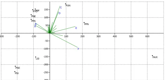
The result of the PCA can be seen on Fig. 7. The six major distinguishing variables were displayed in a map (Fig. 8). The results are confirmed, since the plane stretched by the first and second components are responsible for the 72.08 % of the variance, and only the first four components can explain more than 3% of the variance.
The result of PCA proved the former statistical conclusions. According to the biplot and the map displaying the six major variables it can be stated that 1) the cluster of L.
infantum, P. sergenti, and P. similis is segregated from the others mainly by the common absences of the three species; 2) the aggregated distribution is in the direction of the vector sum of variable as it was expected; 3) the variables C and D are reliable for the presence of the aggregated distribution and for the absence of cluster of L.
infantum. These variables are bound mainly to the northern Mediterranean territories of Europe. They are adjacent to each other and include Northern Spain, Central Italy, Southern Hungary, Serbia, Albania, Macedonia, and Eastern Bulgaria; 4) the large distance of P. papatasi’s cluster and P. ariasi is explained by variables A and B (absence of P. ariasi, presence of the cluster of four), and variable F (presence of P.
ariasi, absence of the cluster of four); 5) variables A and B can be seen in the southern Mediterranean territories of Europe and in the western part of North Africa, including
Southern Spain, Southern Italy, Greece, Western Turkey, Northern Morocco, and Northern Algeria.
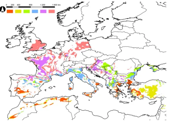
Figure 8. The area of the major distinguishing variables of the biplot PCA. A- orange, B- yellow, C-green, D-blue, E-purple, F-pink
Note, that the difference of the modeled and current distributions is mainly caused by the European input maps of our research. The principal difference is that variable B is displayed at Central Turkey, while the focal point of variable A is western than of variable B; 6) variable E is the most reliable of all for the presence of P. perniciosus, and is neighbor of variable F in the map. They can be found mainly in the Atlantic climate (Southern Britain, France, Germany) and in Western Hungary, Slovenia, Croatia and Bosnia and Herzegovina.
Comparison of our results to the literature
The length and the average temperature of the warm season are important factors (Oshaghi et al., 2009). Our model finds, in contrast the results of Fischer et al. (2011a), that the Benelux States may not be suitable for Phlebotomus species, because they don’t favor the short, relatively cold and rainy summers (Kennewick et al., 2010). Fischer et al. (2011a) expected no migration from southeastern direction, which is strengthened by our results. We found that to the end of the 2060’s the expansion of P. ariasi and P.
perniciosus to Central Europe is most likely among the studied species. The range of suitable areas differs between the two species, which is consistent with Fischer et al.
(2011b). In contrast of Fischer et al. (2011b) we found that to the end of the 2060’s Central and Western Europe will be only suitable for P. ariasi and P. perniciosus, and not for P. perfiliewi and P. neglectus.
The long-distance transport and travelling can play a very important role (Walther et al., 2009), as can be shown in the case of the migrant workers and pets (Neghina et al., 2009). Therefore the modeled discrete potential distributions may be inhabited by the vectors without assuming continuous migration routes.
Conclusion
Each of the selected eight sandfly species showed territorial expansion according to the REMO model, but the size of their potentially inhabited area increase can be very different in various species. Our results are consistent with the literature in the sense that the Central European climate will become more and more suitable especially for P.
ariasi and P. perniciosus, the species whose distribution focuses on the southwestern territories most of all. In the case of the Carpathian Basin six from the studied eight species are projected to potentially present to the end of the 2060’s.
Acknowledgement. The research was supported by Project TÁMOP-4.2.1/B-09/1/KMR-2010-0005 and John Bolyai Research Scholarship of Hungarian Academy of Sciences. The ENSEMBLES data used in this work was funded by the EU FP6 Integrated Project ENSEMBLES (Contract number 505539) whose support is gratefully acknowledged.
REFERENCES
[1] Alten, B. (2010): Historical phlebotomine data for Europe. – "European Network for Arthropod Vector Surveillance for Human Public Health" AGM Antwerp. Conference matter.
[2] Aspöck, H., Gerersdorfer, T., Formayer, H, Walochnik, J. (2008): Sand flies and sandfly-borne infections of humans in Central Europe in the light of climate change. – Wiener klinische Wochenschrift 120(4): 24-29.
[3] Bede-Fazekas, Á. (2012): Methods of modelling the future shift of the so called Moesz- line. – Applied Ecology and Environmental Research 10(2): 141-156.
[4] Belen, A., Alten, B. (2011): Altitudinal variation in morphometric and molecular characteristics of Phlebotomus papatasi populations. – J Vector Ecol Suppl. 1: 87-94.
[5] Bidinger, K., Lötters, S., Rödder, D., Veith, M. (2012): Species distribution models for the alien invasive Asian Harlequin ladybird (Harmonia axyridis). – Journal of Applied Entomology 136: 109-123.
[6] Bongiorno, G., Habluetzel, A., Khoury, C., Maroli, M. (2003): Host preferences of phlebotomine sand flies at a hypoendemic focus of canine leishmaniasis in central Italy.
– Acta Trop 88:109-116.
[7] Bülent, A. (2010): Speciation and Dispersion Hypotheses of Phlebotomine Sand flies of the subgenus ParaPhlebotomus (Diptera:Psychodidae): The Case in Turkey. – Hacettepe J Biol & Chem 38(3): 229-246.
[8] Busby, J.R. (1986): A biogeographical analysis of Nothofagus cunninghamii (Hook.) Oerst. in southeastern Australia. – Aust J Ecol 11: 1-7.
[9] Carpenter, G., Gillison, A.N., Winter, J. (1993): DOMAIN: a flexible modeling procedure for mapping potential distributions of plants, animals. – Biodivers Conserv 2:
667-680.
[10] Casimiro, E., Calheiros, J., Santos, F.D., Kovats, S. (2006): National assessment of human health effects of climate change in Portugal: approach and key findings. – Environ Health Perspect 114(12): 1950-1956.
[11] Chamaillé, L., Tran, A., Meunier, A., Bourdoiseau, G., Ready, P., Dedet, J.P. (2010):
Environmental risk mapping of canine leishmaniasis in France. – Parasites & Vectors 3:
31.
[12] Cohen, J. (1960): A coefficient of agreement for nominal scales. – Educational and Psychological Measurement 20(1): 37-46.
[13] Colacicco-Mayhugh, M.G., Masuoka, P.M., Grieco, J.P. (2010): Ecological niche model of Phlebotomus alexandri and P. papatasi (Diptera: Psychodidae) in the Middle East. – International Journal of Health Geographics 9: 2.
[14] Czúcz, B. (2010): Modelling the impact of climate change on natural habitats in Hungary. – PhD dissertation. Corvinus University of Budapest, Faculty of Horticultural Sciences. Budapest, Hungary.
[15] Davis, J.C. (1986): Statistics and Data Analysis in Geology. – John Wiley & Sons, New York.
[16] De la Roque, S., Rioux, J.A. Slingenbergh, J. (2008): Climate change: Effects on animal disease systems and implications for surveillance and control. – Revue Scientifique Et Technique. International Des Epizooties 27(3): 39-54.
[17] Depaquit, J., Ferté, H., Léger, N., Lefranc, F., Alves-Pires, C., Hanafi, H., Maroli, M., Morillas-Marquez, F., Rioux, J.A., Svobodova, M., Volf, P. (2002): ITS 2 sequences heterogeneity in Phlebotomus sergenti and Phlebotomus similis (Diptera, Psychodidae):
possible consequences in their ability to transmit Leishmania tropica. – International Journal for Parasitology 32(9): 1123-1131.
[18] Dormann, C.F., (2007): Promising the future? Global change projections of species distributions. – Basic and Applied Ecology 8: 387-397.
[19] Elith, J., Leathwick, J.R. (2009): Species Distribution Models: Ecological Explanation and Prediction Across Space and Time. – Annual Review of Ecology, Evolution and Systematics 40(1): 677-697.
[20] ENSEMBLES data archive (2012): ensemblesrt3.dmi.dk. – Last accessed: 2012.11.01.
[21] Farkas, R., Tánczos, B., Bongiorno, G., Maroli, M., Dereure, J., Ready, P.D. (2011):
First surveys to investigate the presence of canine leishmaniasis and its phlebotomine vectors in Hungary. – Vector Borne Zoonotic Dis 11: 823-34.
[22] Ferroglio, E., Maroli, M., Gastaldo, S., Mignone, W., Rossi, L. (2005): Canine leishmaniasis, Italy. – Emerg Infect Dis 11: 1618-1620.
[23] Fielding, A.H., Bell, J.F. (1997): A review of methods for the assessment of prediction errors in conservation presence/absence models. – Environmental Conservation 24(1):
38-49.
[24] Fischer, D., Thomas, S.M., Beierkuhnlein, C. (2011b): Modelling climatic suitability and dispersal for disease vectors: the example of a phlebotomine sandfly in Europe. – Procedia Environmental Sciences 7: 164-169.
[25] Fischer, D., Moeller, P., Thomas, S.M., Naucke, T.J., Beierkuhnlein, C. (2011a):
Combining climatic projections and dispersal ability: a method for estimating the responses of sandfly vector species to climate change. – PLoS Negl Trop Dis 11: e1407.
[26] Fischer, D., Thomas, S.M., Beierkuhnlein, C. (2010): Temperature-derived potential for the establishment of phlebotomine sand flies and visceral leishmaniasis in Germany. – Geospatial Health 5(1): 59-69.
[27] Gabriel, K.R. (1971): The biplot graphic display of matrices with application to principal component analysis. – Biometrika 58(3): 453–467.
[28] GISCO – Eurostat (European Commission) (2012): epp.eurostat.ec.europa.eu/portal/
page/portal/gisco_Geographical_information_maps/popups/references/administrative_u nits_statistical_units_1. Last accessed: 2012.11.21.
[29] Gómez-Mendoza, L., Arriaga, L. (2007): Modeling the effect of climate change on the distribution of oak and pine species of Mexico. – Conservation Biolog 21: 1545-1555.
[30] González C., Wang, O., Strutz, S.E., González-Salazar, C., Sánchez-Cordero, V., Sarkar, S. (2010): Climate change and risk of leishmaniasis in North America:
predictions from ecological niche models of vector and reservoir species. – PLoS Negl Trop Dis 19(4): 585.
[31] Guisan, A., Zimmermann, N.E. (2000): Predictive habitat distribution models in ecology. – Ecological Modelling 135(2-3): 147-186.
[32] Hammer, Ř., Harper, D.A.T., Ryan, P.D. (2001): PAST: Paleontological statistics software package for education and data analysis. – Palaeontologia Electronica 4(1): 9.
[33] Harper, D.A.T. (ed.). (1999): Numerical Palaeobiology. – John Wiley & Sons, Chichester.
[34] Hijmans, R.J., Graham, C.H. (2006): The ability of climate envelope models to predict the effect of climate change on species distributions. – Global Change Biology 12:
2272-2281.
[35] Hotelling, H. (1933): Analysis of a Complex of Statistical Variables Into Principal Components. – Journal of Educational Psychology 24: 417-441, 498-520.
[36] Ibánez, I., Clark, J.S., Dietze, M.C., Feeley, K., Hersh, M., Ladeau, S., Mcbride, A., Welch, N.E., Wolosin, M.S. (2006): Predicting Biodiversity Change: Outside the Climate Envelope, beyond the Species-Area Curve. – Ecology 87(8): 1896-1906.
[37] Kamhawi, S., Modi, G.B., Pimenta, P.F., Rowton, E., Sacks, D.L. (2000): The vectorial competence of Phlebotomus sergenti is specific for Leishmania tropica and is controlled by species-specific, lipophosphoglycan-mediated midgut attachment. – Parasitology 121(Pt1): 25-33.
[38] Kennewick, W., Anthony, A., Marfin, A. (2010): Emerging Vector-Borne Infectious Diseases What's New in Medicine – Workshop.
[39] Killick-Kendrick, R. (1990): Phlebotomine vectors of the leishmaniases: a review. – Medical and Veterinary Entomolog 4: 1-24.
[40] Kocsis, M., Hufnagel, L. (2011): Impacts of climate change on Lepidoptera species and communities. – Applied Ecology and Environmental Research 9:43-72.
[41] Köhler, K., Stechele, M., Hetzel, U., Domingo, M., Schönian, G., Zahner, H., Burkhardt, E. (2002): Cutaneous leishmaniosis in a horse in southern Germany caused by Leishmania infantum. – Vet Parasitol 16(109): 9-17.
[42] Kovács-Láng, E., Kröel-Dulay, Gy., Czúcz, B. (2008): Az éghajlatváltozás hatásai a természetes élővilágra és teendőink a megőrzés és kutatás területén. – Természetvédelmi Közlemények 14: 5-39.
[43] Kruskal, J.B. (1964): Multidimensional scaling by optimizing goodness of fit to a nonmetric hypothesis. – Psychometrika 29: 1-28.
[44] Ladányi, M., Horváth, L. (2010): A review of the potential climate change impact on insect populations – general and agricultural aspects. – Appl Ecol Environ Res 8: 143- 152.
[45] Léger, N., Depaquit, J., Ferté, H., Rioux, J.A., Gantier, J.C., Gramiccia, M., Ludovisi, A., Michaelides, A., Christophi, N., Economides, P. (2000): Phlebotomine sand flies (Diptera: Psychodidae) of the isle of Cyprus. II – isolation and typing of Leishmania (Leishmania infantum Nicolle, 1908 (zymodeme MOM 1) from Phlebotomus (Larrouius) tobbi Adler and Theodor, 1930. – Parasite 7: 143-146.
[46] Lewis, D.J. (1982): A taxonomic review of the genus Phlebotomus (Diptera:
Psychodidae). – Bulletin of the British Museum Natural History (Entomology Series) 45(2): 121-209.
[47] Lindgren, E., Naucke, T. (2006): Leishmaniasis: Influences of Climate and Climate Change Epidemiology, Ecology and Adaptation Measures. In. B. Menne and K. L. Ebi (eds.), Climate change and adaptation strategies for human health. – Steinkopff Verlag, Darmstadt. pp 131-156.
[48] Maroli, M., Rossi, L., Baldelli, R., Capelli, G., Ferroglio, E., Genchi, C., Gramiccia, M., Mortarino, M., Pietrobelli, M., Gradoni, L. (2008): The northward spread of leishmaniasis in Italy: evidence from retrospective and ongoing studies on the canine reservoir and phlebotomine vectors. – Trop Med Int Health 13: 256-264.
[49] Maroli, M., Gramiccia, M., Gradon., L., Ready, P.D., Smit, D.F., Aquino, C. (1988):
Natural infections of phlebotomine sand flies with Trypanosomatidae in central and south Italy. – Trans R Soc Trop Med Hyg 82: 227-228.
[50] Medley, K.A. (2010): Niche shifts during the global invasion of the Asian tiger mosquito, Aedes albopictus Skuse (Culicidae), revealed by reciprocal distribution models. – Global Ecology and Biogeography 19: 122-133.
[51] Mencke, N. (2011): The importance of canine leishmaniosis in non-endemic areas, with special emphasis on the situation in Germany. – Berl Munch Tierarztl Wochenschr 124:
434-42.
[52] Minter, D.M. (1989): The leishmaniasis. In: Geographical distribution of arthropod- borne diseases and their principal vectors. – WHO, Geneva (document WHO/VBC/89.967).
[53] Naderer, T., Ellis, M.A., Sernee, M.F., De Souza, D.P., Curtis, J., Handman, E., McConville, M.J. (2006): Virulence of Leishmania major in macrophages and mice requires the gluconeogenic enzyme fructose-1,6-bisphosphatase. – PNAS 103(14):
5502-5507.
[54] Naucke, T.J. (2002): Leishmaniosis, a tropical disease and its vectors (Diptera Psychodidae, Phlebotominae) in Central Europe. – Denisia 6: 163-178.
[55] Neghina, R., Neghina, A.M., Merkler, C., Marincu, I., Moldovan, R., Iacobiciu, I.
(2009): Importation of visceral leishmaniasis in returning Romanian workers from Spain.). – Travel Med Infect Dis 7: 35-39.
[56] Nieto, P., Malone, J.B., Bavia, M.E. (2006): Ecological niche modeling for visceral leishmaniasis in the state of Bahia, Brazil, using genetic algorithm for rule-set prediction and growing degree day-water budget analysis. – Geospatial Health 1: 115- 126.
[57] Nix, H. (1986): A biogeographic analysis of Australian elapid snakes. Atlas of Elapid Snakes of Australia. – Australian Government Publishing Service, Canberra, Australia.
pp. 4-15.
[58] Oshaghi M.A., Maleki Ravasanb, N., Javadiana, E., Rassia, Y., Sadraeib, J., Enayatic, A.A., Vatandoosta, H., Zarea, Z., Emamia, S.N. (2009): Application of predictive degree day model for field development of sandfly vectors of visceral leishmaniasis in northwest of Iran. – J Vector Borne Dis 46: 247-254.
[59] Pearson, K. (1901): On lines and planes of closest fit to systems of points in space. – Philosophical Magazine 6(11): 559-572.
[60] Peterson, A.T. (2006): Ecological niche modeling and spatial patterns of diseases transmission. – Emerging Infectious Diseases 12: 1822-1826.
[61] Peterson, A.T., Shaw, J. (2003): Lutzomyia vectors for cutaneous leishmaniasis in Southern Brazil: Ecological niche models, predicted geographic distributions, and climate change effects. – International Journal for Parasitoloty 33: 919-931.
[62] Peterson, A.T., Pereira, R.S., Neves, V.F. (2004): Using epidemiological survey data to infer geographic distributions of leishmaniasis vector species. – Revista da Sociedade Brasileira de Medcina Tropical 37: 10-14.
[63] Phillips, S.J., Anderson, R.P., Schapire, R.E. (2006): Maximum entropy modeling of species geographic distributions. – Ecological Modeling 190: 231-259.
[64] Pickett, S.T.A. (1989): Space-for-time substitution as an alternative to long-term studies. In Likens, G.E. (ed.) Long-Term Studies in Ecology: Approaches and Alternatives. – Springer, New York. pp. 110-135.
[65] Postigo, J.A. (2010): Leishmaniasis in the World Health Organization Eastern Mediterranean Region. – International Journal of Antimicrobial Agents 36(Supl.1):
S62-S65.
[66] Ready, P.D. (2000): Sand Fly Evolution and its Relationship to Leishmania Transmission. – Mem Inst Oswaldo Cruz, Rio de Janeiro 95(4): 589-590.
[67] Ready, P.D. (2008): Leishmaniasis emergence and climate change. – Rev Sci Tech 27:
399-412.
[68] Ready, P.D. (2010): Leishmaniasis emergence in Europe. – Euro Surveill 15: 19505.
[69] Rioux, J.A., Aboulker, J.P., Lanotte, G., Killick-Kendrick, R., Martini-Dumas, A.
(1985): Ecology of leishmaniasis in the south of France. 21. Influence of temperature on the development of Leishmania infantum Nicolle, 1908 in Phlebotomus ariasi Tonnoir, 1921. Experimental study. – Ann Parasitol Hum Comp 60: 221-229.
[70] Roeckner E., Bäuml, G., Bonaventura, L., Brokopf, R., Esch, M., Giorgetta, M., Schulzweida, Hagemann, S., Kirchner, I., Kornblueh, L., Manzini, E., Rhodin, A., Schlese, U., Tompkins, U.A. (2003): The atmospheric general circulation model ECHAM 5. Part I: Model description. – Max-Planck-Institut für Meteorologie, Hamburg, Germany.
[71] Roeckner E., Brokopf, R., Esch, M., Giorgetta, M., Hagemann, S., Kornblueh, L., Manzini, E., Schlese, U., Schulzweida, U. (2004): The atmospheric general circulation model ECHAM 5. PART II: Sensitivity of Simulated Climate to Horizontal and Vertical Resolution. – Max-Planck-Institut für Meteorologie, Hamburg, Germany.
[72] Rogers D.J., Randolph, S.E. (2006): Climate Change and Vector-Borne Diseases. – Advances in Parasitology 62: 345-381.
[73] Shaw, S.E., Langton, D.A., Hillman, T.J. (2009): Canine leishmaniosis in the United Kingdom: a zoonotic disease waiting for a vector? – Vet Parasitol 26(163): 281-285.
[74] Shepard, R.N. (1962): The analysis of proximities: Multidimensional scaling with an unknown distance function (parts 1 and 2). – Psychometrika 27: 125-140, 219-249.
[75] Skov, F., Svenning, J.C. (2004): Potential impact of climatic change on the distribution of forest herbs in Europe. – Ecography 27(3): 366-380.
[76] Sokal, R.R., Michener, C.D. (1958): A statistical method for evaluating systematic relationships. – University of Kansas Science Bulletin 28: 1409-1438.
[77] Sokal, R.R., Rohlf, F.J. (1962): The comparison of dendrograms by objective methods.
– Taxon 11: 33-40.
[78] Strange, J.P., Koch, J.B. Gonzalez, V.H., Nemelka, L., Griswold, T. (2011): Global invasion by Anthidium manicatum (Linnaeus) (Hymenoptera: Megachilidae): assessing potential distribution in North America and beyond. – Biological Invasions 13: 2115- 2133.
[79] Tánczos, B., Balogh, N., Király, L., Biksi, I., Szeredi, L., Gyurkovsky, M., Scalone, A., Fiorentino, E., Gramiccia, M., Farkas, R. (2012): First record of autochthonous canine leishmaniasis in Hungary. – Vector Borne Zoonotic Dis 12: 588-594.
[80] VBORNET maps – Sand flies (2012): ecdc.europa.eu/en/activities/diseaseprogrammes/
emerging_and_vector_borne_diseases/pages/vbornet_maps_sandflies.aspx?MasterPage
=1. Last accessed: 2012.11.23.
[81] Walther G.R., Roques, A., Hulme, P.E., Sykes, M.T., Pyšek, P., Kühn, I., Zobel, M., Bacher, S., Botta-Dukát, Z., Bugmann, H., Czúcz, B., Dauber, J., Hickler, T., Jarošík, V., Kenis, M., Klotz, S., Minchin, D.,Moora, M., Nentwig, W., Ott, J., Panov, V.E., Reineking, B., Robinet, C., Semenchenko, V., Solarz, W., Thuiller, W., Vila, M., Vohland, K., Settele, J. (2009): Alien species in a warmer world: risks and opportunities. – Trends in Ecology and Evolution 24(12): 686-693.
[82] WHO (1984): The leishmaniases: report of an expert committee. – WHO Tech Rep Ser 701: 1-140.
Appendix
Table 1. The climatic extrema of the eight Phlebotomus species, their aggregation and the L.
infantum used in the modeling. Abbreviations: LEI – L. infantum, PAR – P. ariasi, PNE – P.
neglectus, PPA – P. papatasi, PPF – P. perfiliewi, PPN – P. perniciosus, PSE – P. sergenti, PSI – P. similis, PTO – P. tobbi, PUN – union distribution of Phlebotomus
month 1 2 3 4 5 6 7 8 9 10 11 12
PUN min(Tmean), °C -1,2 -0,5 2,9 6,3 10,1 14,4 16,7 16,2 13,8 8,9 4,2 -0,3 PUN max(Tmean), °C 10,5 10,8 12,6 14,9 18,8 24,1 27,5 28,1 24,4 19,2 14,7 11,5 PUN min(Tmin), °C -8,4 -7,8 -3,5 0,3 3,5 7 9,1 8,8 6,7 3 -0,6 -6,4 PUN max(Tmin), °C 9,3 9 10,4 12,1 15,1 19,4 23 23,8 21,3 17,1 13,3 10,3
PUN min(P), mm 18 18 15 12 6 0 0 0 0 6 12 18
PUN max(P), mm 180 126 141 132 111 78 75 72 78 123 171 138
PAR min(Tmean), °C -0,6 0,3 2,4 5,3 9 12,9 15,1 14,7 12,4 8,1 3,4 1,2 PAR max(Tmean), °C 9,5 10,1 11,6 13,8 17 22,4 25,6 26,1 22,6 17,6 13 10,4
PAR min(Tmin), °C -8,8 -7,9 -6 -1,8 2,1 5,7 7,6 7,7 5,9 2,8 -2 -5
PAR max(Tmin), °C 8,1 8,3 9,5 10,8 13,6 18,2 20,9 21,7 19,3 15,3 11,3 9,2
PAR min(P), mm 21 21 27 21 15 6 0 3 15 27 30 21
PAR max(P), mm 183 141 159 156 138 96 87 84 93 150 186 156
PNE min(Tmean), °C -2,4 -1,7 2,7 6,8 10,8 15,3 18,5 18,2 14,6 9 4,3 -1,5 PNE max(Tmean), °C 10 10,1 12,3 15,1 19,4 24,6 28,6 29,1 25 19,7 15,2 11,1 PNE min(Tmin), °C -8 -8,2 -3 0,8 3,9 7,5 10,4 10,3 7,3 3,1 -0,1 -6,8 PNE max(Tmin), °C 8,7 8,3 9,8 12,1 15,5 19,9 23,8 24,6 21,9 17,3 13,3 9,8
PNE min(P), mm 24 24 21 15 6 0 0 0 3 9 15 24
PNE max(P), mm 207 144 138 120 78 54 45 45 72 114 189 171
PPA min(Tmean), °C -0,5 0,3 3,8 7,5 11,6 16 18,7 18,8 15,3 9,9 5,3 0,3 PPA max(Tmean), °C 10,7 11,1 13 15,5 19,3 24,6 28,6 29,1 25,3 20 15,3 11,7
PPA min(Tmin), °C -6 -5,6 -1,5 1,7 4,7 8,6 11,3 11,3 8,2 4 1 -4,2
PPA max(Tmin), °C 9,6 9,4 10,8 12,9 15,9 20,2 23,8 24,6 21,9 17,8 14,2 10,8
PPA min(P), mm 18 18 15 12 6 0 0 0 0 6 12 18
PPA max(P), mm 177 120 129 114 81 57 45 42 66 108 162 138
PPF min(Tmean), °C -2,3 -1,3 2 5,8 10 14,5 17,4 16,9 13,6 8,4 3,7 -0,9 PPF max(Tmean), °C 10,5 10,4 12,4 15,4 19,6 24,8 28,8 29,1 25,3 20,2 15,7 11,6 PPF min(Tmin), °C -10 -8,1 -4,7 -0,5 3,1 6,7 8,7 8,2 6,2 2,7 -1,6 -6,4 PPF max(Tmin), °C 9,3 8,8 10,2 12,8 16 20,5 24 24,8 22,1 17,5 14,1 10,4
PPF min(P), mm 18 21 15 12 6 0 0 0 0 6 12 18
PPF max(P), mm 216 147 144 132 90 66 51 57 90 141 216 171
PPN min(Tmean), °C 0,5 1,4 3,4 6,2 9,8 14,1 16,1 15,9 13,6 8,8 4,2 2,1 PPN max(Tmean), °C 10,7 11,2 12,9 14,8 18,4 23,6 26,9 27,4 24,2 19 14,4 11,6 PPN min(Tmin), °C -9,4 -8 -4,7 -0,8 2,8 6,1 8,3 8 5,9 2,7 -1,9 -6,1 PPN max(Tmin), °C 9,4 9 10,4 11,7 14,4 18,7 22,3 23,1 20,8 16,4 12,7 10,3
PPN min(P), mm 18 18 24 18 12 3 0 3 9 18 24 21
PPN max(P), mm 171 117 144 135 117 84 78 81 81 129 171 126
PSE min(Tmean), °C -0,7 0,1 3,9 7,7 11,4 16,3 19,2 19,4 15,7 10,1 5,3 -0,1 PSE max(Tmean), °C 10,8 11,3 13,2 15,7 19,4 24,9 28,8 29,4 25,9 20,2 15,3 11,7 PSE min(Tmin), °C -7,2 -6,4 -1,8 1,7 4,5 8,6 11,4 11,4 8,7 4 0,8 -6,1 PSE max(Tmin), °C 9,4 9,2 10,5 12,8 15,8 20,2 23,9 23,9 21,9 17,5 13,4 10,5
PSE min(P), mm 18 18 15 12 6 0 0 0 0 6 12 18
PSE max(P), mm 183 123 144 114 75 42 27 24 45 93 135 135
PSI min(Tmean), °C -0,1 0,3 4 7,8 11,9 16,8 20,2 20,3 15,7 10,1 5,7 0,4 PSI max(Tmean), °C 10 9,8 11,7 14,7 19 24,4 28,3 28,9 24,3 19,1 14,9 11,2 PSI min(Tmin), °C -4 -4,2 -0,8 2,2 5,3 9,4 12,7 12,8 9,1 4,5 1,3 -3 PSI max(Tmin), °C 8,5 8 9,6 11,8 14,8 19,3 23,1 23,6 20,8 16,3 12,9 9,6
PSI min(P), mm 24 27 21 15 6 0 0 0 3 9 15 24
PSI max(P), mm 180 120 114 93 60 36 27 24 36 69 129 150
PTO min(Tmean), °C -2,7 -1,8 2,5 6,5 10,6 15,1 18,3 18,1 14,3 8,9 4,2 -1,9 PTO max(Tmean), °C 10,2 10,2 12,8 16,2 20 25,3 29,2 29,7 26,3 20,9 15,9 11,3
PTO min(Tmin), °C -8 -8 -2,8 0,8 4 7,6 10,6 10,5 7,4 3,2 0 -6,7
PTO max(Tmin), °C 9 8,5 10,2 13 16,5 20,8 24,3 25 22,3 17,8 14,1 10,3
PTO min(P), mm 18 21 15 12 6 0 0 0 0 6 12 18
PTO max(P), mm 216 150 141 120 78 66 51 51 69 114 192 174
LEI min(Tmean), °C 1,9 2,7 4,8 7,5 11,8 16,5 19,4 19,6 16,1 11 6,1 3,3 LEI max(Tmean), °C 11,1 11,3 12,9 15 18,8 23,8 27 27,2 23,8 19,1 14,9 12,2
LEI min(Tmin), °C -2 -1,6 0,2 2,1 4,9 9,1 11,6 12 9,4 5,3 2 -0,4
LEI max(Tmin), °C 9,5 9,2 10,5 12,1 14,8 19,1 22,3 23 20,3 16,9 13,6 10,7
LEI min(P), mm 18 18 21 15 6 0 0 0 3 9 18 21
LEI max(P), mm 183 111 147 120 84 48 39 36 72 120 171 123