Nutation in antiferromagnetic resonance Ritwik Mondal,

(1)

Ritwik Mondal,^∗ Sebastian Großenbach, Levente Rózsa, and Ulrich Nowak Fachbereich Physik, Universität Konstanz, DE-78457 Konstanz, Germany

(Dated: April 16, 2021)

The effect of inertial spin dynamics is compared between ferromagnetic, antiferromagnetic and ferrimagnetic systems. The linear response to an oscillating external magnetic field is calculated within the framework of the inertial Landau–Lifshitz–Gilbert equation using analytical theory and computer simulations. Precession and nutation resonance peaks are identified, and it is demonstrated that the precession frequencies are reduced by the spin inertia, while the lifetime of the excitations is enhanced. The interplay between precession and nutation is found to be the most prominent in antiferromagnets, where the timescale of the exchange-driven sublattice dynamics is comparable to inertial relaxation times. Consequently, antiferromagnetic resonance techniques should be better suited for the search for intrinsic inertial spin dynamics on ultrafast timescales than ferromagnetic resonance.

I. INTRODUCTION

Deterministic spin switching at ultrashort timescales builds the fundament for future spin-based memory tech- nology [1–5]. At femtosecond timescales inertial switching becomes particularly relevant, where the reversal is achieved with a linear momentum gained by the interaction of an ultrashort pulse and spin inertia [6, 7]. The understanding of magnetic inertia has been pursued along two different directions so far.

On the one hand, spin dynamics in antiferromagnets (AFMs) and ferrimagnets (FiMs) has successfully been described by the Landau–Lifshitz–Gilbert (LLG) equation [8–

10] for two sublattices coupled by the exchange interaction.

The exchange energy created by tilting the sublattice magnetization directions away from the antiferromagnetic ori- entation is dynamically transformed into anisotropy energy by collectively rotating the sublattices away from the easy magnetic direction [11], analogously to the transition between kinetic and potential energy terms in a harmonic oscillator. While the LLG equation for the two sublattices is of first order in time, this effect gives rise to an ef- fectively inertial second-order differential equation for the order parameter in AFMs [12, 13]. The interaction between exchange and anisotropy degrees of freedom causes an exchange enhancement of AFM resonance frequencies and linewidths [14].

On the other hand, an intrinsic inertia also arises in magnetic systems, if it is assumed that the directions of spin angular and magnetic moments become separated in the ultrafast dynamical regime [15, 16]. The inertia gives rise to spin nutation, a rotation of the magnetization around the angular momentum direction [17], caused by the energy transfer between magnetic kinetic and potential energy terms. The emergence of spin inertia has been explained based on an extension of the breathing Fermi surface model [18, 19], calculated from a s−d like interaction between the magnetization density and electron spin [20] and derived from a fundamental relativistic Dirac theory [21,22].

Magnetic inertia can be associated with a torque term containing a second-order time derivative of the magnetic moment appearing in the inertial LLG (ILLG) dynamical

∗ritwik.mondal@uni-konstanz.de

equation. The characteristic inertial relaxation time, using its definition in Eq. (1) below, is expected to range from 1 fs [15, 20,23,24] to a few hundred fs [25].

Linear-response theory predicted the emergence of a nutation resonance besides the conventional precession resonance in ferromagnets (FMs) [26–28], providing a possible way of detecting inertial dynamics by applying oscillating external fields. An indirect evidence of the inertial dynamics was found in NiFe and Co samples [23] by following the field dependence of the ferromagnetic precession resonance (FMR) peaks. The experimental observation of the nutation resonance has only been achieved very recently in NiFe and CoFeB using intense terahertz magnetic field transients [25].

While the notion of inertial dynamics has been applied both in the context of the LLG equation for AFMs as well as in the ILLG equation for FMs, the linear response of these two examples is fundamentally different. While in both cases a pair of resonances is found in contrast to the single FMR peak, the excitation frequencies in an AFM are degenerate in the absence of a static external field, while they differ by several orders of magnitude in the ILLG equation. The effective damping parameter of the precession, defined as the half-width of the peak at half-maximum, is considerably higher in AFMs than in FMs, where it corresponds to the Gilbert damping. In contrast, it was demonstrated that the effective damping decreases in the ILLG equation applied to FMs [27], particularly at the nutation resonance [29]. However, the ILLG has not been applied to AFMs so far.

Here, we explore the effects of the ILLG equation in two-sublattice AFMs and FiMs using linear-response theory and computer simulations. It is shown that a pair of nutation resonance peaks emerges, and that the inertial relaxation time influences the precessional resonance significantly stronger in AFMs than in FMs due to the exchange coupling between the sublattices. The effective damping parameter is found to decrease in AFMs, reaching considerably lower values than the Gilbert damping at the nutation peak, thereby enhancing the lifetime of these excitations. The inertial effects in FiMs are found to interpolate between those in AFMs and FMs.

II. METHODS

As derived in earlier works [15,21,22], the ILLG equation

arXiv:2012.02790v3 [cond-mat.mtrl-sci] 15 Apr 2021

(2)

reads

M˙_i=−γ_iM_i×H_i+ α_i Mi0

M_i×M˙_i+ η_i Mi0

M_i×M¨_i, (1) generalized here to multiple sublattices indexed byi. The first, second and third terms in Eq. (1) describe spin precession with gyromagnetic ratio γi, transverse relaxation with Gilbert damping αi, and inertial dynamics with relaxation time ηi. Note that an alternative notation for the inertial term with η_i = α_iτ_i is also used in the liter- ature [15, 23, 25]; where comparison with earlier works is mentioned in the following, the relaxation time is converted to the formulation of Eq. (1). The equation of motion was treated analytically as described in the following sections, and also solved numerically using an algorithm presented in detail in AppendixA.

III. INERTIAL EFFECTS IN FERROMAGNETS First, we summarize the effects of the inertial term on FM resonance. The FM is described by the free energy F(M) = −H0Mz−KM_z²/M₀², modeling a single sublattice where spatial modulations of the magnetization are ne- glected. M₀is the magnitude of the magnetic moment,H₀ is the applied external field andKis the uniaxial anisotropy energy, also considered to include demagnetization effects in the form of a shape anisotropy. The effective field can be written asH=−∂F/∂M = (H0+ 2KMz/M₀²) ˆez, and the magnetic moment is oriented along thez direction in equilibrium.

The linear response to a small transversal external field component h(t) is calculated considering M = M0eˆz + m(t) and expanding Eq. (1) up to first order in h(t)and m(t). The exciting field is assumed to be circularly polarized, h_± =h_x±ih_y =he^±iωt, with a similar time dependence for the response, m± = mx±imy = me^±iωt. The calculated susceptibility reads (see AppendixBfor details)

m_±=χ_±h_±= γM0

Ω₀−ω−ηω²±iαωh_±, (2) with Ω0 = γ(H0M0+ 2K)/M0. It is found that the Gilbert damping is associated with the imaginary part of the susceptibility, while the inertial term contributes to the real part of the susceptibility, which is consistent with the previous calculation in Ref. [21]. The dissipated power is calculated asP = ˙m·h= ωIm(χ₊)|h|². We note that a linearly polarized exciting field can be described as a linear combination of circularly polarized fields with ω and −ω frequencies.

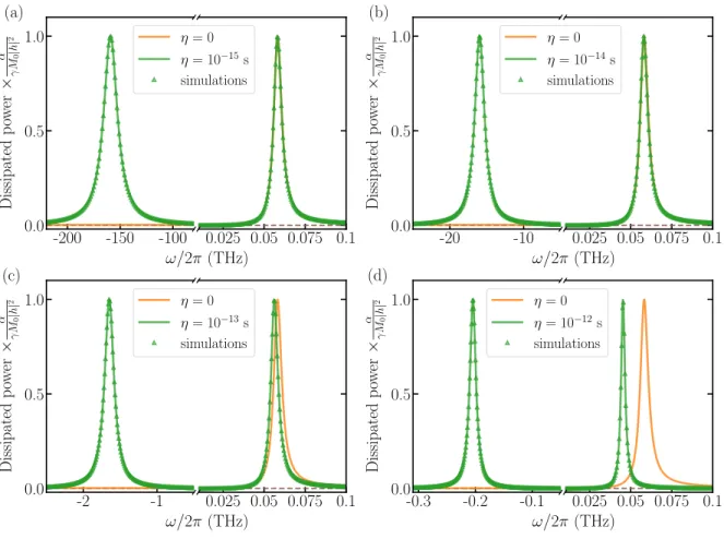
The dissipated power with and without the inertial term is shown in Fig. 1. The data points denoted by symbols in Fig. 1 denote the results of the atomistic spin simulations (see AppendixAfor details). The relaxation time is chosen to range from η = 10⁻¹⁵ s to η = 10⁻¹² s. This covers the fs timescales described in Refs. [20, 23, 24] and

the values of around 300 fs in Ref. [25]. It can be observed that the inertial dynamics reduces the precession resonance frequency. The resonance peak position is well approxi- mated as ωp = √

1 + 4βFM−1

/(2η) ≈ Ω0(1−βFM), with β_FM = ηΩ0. The associated shift in the resonance field H_p was investigated in Ref. [23]. However, note that the relative value of this shift is very low since β_FM 1, meaning that it can only be observed ifΩ0is shifted to high values, for example by a strong external field H0.

The most profound effect of the inertial dynamics is the emergence of a second resonance peak, associated with the spin nutation. Its frequency is approximately ωn =

− √1 + 4β_FM+ 1

/(2η) ≈ −1/η−Ω0(1−β_FM). Simi- larly to the precession frequency, the subleading corrections βFMΩ0 are small. The negative sign of the frequency im- plies an opposite rotational sense [30]: while the precession is excited by a circularly polarized field rotating counter- clockwise, the nutation resonance reveals an opposite polarization.

The effective damping parameter is defined as the ratio of the imaginary and the real parts of the frequency where Eq. (2) has a node, and is approximately expressed as αeff,p =αeff,n ≈α(1−2βFM), see AppendixBfor the derivation. Since the imaginary part characterizes the half- width of the resonance peak at half maximum, the latter suggests that the linewidth of FMR decreases due to the inertia, in agreement with the numerical results in Ref. [27].

The relative value of the reduction is once again governed by the factor βFM.

IV. INERTIAL EFFECTS IN

ANTIFERROMAGNETS AND FERRIMAGNETS

Next, we consider AFMs and FiMs with two sublattices A and B. Assuming once again homogeneous sublattice magnetizations, the free energy is expressed as

F(M_A,M_B) =−H₀(M_Az+M_Bz)

− KA

M_A0² M_Az² − KB

M_B0² M_Bz² + J MA0MB0

MA·MB, (3) with the external field applied along the z direction, H₀ = H₀eˆ_z, uniaxial easy-axis anisotropy con- stants KA, KB and intersublattice exchange coupling J. From the free energy, the associated fields entering the sublattice ILLG equations (1) can be determined using H_A/B = −∂F(MA,MB)/∂M_A/B = H0eˆz + 2K_A/BM_A/Bz/M_A/B0² eˆz−JM_B/A/(MA0MB0). In equilibrium, the sublattice magnetizations are aligned antiparallel along thezdirection. Linear response to the transverse homogeneous external field hA(t) =hB(t)may be calculated similarly to the FM case, using the expansions MA(r, t) = MA0eˆz+mA(t)andMB(r, t) =−MB0eˆz+mB(t).

The two-sublattice susceptibility tensor is expressed as follows (see Appendix Cfor details):

m_A±

m_B±

=χ^AB_± h_A±

h_B±

= 1

∆_± 1

γ_BM_B0 ΩB±iωαB−ηBω²+ω

−M_A0¹M_B0J

−M_A0¹M_B0J _γ ¹

AM_A0 ΩA±iωαA−ηAω²−ω

h_A±

h_B±

, (4)

(3)

-200 -150 -100 0.0

0.5 1.0

Dissipatedpower£Æ ∞M0|h|2

(a)

0.025 0.05 0.075 0.1

!/2º(THz)

¥= 0

¥= 10^°¹⁵s simulations

-20 -10

0.0 0.5 1.0

(b)

0.025 0.05 0.075 0.1

!/2º(THz)

¥= 0

¥= 10^°¹⁴s simulations

-2 -1

0.0 0.5 1.0

(c)

0.025 0.05 0.075 0.1

!/2º(THz)

¥= 0

¥= 10^°¹³s simulations

-0.3 -0.2 -0.1 0.0

0.5 1.0

(d)

0.025 0.05 0.075 0.1

!/2º(THz)

¥= 0

¥= 10^°¹²s simulations

Figure 1. The rate of energy dissipation in the ferromagnet as a function of frequency for several values of the inertial relaxation time, (a) η = 1 fs, (b) η = 10 fs, (c) η = 100 fs, and (d) η = 1 ps. The lines denote the results of the analytical calculations and the symbols of the atomistic simulations for a single macrospin. All curves are compared to the analytical expression obtained without the inertial term. The other parameters areγ = 1.76×10¹¹T⁻¹s⁻¹,M0= 2µB,H0= 1 T,K = 10⁻²³ J,α= 0.05, and

|h|= 0.001T.

Here we use the definitions∆_±= (γAMA0γBMB0)⁻¹ ΩA±iωαA−ηAω²−ω

ΩB±iωαB−ηBω²+ω

−J²/ M_A0² M_B0² as well asΩA=γA/MA0(J+ 2KA+H0MA0)andΩB =γB/MB0(J+ 2KB−H0MB0).

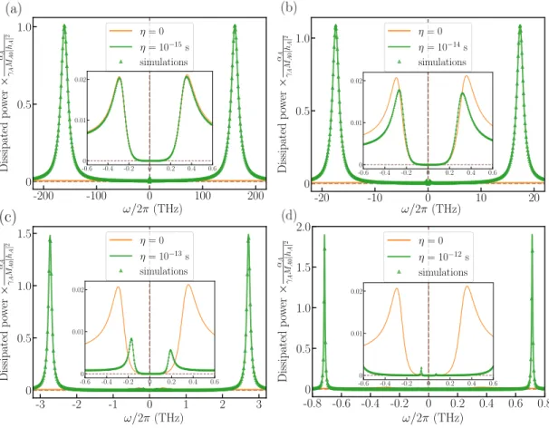
To compare with FMR, we compute the dissipated power for AFMR,P = ˙m_A·h_A+ ˙m_B·h_B, with the explicit for- mula given in AppendixC. The result is shown in Fig.2, using the same parameters for both sublattices as for the FM in Fig.1. The insets of Fig.2 show that without the inertial term the AFM precession resonance peaks are sup- pressed with respect to the FM one by a factor of about J/(2K) = 50. This is caused by the fact that the magnetization in the two sublattices rotates around the equilibrium direction with a phase shift of π, meaning that the homogeneous exciting field only couples to the difference of the sublattice precession amplitudes [14] in the dissipated power. Also, the inertial term shifts the precession resonance peaks to lower frequencies considerably stronger than in the FM, and further reduces their magnitude. At higher frequency, two additional nutation resonance peaks can be observed. Remarkably, their height is significantly larger than that of the precession resonances, even exceeding the intensity of the FMR peaks (cf. Fig. 1 where the same normalization was used). The latter suggests that probing the AFM nutation resonance peak is experimentally more

suitable than in the FM case. Most of these effects can be explained by the fact that the precession and nutation resonance frequencies lie much closer in AFMs than in FMs, as will be discussed in detail below.

To obtain the AFM resonance frequencies, we calculate the nodes of the susceptibility tensor in Eq. (4), obtaining

∆_± =a_±ω⁴+b_±ω³+c_±ω²+d_±ω+e_±= 0. (5) with the following definitions:

a_±=ηAηB, (6)

b_±=∓i(αAηB+αBηA)−(ηA−ηB), (7) c_±=−1±i(α_A−α_B)−(Ω_Aη_B+ Ω_Bη_A)

−αAαB, (8)

d_±= (ΩA−ΩB)±i(αBΩA+αAΩB), (9) e_±=− γ_A

MA0

γ_B MB0

J²+ Ω_AΩ_B. (10) Note that inertial effects enter viaa, b, andc, terms which are of higher order in frequency. Setting the inertial re-

(4)

-200 -100 0 100 200 0

0.5 1.0

Dissipatedpower£ÆA ∞AMA0|hA|2

!/2º(THz)

¥= 0

¥= 10^°¹⁵s simulations

-0.60 -0.4 -0.2 0 0.2 0.4 0.6

0.01 0.02

-20 -10 0 10 20

0 0.5 1.0

!/2º(THz)

¥= 0

¥= 10^°¹⁴s simulations

-0.6 -0.4 -0.2 0 0.2 0.4 0.6

0 0.01 0.02

-0.8 -0.6 -0.4 -0.2 0 0.2 0.4 0.6 0.8 0

0.5 1.0 1.5 2.0

!/2º(THz)

¥= 0

¥= 10^°¹²s simulations

-0.60 -0.4 -0.2 0 0.2 0.4 0.6

0.01 0.02

-3 -2 -1 0 1 2 3

0 0.5 1.0 1.5

!/2º(THz)

¥= 0

¥= 10^°¹³s simulations

-0.60 -0.4 -0.2 0 0.2 0.4 0.6

0.01 0.02

Figure 2. The rate of energy dissipation for the antiferromagnet as a function of frequency for several values of the inertial relaxation timeηA =ηB =η, (a) η = 1 fs, (b)η = 10fs, (c) η = 100fs and (d)η = 1 ps. The lines denote the results of the analytical calculations and the symbols of the atomistic spin simulations for two coupled macrospins. All curves are compared to the analytical expression obtained without the inertial term. The other parameters are MA0 = MB0 = 2µB, γA =γB = 1.76×10¹¹ T⁻¹s⁻¹, αA =αB = 0.05,KA = KB = 10⁻²³ J, J = 10⁻²¹ J, H0 = 1T, and |hA|= |hB| = 0.001 T. The insets show the precession resonances on a smaller frequency and power scale.

laxation times to zero, we obtain a second-order equation that results in well-known antiferromagnetic resonance frequencies [31–33]. For equivalent sublattices and assuming α 1 and K ≈ H0M0 J, these read ωp± ≈

1±iαp

J/(4K) γH0±γ/M√ 4KJ

. Com- pared to the FM case, two resonance frequencies are found, and they are exchange enhanced by about a factor of pJ/K. However, the lifetime of the excitations is reduced since the effective damping is also higher by a factor of pJ/(4K).

In the presence of the inertial term, the resonance frequencies are found as a solution of a fourth-order equation.

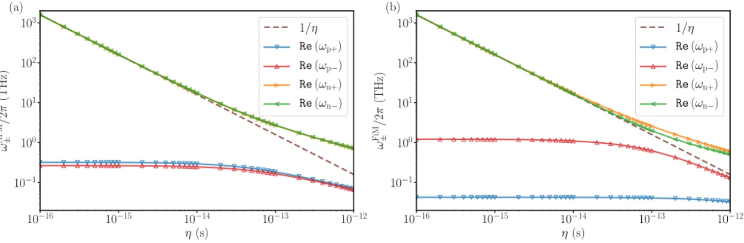
The real and imaginary parts of the calculated frequencies are denoted byRe(ω_p,n±)andIm(ω_p,n±)for precession and nutation resonances, respectively. These have been calculated for an AFM and a FiM as a function of the relaxation timeηA=ηB=ηin Fig.3. In the absence of external field and damping, Eq. (5) simplifies to a second-order equation inω². The precession resonance frequencies are given by ω_p± ≈ ±γ/M√

4KJ(1 + 2βAFM)⁻¹² for K J. It is important to note here that the relative strength of the inertial corrections is defined by the dimensionless parameter βAFM=(ηγ/M0)J, which is enhanced by a factor ofJ/Kas compared toβFM. The characteristic time scale of the ex-

change interactions typically falls into the fs range in AFMs which are ordered at room temperature (γJ/M≈10¹³s⁻¹ with the parameters used here), which is similar to the typical values of the inverse inertial relaxation time [20,23,25].

This explains the considerable decrease of the AFMR precession frequencies in Fig.2, while Fig.3(a) demonstrates that deviations from the non-inertial case already become observable for η ≈1 fs. This more pronounced inertial effect should also be observable if the resonance is measured by sweeping the external field, as in Ref. [23]. The strongly asymmetric (M_A0 = 5M_B0) FiM in Fig. 3(b) is charac- terized by a high-frequency exchange mode, strongly influenced by inertial effects as in the AFM, and a low-frequency mode which is less affected like in the FM.

The nutation resonance frequencies in the AFM can be expressed as ω_n±≈ ±√1 + 2β_AFM/η. Just as for the precession resonance, the correction factor arising due to the interplay between inertia and magnetic interactions is given byβAFM, which is exchange enhanced compared to the FM case. This gives rise to an increase of the nutation frequencies, as demonstrated in Fig. 2. For the FiM in Fig. 3(b), the nutation frequencyRe(ω_n+)belonging to the exchange mode Re(ω_p−) starts deviating from the low-inertia η⁻¹ asymptote at considerably lower frequencies than the FM- like nutationRe(ω_n−).

(5)

10⁻¹⁶ 10⁻¹⁵ 10⁻¹⁴ 10⁻¹³ 10⁻¹² η(s)

10⁻¹ 10⁰ 10¹ 10² 10³

ωAFM ±/2π(THz) (a)

1/η Re(ωp+) Re(ω_p−) Re(ωn+) Re(ω_n−)

10⁻¹⁶ 10⁻¹⁵ 10⁻¹⁴ 10⁻¹³ 10⁻¹²

η(s) 10⁻¹

10⁰ 10¹ 10² 10³

ωFiM ±/2π(THz) (b)

1/η Re(ωp+) Re(ω_p−) Re(ωn+) Re(ω_n−)

Figure 3. (Color Online) Real part of the precession resonance frequencies as a function of inertial relaxation timeη, (a) for AFMs withMA0=MB0= 2µBand (b) for FiMs withMA0= 5MB0 = 10µB. The other parameters areγA=γB = 1.76×10¹¹T⁻¹s⁻¹, αA=αB= 0.05,KA=KB= 10⁻²³J,J= 10⁻²¹J,H0= 1T.

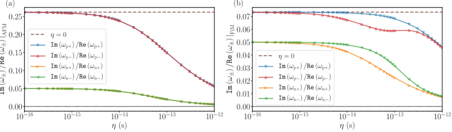
The effective damping parameters of the excitation modes, defined as the ratio of the imaginary to the real part of the frequencies, are shown in Fig.4. They no longer co- incide between precession and nutation as in the FM case, since the exchange enhancement discussed above does not affect the nutation resonance. A reduction of the effective damping is observed with increasing inertial relaxation times, which becomes noticeable forβ_AFM=O 10⁻²

, just as in the case of the resonance frequencies. The considerable reduction of the effective damping compared to the Gilbert damping leads to sharper nutation resonance peaks as demonstrated in Fig.2, with higher intensities than for the FM. In the FiM, the exchange modes ω_n+ and ω_p−

start to become influenced at lower inertial relaxation times than the FM modesωn− andωp+ [34]. The difference between the effective damping parameters vanishes between exchange and FM modes for higherη, but it remains to be observable between precession and nutation modes.

V. CONCLUSIONS

To conclude, we applied the ILLG equation to FMs and to two-sublattice AFMs and FiMs, and investigated the resonance frequencies using linear-response theory and computer simulations. The precession frequencies are found to decrease with increasing inertial relaxation time and additional high-frequency nutation peaks become observable.

Furthermore, the calculation of the resonance linewidth shows that the effect of inertia reduces the effective damping parameter. While in FMs these corrections scale with βFM =ηΩ0, in AFMs the dimensionless coupling between precession and nutation is given by βAFM = (ηγ/M0)J, which is typically several orders of magnitude higher.

Therefore, an antiferromagnetic system with higher exchange to anisotropy energy ratio and higherηwill be suitable to observe inertial effects. Such antiferromagnetic systems include NiO [35] and CrPt [36, 37], even though the characteristic inertial relaxation timeη is unknown. The FiM is observed to interpolate between the FM and AFM limits. The reduced effective damping gives rise to particularly sharp and high-intensity nutation resonance peaks in AFMs, with frequencies comparable to the values already

observed in FMs [23, 25]. These findings are expected to motivate the search for the signs of intrinsically inertial spin dynamics on ultrafast timescales using AFMR techniques.

ACKNOWLEDGMENTS

We acknowledge financial support from the Alexander von Humboldt-Stiftung, the Deutsche Forschungsgemein- schaft via Project No. NO 290/5-1, and the National Re- search, Development, and Innovation Office of Hungary via Project No. K131938.

Appendix A: Atomistic simulations of the ILLG equation

The inertial Landau-Lifshitz-Gilbert (ILLG) equation of motion, given in Eq. (1) in the main text, can be rewritten for the normalized spins_i(t) =M_i(t)/M_i0 as [21]

∂_ts_i=−γ_is_i×H_i+α_is_i×∂_ts_i+η_is_i×∂_tts_i. (A1) The first term denotes precession of the spins around an effective field Hi, the second term corresponds to a transverse relaxation of the spins, and the last term defines the inertial dynamics [15]. The ILLG equation can be rewritten from the implicit form of Eq. (A1) to an explicit differential equation which can be solved numerically without iterations. By taking a scalar product of Eq. (A1) withsiit is easy to see that the length of the spin remains conserved in the ILLG equation, i.e., ∂t|si|² = 0 and si·∂tsi = 0.

Furthermore, we use

si×(si×∂ttsi) =si(si·∂ttsi)−∂ttsi, (A2)

∂_t(s_i·∂_ts_i)

| {z }

=0

= (∂_ts_i)²+s_i·∂_tts_i. (A3)

By multiplying Eq. (A1) by s_i×and using the conditions Eqs. (A2) and (A3), we obtain the explicit equation of motion (cf. Ref. [30])

∂_tts_i=−γ_i ηi

s_i×(s_i×H_i)−α_i ηi

∂_ts_i− 1 ηi

s_i×∂_ts_i

−si(∂tsi)²=Fi(s, ∂ts, t). (A4)

(6)

10⁻¹⁶ 10⁻¹⁵ 10⁻¹⁴ 10⁻¹³ 10⁻¹² η(s)

0.00 0.05 0.10 0.15 0.20 0.25

Im(ω±)/Re(ω±)|AFM

(a)

η= 0

Im(ωp+)/Re(ωp+) Im(ω_p−)/Re(ω_p−) Im(ωn+)/Re(ωn+) Im(ωn−)/Re(ωn−)

10⁻¹⁶ 10⁻¹⁵ 10⁻¹⁴ 10⁻¹³ 10⁻¹²

η(s) 0.00

0.01 0.02 0.03 0.04 0.05 0.06 0.07

Im(ω±)/Re(ω±)|FiM

(b)

η= 0

Im(ωp+)/Re(ωp+) Im(ωp−)/Re(ωp−) Im(ωn+)/Re(ωn+) Im(ωn−)/Re(ωn−)

Figure 4. (Color Online) Effective damping parameters of the resonance modes as a function of inertial relaxation timeη, for (a) AFMs withMA0=MB0= 2µBand (b) FiMs withMA0= 5MB0= 10µB. The other parameters areγA=γB= 1.76×10¹¹T⁻¹s⁻¹, αA=αB= 0.05,KA=KB= 10⁻²³J,J= 10⁻²¹J,H0= 1T.

Note that a second-order explicit differential equation is obtained because of the inertial term, while the LLG equation is of first order. With the definitionpi=∂tsi, we can convert the second-order differential equation into a system of first-order differential equations as follows:

∂ttsi=∂tpi=Fi(s,p, t), (A5)

∂_ts_i=p_i=G_i(s,p, t). (A6) It is obvious that one has to solve six coupled differential equations of first order per lattice site i. We numerically solve these equations with Heun’s method [38], where the predictor steps are

¯

si=si(t) + ∆tGi(s,p, t), (A7)

¯

p_i=p_i(t) + ∆tF_i(s,p, t), (A8) and the corrector steps are implemented as

si(t+ ∆t) =si(t) +∆t

2 [Gi(s,p, t) +Gi(¯s,p, t¯ + ∆t)], (A9) pi(t+ ∆t) =pi(t) +∆t

2 [Fi(s,p, t) +Fi(¯s,p, t¯ + ∆t)]. (A10) In order to calculate the resonance curves, we employed a circularly polarized fieldh(t)∼e^iωt in thexyplane in ad- dition to the static magnetic fieldH0along thezdirection,

and solved the equations of motion for one and two spins by starting from the equilibrium state along the zdirection.

By multiplying Eq. (A4) byMi0ηi∂tsi/γi, summing over the sublattices, and rearranging the terms, one arrives at

∂_t X

i

M_i0η_i 2γi

(∂_ts_i)²+F

!

=X

i

∂_tM_i0∂_ts_ih_i

−X

i

αi

Mi0

γi

(∂tsi)² . (A11)

The left-hand side of Eq. (A11) describes the change of rate of the energy of the system, consisting of a kinetic part and a potential partF. The former sheds light on the meaning of ηi as an inertial parameter. The right-hand side con- sists of the power loss due to damping processes, which is compensated by the external driving force in a steady state. Accordingly, we computed the dissipated power us- ingP =P

iMi0∂tsi·hi.

Appendix B: Calculation of the linear response in ferromagnets

In ferromagnets, we consider that the initial magnetization points towards the z direction, such that the magnetization is expanded asM =M0eˆz+m(t)in linear order.

The considered dynamical field is denoted by h(t). Using the effective field in the main text, the linearized ILLG equation can be written in the following way:

∂tm=−γ







M0eˆz×H0eˆz

| {z }

= 0

+M0eˆz×2K M₀eˆz

| {z }

= 0

+M0eˆz×h(t) +m(t)×H0eˆz+m(t)×2K

M₀eˆz+m(t)×h(t)

| {z }

negligible







+ α M0







M0eˆz×∂m

∂t +m×∂m

∂t

| {z }

negligible





 + η

M0







M0eˆz×∂²m

∂t² +m×∂²m

∂t²

| {z }

negligible







. (B1)

(7)

Thus, we obtain the following two equations for the transversal components:

∂_tm_x=γM₀h_y−γH₀m_y−2γK

M₀ m_y−α∂_tm_y−η∂_ttm_y, (B2)

∂tmy =−γM0hx+γH0mx+2γK M0

mx+α∂tmx+η∂ttmx. (B3) We define Ω₀ = γ/M₀(H₀M₀+ 2K) as in the main text.

Therefore, Eqs. (B2) and (B3) can be recast as hx= 1

γM0

[Ω0mx+α∂tmx+η∂ttmx−∂tmy], (B4) h_y= 1

γM0

[Ω₀m_y+α∂_tm_y+η∂_ttm_y+∂_tm_x]. (B5) In matrix form we write

hx

hy

= 1 γM0

Ω0+α∂t+η∂tt −∂t

∂t Ω0+α∂t+η∂tt

mx

my

. (B6) We switch to the circularly polarized basis,m_±=mx±imy

andh_± =h_x±ih_y, where the equations decouple, γM0

h+

h₋

=

Ω0+α∂t+η∂tt+i∂t 0

0 Ω0+α∂t+η∂tt−i∂t

m+

m₋

. (B7) For the time dependence we considerh_±=he^±iωt, describ- ing two types of polarization with opposite handedness. We assumem±=me^±iωt. Thus, we have

he^iωt= 1 γM0

Ω₀+iαω−ηω²−ω me^iωt

⇒m+= γM0

Ω0+iαω−ηω²−ωhe^iωt, (B8) he^−iωt= 1

γM0

Ω0−iαω−ηω²−ω me^−iωt

⇒m₋= γM0

Ω₀−iαω−ηω²−ωhe^−iωt. (B9) This leads to the susceptibility given in Eq. (2). Its real and imaginary parts are derived as

Re(χ±) =γM0

Ω0−ω−ηω²

(Ω0−ω−ηω²)²+α²ω², (B10) Im(χ_±) =±γM₀ αω

(Ω₀−ω−ηω²)²+α²ω². (B11)

The dissipated power can be calculated according to its definition based on Eq. (A11),

P =∂tm·h

= (∂_tm_xh_x+∂_tm_yh_y)

=1

2(∂_tm₊h₋+∂_tm₋h₊)

=iω

2 (χ+−χ−)|h|²

=iω 2

−2iαωγM₀ (Ω0−ω−ηω²)²+α²ω²

|h|²

=ωIm(χ+)|h|². (B12)

The positions and the linewidths of the resonance peaks may be analyzed by finding the poles of the susceptibility in Eq. (B8),

ω= 1 2η

−(1−iα)± q

(1−iα)²+ 4βFM

= 1 2η

−1±a+iα 1∓a⁻¹

, (B13)

where βFM =ηΩ0 andais the single positive real solution of the fourth-order equation

a⁴− 1−α²+ 4β_FM

a²−α²= 0. (B14)

For βFM 1, one has a = 1 + 2βFM +O β_FM² . For the real parts of the frequencies, corresponding to the peak positions, one obtains ω_p ≈Ω₀(1−β_FM) and ω_n ≈

−1/η−Ω₀(1−β_FM), as described in the main text. Note that the latter expression agrees with Eq. (14) in Ref. [28], but the correction terms are different from Ref. [27], where ωn=−√1 +βFM/η ≈ −1/η−Ω0/2 1−β_FM/4

was sug- gested. It is apparent from Eq. (B13) that effective damping parameter, i.e. the ratio of the imaginary and the real parts of the frequency, is αa⁻¹ ≈ α(1−2βFM) both for the precession and the nutation peaks. The full width of the resonance peaks at half maximum can be expressed as

∆ω=ω₁−ω₂, which frequencies satisfy

Ω0−ω1−ηω₁²=−αω1, (B15)

Ω0−ω2−ηω₂²=αω2. (B16)

(8)

The ratio of the linewidth and the peak position is given by

∆ω

ω_p = (Ω0+αΩ0(1−βFM))−η(Ω0+αΩ0)²−(Ω0−αΩ0(1−βFM)) +η(Ω0−αΩ0)² Ω₀(1−β_FM)

= 2αΩ0−6αβFMΩ0

Ω₀(1−β_FM) = 2α1−3βFM

1−β_FM ≈2α(1−2βFM) (B17)

for the precession resonance, confirming that dividing the half-width at half maximum by the resonance frequency is approximately equal to the effective damping parameter described above.

Appendix C: Calculation of the linear response in two-sublattice antiferromagnets and ferrimagnets We expand the magnetization around the equilibrium direction in small deviations, MA = MA0eˆz +mA and MB = −MB0eˆz+mB, which are induced by the transverse external fieldh_A/B(t). The linearized ILLG equation for the two sublattices reads

∂tmA=− γA

MA0

[−(H0MA0+ 2KA+J)mAxeˆy+ (H0MA0+ 2KA+J)mAyeˆx] + γA

MB0

[J mBxeˆy−J mByeˆx]

−γAMA0(hAxeˆy−hAyeˆx) +αA(∂tmAxeˆy−∂tmAyeˆx) +ηA(∂ttmAxeˆy−∂ttmAyeˆx), (C1)

∂tmB=− γB

MB0

[−(H0MB0−2KB−J)mBxeˆy+ (H0MB0−2KB−J)mByeˆx]− γB

MA0

[J mAxeˆy−J mAyeˆx] +γ_BM_B0(h_Bxeˆ_y−h_Byeˆ_x)−α_B(∂_tm_Bxeˆ_y−∂_tm_Byeˆ_x)−η_B(∂_ttm_Bxeˆ_y−∂_ttm_Byeˆ_x). (C2) For thexandy components we obtain

γAMA0hAy= γA

M_A0(H0MA0+ 2KA+J)mAy+ γA

M_B0J mBy+αA∂tmAy+ηA∂ttmAy+∂tmAx, (C3) γAMA0hAx= γA

M_A0(H0MA0+ 2KA+J)mAx+ γA

M_B0J mBx+αA∂tmAx+ηA∂ttmAx−∂tmAy, (C4) γBMB0hBy= γB

M_B0(−H0MB0+ 2KB+J)mBy+ γB

M_A0J mAy+αB∂tmBy+ηB∂ttmBy−∂tmBx, (C5) γ_BM_B0h_Bx= γB

M_B0(−H₀M_B0+ 2K_B+J)m_Bx+ γB

M_A0J m_Ax+α_B∂_tm_Bx+η_B∂_ttm_Bx+∂_tm_By. (C6) In the circularly polarized basis with m_A/B± = m_A/Bx ±im_A/By, h_A/B± = h_A/Bx ±ih_A/By and defining Ω_A = γA/MA0(H0MA0+ 2KA+J),ΩB=γB/MB0(J+ 2KB−H0MB0), we obtain

γ_AM_A0h_A±= (Ω_A+α_A∂_t+η_A∂_tt±i∂_t)m_A±+ γA

M_B0J m_B±, (C7)

γ_BM_B0h_B±= (Ω_B+α_B∂_t+η_B∂_tt∓i∂_t)m_B±+ γB

M_A0J m_A±. (C8)

The four equations of motion are separated into two pairs of coupled equations for the+and −components. In matrix formalism we have

hA±

h_B±

=





 1 γAMA0

(ΩA+αA∂t+ηA∂tt±i∂t) 1 MA0MB0

J 1

MA0MB0

J 1

γBMB0

(Ω_B+α_B∂_t+η_B∂_tt∓i∂_t)





 mA±

m_B±

. (C9)

By substituting the time dependenceh_A/B±, m_A/B±∝e^±iωt we have

h_A±

h_B±

=





 1 γAMA0

ΩA±iωαA−ηAω²−ω 1 MA0MB0

J 1

MA0MB0

J 1

γBMB0





 m_A±

m_B±

. (C10)

(9)

We introduce the definition ∆_± = (γ_AM_A0γ_BM_B0)⁻¹ Ω_A±iωα_A−η_Aω²−ω

Ω_B±iωα_B−η_Bω²+ω

− J²/ M_A0² M_B0²

for the determinant of the matrix above. The susceptibility tensor is obtained by matrix inversion, m_A±

m_B±

= 1

∆_±





 1 γBMB0

− 1 MA0MB0

J

− 1 MA0MB0

J 1

γAMA0

ΩA±iωαA−ηAω²−ω





 h_A±

h_B±

=χ^AB_± h_A±

h_B±

,

(C11) as also given in Eq. (4).

Similarly to the ferromagnet, we calculate the dissipated power from Eq. (A11) as PAB=∂tmA·hA+∂tmB·hB

= 1 2 h

∂tmA+hA−+∂tmA−hA++∂tmB+hB−+∂tmB−hB+

i

= iω 2

h 1

∆+

1 γBMB0

ΩB+iωαB−ηBω²+ω

hA+− 1 MA0MB0

J hB+

hA−

− 1

∆−

1 γBMB0

Ω_B−iωα_B−η_Bω²+ω

h_A−− 1 MA0MB0

J h_B−

h_A+

+ 1

∆₊

− 1

M_A0M_B0J h_A++ 1

γ_AM_A0 Ω_A+iωα_A−η_Aω²−ω h_B+

h_B−

− 1

∆₋

− 1

M_A0M_B0J h_A−+ 1

γ_AM_A0 ΩA−iωαA−ηAω²−ω h_B−

hB+

i

= ω²|hA|² γ_BM_B0





(γ_AM_A0γ_BM_B0)⁻¹α_Ah

Ω_B−η_Bω²+ω2

+ω²α²_Bi

+J²/ M_A0² M_B0² α_B

∆₊∆₋





+ω²|hB|² γAMA0





(γ_AM_A0γ_BM_B0)⁻¹α_Bh

Ω_A−η_Aω²−ω²

+ω²α²_Ai

+J²/ M_A0² M_B0² α_A

∆+∆₋





− 2ω²J|hAhB| γ_AM_A0² γ_BM_B0²

(ΩAαB+ ΩBαA) + (αA−αB)ω−(ηAαB+ηBαA)ω²

∆₊∆₋

. (C12)

As discussed in the main text, the peak positions and the linewidths may be understood by finding the nodes of the determinant∆_±,

ΩA±iωαA−ηAω²−ω

− γ_Aγ_B MA0MB0

J²= 0

⇒ηAηB

| {z }

=a±

ω⁴+ [∓i(αAηB+αBηA)−(ηA−ηB)]

| {z }

=b±

ω³

+ [−1±i(α_A−α_B)−(Ω_Aη_B+ Ω_Bη_A)−α_Aα_B]

| {z }

=c±

ω²

+ [(Ω_A−Ω_B)±i(α_BΩ_A+α_AΩ_B)]

| {z }

=d±

ω+ Ω_AΩ_B− γ_Aγ_B MA0MB0

J²

| {z }

=e±

= 0. (C13)

The fourth-order equation (C13) may be solved in a closed form. However, in order to arrive at solutions which have a simpler form, we consider the antiferromagnet with identical sublattices, M_A0 = M_B0 =M₀, α_A = α_B = α, ηA = ηB = η, and KA = KB = K. Furthermore, we assume α 1 and M0H0, K J, as is typical in most systems. Consequently, we will treat the terms propor- tional to the damping and the external field in first-order

perturbation theory, leading to η²ω⁴−

1 + 2η γ

M₀(J+ 2K)

ω²−i2αηω₍₀₎³ + 2γH0ω₍₀₎ +i2α γ

M0

(J+ 2K)ω₍₀₎+ γ²

M₀²(J+ 2K)²−γ²(H₀)²

− γ²

M₀²J²= 0, (C14)

where ω₍₀₎ is the solution for α= 0and H0 = 0, and we

(10)

only treat ∆₊ for simplicity since ∆₋ may be obtained by complex conjugation. Equation (C14) is a second-order equation inω², the solutions of which are simple to express.

Expanding them up to first order in αand H₀ for consis- tency with the order of the perturbation, and also in first order inK/J1, one obtains

ω_p±≈ ± γ M0

p4K(J +K) r

1 + 2η γ M0

(J+ 2K)

+ 1

r

1 + 2η γ M0

(J+ 2K)

×

ω₍₀₎ γ

M0

p4K(J+K)

γH0+iα γ

M₀(J+ 2K)−ηω₍₀₎²

, (C15)

ω_n±≈ ±1 η

r

1 + 2η γ M0

(J+ 2K)





 1−

η² γ²

M₀²4K(J+K) 2

1 + 2η γ M0

(J+ 2K) 2







− η

ω₍₀₎

1 + 2η γ M0

(J+ 2K) ³₂

γH₀+iα γ

M0

(J+ 2K)−ηω²₍₀₎

, (C16)

for the precession and the nutation frequencies, respectively. Substituting in ω₍₀₎

from the leading term in the expression into the perturbative terms, one arrives at

ω_p±≈ ± γ M0

p4K(J+K) r

1 + 2η γ M0

(J+ 2K)

+ 1

1 + 2η γ

M₀(J+ 2K)

γH₀+iα γ

M₀(J+ 2K)

, (C17)

ωn±≈ ±1 η

r

1 + 2η γ M0

(J+ 2K)





 1−

η² γ²

M₀²4K(J+K) 2

1 + 2η γ M0

(J+ 2K) 2







− 1

1 + 2η γ M0

(J+ 2K)

γH0−iα 1

η + γ M0

(J+ 2K)

. (C18)

The leading-order terms forH0, α= 0and usingJ+K≈ J are also reported in the main text. As discussed there, in the antiferromagnet the corrections caused by the inertial dynamics surpass in magnitude those in the ferromagnet, since the characteristic dimensionless parameter βFM = ηΩ0 is replaced by βAFM = ηγ/M0(J+ 2K) ≈ ηγ/M0J+2K. This difference is also manifest in the dependence of the excitation frequencies on the static magnetic field H₀: while in the ferromagnet the Larmor frequency is renormalized as (1−β_FM)γH₀, in the antiferromagnet the corresponding factor is(1 + 2βAFM)⁻¹γH0for both the precession and the nutation frequencies, causing an apparent decrease in the gyromagnetic factor.

From Eqs. (C17) and (C18), the effective damping pa-

rameters in the antiferromagnet may be expressed as Im(ω_p)

Re(ωp) ≈α s

(J+ 2K)² 4K(J+K)

1 r

1 + 2η γ

M₀(J+ 2K) ,

(C19) Im(ω_n)

Re(ωn) ≈α

1 +η γ

M₀(J+ 2K)

1 + 2η γ M0

(J+ 2K) ³₂

. (C20)

While the inertial dynamics decrease the resonance linewidth of the antiferromagnet by a larger factor (1 + 2β_AFM)^−1/2compared to the ferromagnet(1−2β_FM), this is compensated by the exchange enhancement expressed in the factor p

J/4K. Remarkably, the effective damping of the nutation resonance is not exchange en-

(11)

hanced, while it is still reduced compared to the Gilbert damping due to the inertial motion, giving rise to the particularly sharp peaks in Fig.2.

[1] C. D. Stanciu, F. Hansteen, A. V. Kimel, A. Kirilyuk, A. Tsukamoto, A. Itoh, and T. Rasing, Phys. Rev. Lett.

99, 047601 (2007).

[2] K. Vahaplar, A. M. Kalashnikova, A. V. Kimel, D. Hinzke, U. Nowak, R. Chantrell, A. Tsukamoto, A. Itoh, A. Kiri- lyuk, and T. Rasing,Phys. Rev. Lett.103, 117201 (2009).

[3] I. Radu, K. Vahaplar, C. Stamm, T. Kachel, N. Pontius, H. A. Dürr, T. A. Ostler, J. Barker, R. F. L. Evans, R. W.

Chantrell, A. Tsukamoto, A. Itoh, A. Kirilyuk, T. Rasing, and A. V. Kimel,Nature472, 205 (2011).

[4] K. Vahaplar, A. M. Kalashnikova, A. V. Kimel, S. Ger- lach, D. Hinzke, U. Nowak, R. Chantrell, A. Tsukamoto, A. Itoh, A. Kirilyuk, and Th. Rasing, Phys. Rev. B 85, 104402 (2012).

[5] A. Hassdenteufel, B. Hebler, C. Schubert, A. Liebig, M. Te- ich, M. Helm, M. Aeschlimann, M. Albrecht, and R. Brats- chitsch,Advanced Materials25, 3122 (2013).

[6] A. V. Kimel, B. A. Ivanov, R. V. Pisarev, P. A. Usachev, A. Kirilyuk, and Th. Rasing,Nat. Phys.5, 727 (2009).

[7] S. Wienholdt, D. Hinzke, and U. Nowak,Phys. Rev. Lett.

108, 247207 (2012).

[8] L. D. Landau and E. M. Lifshitz, Phys. Z. Sowjetunion8, 101 (1935).

[9] T. L. Gilbert and J. M. Kelly, in

American Institute of Electrical Engineers (New York, October 1955) pp. 253–263.

[10] T. L. Gilbert, IEEE Transactions on Magnetics 40, 3443 (2004).

[11] L. Rózsa, S. Selzer, T. Birk, U. Atxitia, and U. Nowak, Phys. Rev. B100, 064422 (2019).

[12] E. V. Gomona˘i and V. M. Loktev,Low Temp. Phys. 34, 198 (2008).

[13] K. M. D. Hals, Y. Tserkovnyak, and A. Brataas,Phys. Rev.

Lett.106, 107206 (2011).

[14] A. G. Gurevich and G. A. Melkov,

Magnetization Oscillations and Waves, Lecture Notes in Physics (CRC Press, 1996).

[15] M.-C. Ciornei, J. M. Rubí, and J.-E. Wegrowe,Phys. Rev.

B83, 020410 (2011).

[16] J.-E. Wegrowe and M.-C. Ciornei, Am. J. Phys. 80, 607 (2012).

[17] D. Böttcher and J. Henk,Phys. Rev. B86, 020404 (2012).

[18] M. Fähnle, D. Steiauf, and C. Illg,Phys. Rev. B84, 172403 (2011).

[19] M. Fähnle and C. Illg, J. Phys.: Condens. Matter 23,

493201 (2011).

[20] S. Bhattacharjee, L. Nordström, and J. Fransson, Phys.

Rev. Lett.108, 057204 (2012).

[21] R. Mondal, M. Berritta, A. K. Nandy, and P. M. Oppeneer, Phys. Rev. B96, 024425 (2017).

[22] R. Mondal, M. Berritta, and P. M. Oppeneer, J. Phys.:

Condens. Matter30, 265801 (2018).

[23] Y. Li, A.-L. Barra, S. Auffret, U. Ebels, and W. E. Bailey, Phys. Rev. B92, 140413 (2015).

[24] D. Thonig, O. Eriksson, and M. Pereiro, Sci. Rep.7, 931 (2017).

[25] K. Neeraj, N. Awari, S. Kovalev, D. Polley, N. Zhou Hagström, S. S. P. K. Arekapudi, A. Semisalova, K. Lenz, B. Green, J.-C. Deinert, I. Ilyakov, M. Chen, M. Bawatna, V. Scalera, M. d’Aquino, C. Serpico, O. Hell- wig, J.-E. Wegrowe, M. Gensch, and S. Bonetti,Nat. Phys.

(2020),https://doi.org/10.1038/s41567-020-01040-y.

[26] E. Olive, Y. Lansac, and J.-E. Wegrowe,Appl. Phys. Lett.

100, 192407 (2012).

[27] E. Olive, Y. Lansac, M. Meyer, M. Hayoun, and J.-E. We- growe,J. Appl. Phys.117, 213904 (2015).

[28] M. Cherkasskii, M. Farle, and A. Semisalova, Nutation resonance in ferromagnets (2020),arXiv:2008.12221 [cond- mat.mes-hall].

[29] I. Makhfudz, E. Olive, and S. Nicolis, Appl. Phys. Lett.

117, 132403 (2020).

[30] T. Kikuchi and G. Tatara,Phys. Rev. B92, 184410 (2015).

[31] C. Kittel,Phys. Rev.82, 565 (1951).

[32] F. Keffer and C. Kittel,Phys. Rev.85, 329 (1952).

[33] A. Kamra, R. E. Troncoso, W. Belzig, and A. Brataas, Phys. Rev. B98, 184402 (2018).

[34] F. Schlickeiser, U. Atxitia, S. Wienholdt, D. Hinzke, O. Chubykalo-Fesenko, and U. Nowak, Phys. Rev. B86, 214416 (2012).

[35] M. T. Hutchings and E. J. Samuelsen,Phys. Rev. B6, 3447 (1972).

[36] M. J. Besnus and A. J. P. Meyer, phys. stat. sol. (b)58, 533 (1973).

[37] R. Zhang, R. Skomski, X. Li, Z. Li, P. Manchanda, A. Kashyap, R. D. Kirby, S.-H. Liou, and D. J. Sellmyer, J. Appl. Phys.111, 07D720 (2012).

[38] U. Nowak, Handbook of Magnetism and Advanced Mag- netic Materials (2007).