Online Calibration of Microscopic Road Trafﬁc Simulator

(1)

Online Calibration of Microscopic Road Traffic Simulator

1^st Xuan Fang

Dept. of Control for Transportation and Vehicle Systems Fac. of Transportation Eng. and Vehicle Eng.

Budapest University of Technology and Economics Budapest, Hungary

fang.xuan@mail.bme.hu

2^nd Tam´as Tettamanti

tettamanti@mail.bme.hu

3^rd Arthur Couto Piazzi

piazzi.arthur@mail.bme.hu

Abstract—Microscopic road traffic simulator is a powerful tool to analyze and evaluate various transportation systems due to its efficiency and risk-free operation. It is, therefore, widely used in traffic engineering field along with the gradual implementation of novel intelligent transportation systems. A reliable microscopic traffic simulator is able to accurately represent the real-world traffic situation when it is effectively calibrated with the combination of field data and proper simulation settings. Based on the existing theoretical calibration framework for the microscopic traffic simulator, this paper proposes an online calibration procedure using genetic algorithm as well as a specific implementation method to provide real-time performance measures that adequately mimic the field traffic situation. The proposed method was tested based on loop detector data demonstrating that real-time traffic modeling can be run in parallel with the real-world traffic process.

Index Terms—real-time traffic modeling, microscopic traffic simulation, calibration, genetic algorithm

I. INTRODUCTION

In recent years, rapid growth of urban mobility demand is getting urban traffic network much more crowded [1]. As a result, effective traffic management is becoming one of the most pressing problems in big metropolitan areas. Urban road traffic network is a complex system with randomness and uncertainty, it is difficult to formulate a corresponding solution for a specific traffic situation in advance due to its complex.

In addition, due to the randomness and the destructiveness of assessing the safety of transportation systems, it is not possible to conduct research by direct experimentation. There- fore, applying simulation technology in the field of traffic management and theoretical transport research has become a handful method. At present, traffic simulation is an integral part of intelligent transportation systems (ITS) to improve traffic management efficiency. Moreover, the advent of auto- mated vehicles also indicates that an intensive use of traffic simulation shall contribute to a better traffic management for future transportation [2], [3].

Traffic simulation refers to the interaction of models de- scribing the characteristics and behavior of each vehicle unit in the transportation system via computer technology. Due to microscopic traffic simulation has benefits on the low simulation cost, simulation without any risk, and fast simulation run time, it has been intensively applied for designing and operation of traffic management systems [4]. To provide a credible microscopic traffic simulation, calibration must be performed to guarantee that the established model truly reflects the real world traffic situation. This process is generally implemented by comparing the field measurements to the corresponding simulation output [5]. Numerous studies have yielded results in terms of providing credible methods such as trial-and-error methods, genetic algorithm (GA), simultaneous perturbation stochastic approximation (SPSA) [6]–[9]. Another part of the research focuses on the calibration process, a representative one is the 7-step calibration framework proposed by Hellinga in 1998 [10] which many subsequent studies [11]–[13] were based on. Unlike the research mentioned above using historical static data during the calibration process, this paper solely applies the previous simulation step output as initial data of the next step to achieve the online calibration of the microscopic road traffic simulator, i.e. in this way real-time traffic modeling can be realized based on online traffic sensor measurements.

The paper is organized into four chapters: this introduction, a description of the calibration algorithm and the implemented framework, a description of how the proposed calibration process was tested on an urban intersection, as well as a conclusion.

II. MICROSCOPICROADTRAFFICSIMULATOR ONLINE

CALIBRATION AND IMPLEMENTATION

A. Design of The Calibration Algorithm

Microscopic traffic simulator calibration is performed by selecting one or more parameters and then repeatedly com-

(2)

paring the measured data with the simulation output until the preset error range is reached. This process can be seen as a complex optimization problem with huge search space.

There is no specific functional relationship between the fitness function and the parameter to be calibrated in such kind of optimization problem, therefore, computing based artificial intelligence methods such as simulated annealing, GA, SPSA were applied. The most widely used among all these was GA.

The main advantage of GA is that it is able to search solutions under multiple criteria, which increases the probability of finding a global solution rather than a local optimal solution [14].

Before using GA, the parameters to be calibrated need to be coded to obtain the individual used in the algorithm, and the problem to be solved is transformed into the fitness function.

Then GA will find the individual with the smallest value of the fitness function, and then decode, get the solution to the original problem. When calculating GA, starting from a randomly generated population which is a group of individuals that corresponding to a feasible solution to the original optimization, GA will compare the fitness value of each individual in each generation, and select individuals with the smallest fitness value, and with the help of genetic operators, individuals are selected to crossover and mutate to produce new populations. According to the survival of the fittest law, individuals who are more adapted to the environment will be evolved, that is, the fitness value is more approach to the required solution. In past researches, various fitness functions were used to minimize the discrepancies between field measurement and simulation output, representative of these were root mean square percent error [15], root mean square error (RMSE), mean absolute error (MAE), global relative error (GRE) [16], and GEH statistic [17]. In this paper, the L_∞−norm of relative error is used to form the fitness function in the calibration process. The calibration problem using average traffic volume as performance measures can be written as follows:

min_Q(k)

n

X

i=1

w w w w

F¯_i^{M easured}(k)−F¯_i^Simulated Q(k) F¯_i^{M easured}(k)

w w w w∞

Where:

• F¯_i^{M easured}(k) is the average traffic volume of edge i from the ground truth at stepk;

• F¯_i^Simulated Q(k)

represents the average traffic volume of edge i produced by the calibrated simulator in the previous simulation time windowk;

• Q(k)represents the applied calibration parameter.

During the microscopic simulation, driver behavior, traffic flow characteristics are described by numerous independent microscopic parameters, and the different setting of these parameters affect the simulation output a lot. Using the default model parameter settings will cause the simulated output such as the vehicle number, lane occupancy, traffic density have large errors compared with the measured values in the field. In

order to eliminate the influence of these errors on the calibration process, simulated measurements based on real traffic data are used as the ground truth which represents the field measures. In this paper, Edge-Based measurements which simulate induction loop detector measures are used as ground truth.

The simulation output for the same edge can be aggregated to generate the performance measures, that is ”Average traffic volume (veh/h) = speed(m/s)∗3.6∗density(veh/km)”.

B. Online Calibration Process

The microscopic traffic simulator online calibration based on GA follows the subsequent steps:

• Define the research objectives and the overall framework;

• Data collection and preprocessing;

• Create microscopic simulation model;

• Model error review and correction;

• Online calibration using GA;

• Results analysis;

• Final report and technical documentation.

In the first step, an overall framework based on the research objectives is clarified including define the specific problem that need to be solved, establish suitable data archiving mechanism.

Microscopic traffic simulation usually requires several in- puts: road static geometric data (road length, the number of lanes, etc.); traffic control data (signal control schema, give way rules, prohibiting left turn, etc.); dynamic model demand data (flow, turning rate, etc.); calibration data (capacity, travel time, average speed, etc.).

Microscopic traffic simulation modeling is usually divided into several parts, first establishing a static road network and then setting traffic control rules. On this basis, fuse the traffic demand and other network operation data. After the model was established, error checking and the correction needs to be implemented to make sure that the established model truly reflects the field traffic situation.

The main steps of the model calibration include selecting a few finite key parameters and importing them into the model for a large number of simulations. By comparing the simulated data with the measured data, the optimal values of the selected parameter are finally filtered out.

During the results analysis, model calibration work is obtained through a large number of iterations.The representative parameter values are summarized and analyzed, so that the feedback of model calibration work on the practicality of model parameters itself can be completed, which has positive practical significance.

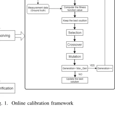
The final report and technical documentation records the results of simulation analysis in the form of reports and documents that can be presented to others. Fig. 1 shows the whole calibration framework.

The whole calibration process was implemented through the Distributed Evolutionary Algorithms in Python (DEAP), which is a computation framework for rapid testing of new ideas. Unlike other GA supporting tools such as provided by Matlab software, DEAP provides the essential bonding for assembling complex Evolutionary Computation (EC) systems

(3)

Fig. 1. Online calibration framework

rather than give a prepared or sealed solution. The goal of DEAP is to provide a practical tool for rapid custom prototyping algorithms, where each step of the process is as clear as possible and easy to read and understand [18]. The first thing to do when using the DEAP framework is defining the appropriate type for the problem. In this paper, a ”FitnessMin”

class which minimizes the problem and an individual class that is derived from a list with a fitness attribute was created.

DEAP provides an easy mechanism to fill the created types with some random value. This research creates the initializes for individuals containing random integer numbers from 1 to 200 and for a population that contains individuals.

The core of GA is three operators, namely mutation, crossover and selection, each with its own characteristics, which can be used to generate new individuals in different ways. The general rule of the mutation operator is that it involves only one individual, where a part of its genes will remain unchanged whether the rest genes accept the change (mutation). Two kinds of mutation were proposed in this research (Gaussian mutation and Uniform mutation). The Gaussian mutation generates a random number obeying the normal distribution with a meanµand a varianceσto replace the real number in the original gene. The Uniform mutation replaces the original gene value in the individual with a random probability that matches a uniformly distributed random number within a certain range. The rate of mutation determines the magnitude of the individual change that will result in the mutated individual that constitutes the next generation of individuals. To avoid random search, the small mutation rate was suggested, while the mutation rate that is too small may hardly change individuals, leading to very slow convergence.

The general rule of crossover operators is that they will com-

bine the genes of two or more individuals. The crossover operation can be performed in several ways (two-point crossover, binary crossover, uniform crossover), here executes a blend crossover. This operation is a linear combination of two parents xi andyi. The operation is initialized by choosing a uniform random real number from the interval[min(xi, yi)− α

(yi−xi)

, max(xi, yi)+α

(yi−xi)

], whereαis the positive real parameter,α= 0.1 is selected in this research.

In the evolution process, individuals that are more adaptable to the environment will have more opportunities to inherit to the next generation, the selection operator used to imitate this process. There are several selection strategies: Roulette Wheel selection, Stochastic Universal Sampling, Tournament selection and Boltzmann selection. Due to the high efficiency and easy implementation of the tournament selection algorithm, it is the most popular selection strategy in genetic algorithms.

The strategy is also very intuitive, extract n individuals from the entire population and let them compete, then extract the best individuals among them. Since the first selection is made without considering the fitness values, weak individuals can survive until the next generation, which is good for genetic variability, high values of tournament size can compromise variability, where low value can approximate to the random selection. The number of individuals participating in the tournament becomes the tournament size. Table I shows the genetic operators set in this paper.

TABLE I THE GENETIC OPERATORS

genetic operators method parameter mutation Gaussian mutation µ=0,σ=5

Uniform mutation lower bound=1, upper bound= 200 crossover blend crossover α= 0.1 selection tournament selection tournament size=3

With all above registered functions, GA was operated using the following settings:

• The probability with which two individuals are crossed is 0.5;

• The probability for mutating an individual for both Gaus- sian mutation and Uniform mutation are 0.1;

• The simulation period is 1 hour and the step interval is 5 minutes;

• The number of generations is 50;

• Two stop criteria were adopted for GA, the norm of relative error ≤0.2 or reaches 50 generations.

III. CASE STUDY

To evaluate the proposed calibration algorithm, a network based on an open database named OpenITS Research Pro- gram was generated in the Simulation of Urban MObility (SUMO), which was developed by the German Aerospace Center (DLR) in 2001. SUMO is a microscopic, multi-model traffic simulation open source technology package used to simulate the movement trajectory of vehicles operating on the network. Related traffic data was obtained considering a one

(4)

hour interval of the morning peak, from 7:00 to 8:00 on March 26, 2015. The field traffic flow data were aggregated into 300 seconds count.

A. Simulation establishment

The reliability of microscopic simulation is based on the accuracy of input data, so the investigation of field traffic data should be detailed. These data are usually the data needed to establish the road network simulation model, including the road geometry data, traffic demand data and traffic control data. This paper takes the open data of an intersection of Ningxi Road and Xingye Road, the main road in the Xi- angzhou District of Zhuhai City, China as an example, Fig.2 shows the road geometry data and satellite map of the intersection. This open database is collected by the OpenITS research program which aims to unite intelligent transportation related research institutions, teams and individuals with the concept of “openness, synergy and innovation” to jointly promote the development of intelligent transportation system research and technology application with big data as the core and support a variety of participants, including scientists, engineers, industry and students in the transportation sector.

Fig. 2. The road geometry and satellite map of the intersection

The road network not only reflects the topology of the road network itself, but also reproduces the geometric characteristics of the road, the condition of the traffic lane, the layout of signal lights, and the surrounding environment. The road network data of the intersection of Ningxi Road and Xingye Road is from Open Street Map (OSM), an open source map data providing website. Due to its open source property, the OSM map data can be different from the real world one.

After convert the OSM map data into the eXtensible Markup Language (XML) format using the ”Netconvert” program in SUMO, the network can be modified visually in the ”Netedit”

program according to the actual road topology data. The resulting road network includes 11 nodes and 11 edges. Also, the traffic light control scheme (green time, offset, duration) can be edited visually in the ”Netedit” program. This operation will generate a ”tlLogic” elements in the network file where users can also edit the traffic light scheme.

After the road network is generated, it can be viewed on the SUMO-GUI, but there is no vehicle running on the network.

The next step is to model the traffic demand. Regarding the description of traffic demand, ”trip” describes a car from the starting edge to the destination edge and the time of

departure, ”route” is a generalized trip which means that route does not only contain the starting edge and the ending edge, it also including all edges that vehicles have passed during the trip. SUMO uses ”route” to define the path of the vehicle traveling on the network. The comprehensiveness and richness of traffic information correspond to different traffic demand generation methods. According to the available traffic data provides by the OpenITS database, this paper uses flow definition to generate demand through a Python module named ”xml.etree.ElementTree” which achieves a rapid and efficient Application Programming Interface (API) for parsing and compiling XML format documents. To create route files using “xml.etree.ElementTree”, two XML files and a comma- separated values (CSV) format file that contains field traffic flow data are need, one XML file gives the template route file shows how is the flow in different direction, the CSV file gives the specific vehicle number distribution and another XML file stores the final route file.

With the net file and route file, simulation can be operated through command line application and a graphical application named ”SUMO-GUI” which can render the performed simulation visually.

B. Calibration result verification and analysis

Since GA is a random search method, the speed and result of each search may be different, the calculation time for each interval takes an average of about 1 hour. In multiple simulation steps, it is possible to converge the vicinity of the above solution within 30 generations. There is no obvious change in the operation until 50 generations. The fluctuation of the fitness function value can be observed in Fig.3.

Fig. 3. The fluctuation of fitness function value

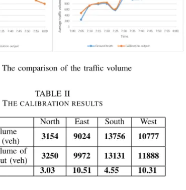
The average traffic volume, (i.e. flow) of the simulation time interval on each edge in the network is measured.

Fig. 4 depicts the traffic flow from four directions. Edge based measurements of the simulation output based on the real traffic counts is taken as the default value (represented by ”Ground truth”), and the result of simulation calibrated output (represented by ”Calibration output”) are compared.

The mean absolute percentage error (MAPE) was used as validation criteria for the proposed calibration framework, the results shown in Table II.

(5)

Fig. 4. The comparison of the traffic volume

TABLE II THE CALIBRATION RESULTS

North East South West Total Traffic volume

of ground truth (veh) 3154 9024 13756 10777 Total Traffic volume of

calibration output (veh) 3250 9972 13131 11888

MAPE (%) 3.03 10.51 4.55 10.31

The smallest difference of total traffic volume between ground truth and calibrated output occurred in the North direction of the intersection which was 3.03% and the mean absolute percentage error in each direction of the intersection was less than 11%. As Fig. 4 shows, the discrepancy in the East direction was a bit bigger than other directions, which probably caused by the non controlled edge on the network. When checking the simulation visually in SUMO- GUI, vehicles operating on the edges belonging to the East direction show more stochastic behavior due to the existence of the right turn lane (which is not controlled by traffic signal).

IV. CONCLUSION

In this paper, a framework based on intelligent heuristics optimization method (i.e. Genetic Algorithm) was developed for online calibration of real-time microscopic traffic modeling under the SUMO-DEAP environment. The whole calibration process was implemented in a case study which takes an intersection from an open database as the scenario. Based on the real traffic counts, a route file was created and imported to the SUMO simulator and edge based measurements of the simulation output were considered as ground truth. The virtually measured average traffic volume was used within the fitness function to minimize the difference between the ground truth and the calibration output. According to the validation results, all the calibrated simulation output can fit to the ground truth in a certain degree (the mean absolute percentage errors remained under 11%) which demonstrates that GA can be seen as a satisfied method to calibrate the microscopic traffic simulator.

The running time of calibration for each interval in this study is quite long due to the python script did not successfully

communicate with SUMO using the Traffic Control Interface (TraCI), which can make the algorithm obtain real-time traffic information from SUMO as well as control and edit the traffic status outside the simulation. The future work will be done to significantly reduce the executing time.

V. ACKNOWLEDGMENT

The paper was supported by the J´anos Bolyai Research Scholarship of the Hungarian Academy of Sciences as well as by the ´UNKP-19-4 New National Excellence Program of the Ministry for Innovation and Technology.

REFERENCES

[1] L. Kisgy¨orgy and A. Szele, “Traffic operation on a road Network with recurrent congestion,” Transactions on The Built Environment, vol. 179, pp. 233-243., 2018. https://doi.org/10.2495/UG180221

[2] Cs. Csisz´ar, D. F¨oldes and Y. He, “Reshaped Urban Mobility,”

Urban Design LONDON: IntechOpen Limited, pp. 1-17, 2019.

http://doi.org/10.5772/intechopen.89211

[3] T. Derenda, M. Zanne, M. Zöldy and A. Török, “Automatization in road transport: a review,” Production Engineering Archive, vol. 20, pp. 3-7, 2018.

[4] B. Ciuffo, V. Punzo, and V. Torrieri, “Comparison of Simulation- Based and Model-Based Calibrations of Traffic-Flow Microsimulation Models,” Transportation Research Record: Journal of the Transportation Research Board, vol. 2088, no. 1, pp. 36–44, 2008.

[5] D. K. Hale, C. Antoniou, M. Brackstone, D. Michalaka, A. T. Moreno, and K. Parikh, “Optimization-based assisted calibration of traffic simulation models,” Transportation Research Part C: Emerging Technologies, vol. 55, pp. 100–115, 2015.

[6] L. Chu, H. Liu, J.-S. Oh, and W. Recker, “A calibration procedure for microscopic traffic simulation,” Proceedings of the 2003 IEEE International Conference on Intelligent Transportation Systems.

[7] R.-L. Cheu, X. Jin, K.-C. Ng, Y.-L. Ng, and D. Srinivasan, “Calibration of FRESIM for Singapore Expressway Using Genetic Algorithm,”

Journal of Transportation Engineering, vol. 124, no. 6, pp. 526–535, 1998.

[8] T. Tettamanti, Z. ´A. Milacski, A. L˝orincz, and I. Varga, “Iterative Calibration Method for Microscopic Road Traffic Simulators,” Periodica Polytechnica Transportation Engineering, 2014.

[9] J. Ma, H. Dong, and H. M. Zhang, “Calibration of Microsimulation with Heuristic Optimization Methods,” Transportation Research Record:

Journal of the Transportation Research Board, vol. 1999, no. 1, pp.

208–217, 2007.

[10] Hellinga, Bruce R. “Requirements for the calibration of traffic simulation models,” Proceedings of the Canadian Society for Civil Engineering, vol.4, pp. 211-222, 1998.

[11] B. (B. Park and J. D. Schneeberger, “Microscopic Simulation Model Calibration and Validation: Case Study of VISSIM Simulation Model for a Coordinated Actuated Signal System,” Transportation Research Record: Journal of the Transportation Research Board, vol. 1856, no. 1, pp. 185–192, 2003.

[12] T. Toledo, M. E. Ben-Akiva, D. Darda, M. Jha, and H. N. Koutsopoulos,

“Calibration of Microscopic Traffic Simulation Models with Aggregate Data,” Transportation Research Record: Journal of the Transportation Research Board, vol. 1876, no. 1, pp. 10–19, 2004.

[13] J. Hourdakis, P. G. Michalopoulos, and J. Kottommannil, “Practical Procedure for Calibrating Microscopic Traffic Simulation Models,”

Transportation Research Record: Journal of the Transportation Research Board, vol. 1852, no. 1, pp. 130–139, 2003.

[14] K.-O. Kim and L. Rilett, “Genetic-algorithm based approach for calibrating microscopic simulation models,” ITSC 2001. 2001 IEEE Intelligent Transportation Systems. Proceedings (Cat. No.01TH8585).

[15] R. Balakrishna, C. Antoniou, M. Ben-Akiva, H.N. Koutsopoulos, and Y. Wen, “Calibration of microscopic traffic simulation models: Methods and application,” Transportation Research Record, vol. 1999, no. 1, pp.

198–207, 2007.

[16] T. Ma and B. Abdulhai, “Genetic Algorithm-Based Optimization Ap- proach and Generic Tool for Calibrating Traffic Microscopic Simulation Parameters,” Transportation Research Record: Journal of the Transporta- tion Research Board, vol. 1800, no. 1, pp. 6–15, 2002.

(6)

[17] A. Paz, V. Molano, E. Martinez, C. Gaviria, and C. Arteaga, “Calibration of traffic flow models using a memetic algorithm,” Transportation Research Part C: Emerging Technologies, vol. 55, pp. 432–443, 2015.

[18] F.-M. D. Rainville, F.-A. Fortin, M.-A. Gardner, M. Parizeau, and C.

Gagn´e, “Deap,” Proceedings of the fourteenth international conference on Genetic and evolutionary computation conference companion - GECCO Companion 12, 2012.