Mária Földvári
Handbook of
thermogravimetric system of minerals and its use in geological practice
Budapest, 2011
Handbook of
thermogravimetric system of minerals and
its use in geological practice
Mária Földvári
BUDAPEST, 2011
Occasional Papers of the Geological Institute of Hungary,
volume 213
© Copyright Geological Institute of Hungary (Magyar Állami Földtani Intézet), 2011 All rights reserved! Minden jog fenntartva!
Serial editor — Sorozatszerkesztő GYULAMAROS
Reviewer — Lektor:
GYÖRGYLIPTAY
English text — Angol szöveg:
MÁRIAFÖLDVÁRI
Linguistic revewer — Nyelvi lektor:
MCINTOSHWILLIAMRICHÁRD
Technical editor — Műszaki szerkesztő OLGAPIROS, DEZSŐSIMONYI
DTP
DEZSŐSIMONYI, OLGAPIROS, Cover design — Borítóterv
DEZSŐSIMONYI
Printing house — Nyomda:
Innova-Print Kft.
Published by the Geological Institute of Hungary — Kiadja a Magyar Állami Földtani Intézet
Responsible editor — Felelős kiadó TAMÁSFANCSIK
director — igazgató
This book has been subsidized by the Committee on Publishing Scientific Books and Periodicals of Hungarian Academy of Sciences
A könyv a Magyar Tudományos Akadémia Könyv- és Folyóiratkiadó Bizottságának támogatásával készült
ISBN 978-963-671-288-4
Index of Figures . . . . Index of Tables . . . . Preface . . . . Measurement methods and system of thermal reaction of minerals . . . . Introduction to the thermoanalytical methods . . . . Thermoanalytical techniques . . . . Differential Thermal Analysis (DTA) . . . . Thermogravimetry (TG) . . . . Evolved Gas Analysis (EGA) . . . . Derivative technique . . . . Multiple techniques . . . . Experimental conditions . . . . Thermoanalytical parameters . . . . Nomenclature of DTA and TG curves . . . . Description of the shape of thermoanalytical curves (DTA, DTG) . . . . Calibration . . . . Temperature and DTA calibration . . . . Evaluation of DTA peak resolution . . . . Other materials usually used for calibration . . . . Heat of reaction (∆H) . . . . TG calibration . . . . DTG calibration . . . . Effects influencing thermoanalytical curves . . . . Standardization . . . . Recommendations of ICTA Nomenclature Committee for reporting Thermal Analysis results . . . . Thermogravimetric investigation techniques and methods . . . . Techniques . . . . Quantitative determination based on mass-change . . . . Derivative Thermogravimetry (DTG, DDTG) . . . . Sample controlled Thermal Analysis (or controlled rate Thermal Analysis) . . . . Coupled simultaneous techniques, EGA methods . . . . Methods . . . . Calculation of virtual kinetic parameters . . . . Corrected decomposition temperature . . . . Supplementary methods . . . . Characteristic thermal reactions of mineral groups . . . . Thermal activity of minerals . . . . System of thermal decomposition reactions . . . . Water in minerals. Dehydration . . . . Adsorbed water . . . . Interlayer waters bond by phyllosilicates . . . .
“Zeolitic water” . . . . Water in amorphous phases . . . . Water found in completely confined internal spaces . . . . Water bound in solid solution . . . . Crystal hydrates (constitutional water in water-bearing carbonate, sulphate, phosphate and salt minerals) Thermal dissociation . . . . Other thermal reactions with mass change (sublimation, oxidation, reduction) . . . .
7 11 13 15 16 16 16 17 17 17 17 17 17 18 19 19 19 20 20 20 20 20 20 21 21 22 22 22 23 23 24 25 25 26 27 27 27 28 28 29 29 36 36 37 38 38 40 43
CONTENTS
4
Other thermal reactions without mass change . . . . Solid-phase structural decomposition . . . . Polymorphic transition . . . . Melting . . . . Curie point . . . . Solid phase reaction . . . . Thermogravimetric curves and their interpretation by stoichiometric processes of minerals . . . . 1. Native elements . . . . 1.1. Sulphur: S . . . . 1.2. Graphite C . . . . 1.2.1. Analysis in air . . . . 1.2.2. Analysis in oxygen . . . . 2. Sulphides . . . . 2.1. Pyrite FeS2 . . . . 2.2. Cinnabar HgS . . . . 2.3. Galena PbS . . . . 2.4. Sphalerite ZnS . . . . 2.5. Other chalcogenide minerals . . . . 3. Oxides . . . . 3.1. Silica minerals . . . . 3.1.1. Quartz SiO2 . . . . 3.1.2. Opal SiO2⋅nH2O . . . . 3.1.3. Other silica minerals . . . . 3.2. Iron oxides . . . . 3.2.1. Magnetite Fe3O4 . . . . 3.2.2. Hematite Fe2O3 . . . . 3.2.3. “Ferrihydrite Fe3+4–5(OH, O)12(2.5Fe2O3⋅4.5H2O or Fe5HO8⋅4H2O”) . . . . 3.3. Manganese oxides . . . . 3.3.1. Pyrolusite MnO2 . . . . 3.3.2. Other manganese oxides . . . . 3.4. Other oxides . . . . 4. Hydroxides . . . . 4.1. Simple hydroxides . . . . 4.1.1. Gibbsite Al(OH)3 . . . . 4.1.2. Nordstrandite Al(OH)3 . . . . 4.1.3. Brucite Mg(OH)2 . . . . 4.1.4. Portlandite Ca(OH)2 . . . . 4.1.5. Other simple hydroxides . . . . 4.2. Oxides containing Hydroxyl (oxyde-hydroxides) . . . . 4.2.1. Goethite α-FeOOH . . . . 4.2.2. Lepidocrocite γ-FeOOH . . . . 4.2.3. Manganite γ-MnOOH . . . . 4.2.4. Boehmite γ-AlOOH . . . . 4.2.5. Diaspore α-AlOOH . . . . 4.2.6. Alumogel AlOOH+nH2O . . . . 4.3. Hydroxide containing multiple cations . . . . 4.3.1. Lithiophorite (Al,Li)(OH)2·MnO2 . . . . 4.4. Other hydroxides . . . . 4.5. References for bauxite . . . . 5. Silicates . . . . 5.1. Phyllosilicates . . . . 5.1.1. The 1:1 layer type clay minerals . . . . 5.1.1.1. Kaolinite subgroup . . . . 5.1.1.1.1. Kaolinite (kaolinite-Tc) Al2Si2O5(OH)4 . . . . 5.1.1.1.2. Dickite (kaolinite-2M) Al2Si2O5(OH)4 . . . . 5.1.1.1.3. Fireclay (kaolinite-1Md) Al2Si2O5(OH)4⋅nH2O (n<2) . . . . 5.1.1.1.4. Halloysite Al2Si2O5(OH)4⋅2H2O . . . . 5.1.1.1.5. Allophane non-crystalline mAl2O3·nSiO2·pH2O or Al2O3·(SiO2)1.3–2·(H2O)2.5–3 . . . . 5.1.1.2. Serpentine subgroup . . . . 5.1.2. 2:1 layer type clay minerals . . . . 5.1.2.1. Pyrophyllite-Talc group . . . .
44 44 44 45 45 46 47 48 48 48 48 49 49 52 53 54 54 54 55 55 55 56 56 57 57 57 57 60 60 60 61 61 61 61 62 63 63 63 64 64 65 65 66 66 67 67 67 67 67 68 68 68 68 68 70 70 71 71 72 74 75
5.1.2.1.1. Pyrophyllite Al2Si4O10(OH)2 . . . . 5.1.2.1.2. Talc Mg3Si4O10(OH)2 . . . . 5.1.2.2. Smectite group . . . . 5.1.2.2.1. Montmorillonite (Na,Ca)0,3(Al,Mg)2Si4O10(OH)2·n(H2O) . . . . 5.1.2.2.1.1. Ca-montmorillonite . . . . 5.1.2.2.1.2. Na-montmorillonite . . . . 5.1.2.2.1.3. “Abnormal montmorillonites” . . . . 5.1.2.2.2. Beidellite (Na,Ca)0.5Al2(Si3.5Al0.5)O10(OH)2·n(H2O) . . . . 5.1.2.2.3. Nontronite (Na,Ca)0,3Fe3+2(Si,Al)4O10(OH)2·n(H2O) . . . . 5.1.2.2.4. Saponite (Na,Ca)0,3(Mg,Fe2+)3(Si,Al)4O10(OH)2·4(H2O) . . . . 5.1.2.3. Vermiculite group (Mg,Fe2+,Al)3(Al,Si)4O10(OH)2·n(H2O) . . . . 5.1.2.4. Mica group . . . . 5.1.2.4.1. Muscovite KAl2[AlSi3O10(OH,F)2] . . . . 5.1.2.4.2. Biotite K(Mg,Fe2+)3[AlSi3O10](OH,F)2 . . . . 5.1.2.5. Hydromica (clay-mica, interlayer-deficient mica) group . . . . 5.1.2.5.1. Illite K0.65[Al,Mg,Fe]2Al0.65Si3.35O10(OH)2·H2O or (K,H3O)Al2(Si3Al)O10(H2O,OH)2 . . . 5.1.2.5.2. Hydromuscovite (sericite) . . . . 5.1.2.5.3.Glauconite (K,Na)(Fe3+,Al,Mg)2(Si,Al)4O10(OH)2⋅H2O . . . . 5.1.2.6. Chlorite group (2:1 layer with interlayer hydroxide sheet/ or 2:1:1/or 2:2 layer type) . . . . 5.1.2.7. Interstratified or mixed-layer minerals . . . . 5.1.2.7.1.Regularly interstratified minerals . . . .
5.1.2.7.1.1. Rectorite (1:1 interstratification of dioctahedral paragonitesmectite) (Na, Ca)Al4(Si, Al)8O20(OH)4·2H2O . . . . 5.1.2.7.1.2. Tosudite (1:1 interstratification of dioctahedral chlorite-smectite) . . . . 5.1.2.7.2. Randomly interstratified minerals . . . . 5.1.2.7.2.1. Illite-montmorillonite . . . . 5.1.2.7.2.2. Chlorite-vermiculite . . . . 5.1.2.7.2.3. Talc-saponite . . . . 5.1.2.8. Pseudo-layer silicates . . . . 5.1.2.8.1. Palygorskite [(Mg,Al,Fe)2Si4O10(OH)⋅4H2O . . . . 5.1.2.8.2. Sepiolite Mg4Si6O15(OH)2·6(H2O) . . . . 5.1.2.9. Phyllosilicate two-dimensional infinite sheets with other than six-membered rings . . . . 5.1.2.9.1. Apophyllite KCa4(Si4O10)2(F,OH)·8(H2O) . . . . 5.1.2.9.2. Prehnite Ca2Al2Si3O10(OH)2 . . . . 5.1.2.9.3. Tobermorite Ca5(OH)2Si6O16·4H2O . . . . 5.2. Nesosilicates . . . . 5.2.1. Topaz Al2SiO4(F,OH)2 . . . . 5.2.2. Epidote Ca2(Fe3+,Al)Al2(SiO4)(Si2O7)O(OH) . . . . 5.2.3. Vesuvianite Ca10(Mg,Fe)2Al4(SiO4)5(Si2O7)2(OH,F)4 . . . . 5.2.4. Zunyite Al13Si5O20(OH,F)18Cl . . . . 5.2.5. Katoite Ca3Al2(Si04)3-Ca3Al2(OH)12 . . . . 5.3. Sorosilicates (and Cyclosilicates) . . . . 5.3.1. Hemimorphite Zn4((Si2O7(OH)2⋅H2O) . . . . 5.3.2. Axinite Ca2(Fe2+, Mg, Mn)Al2BO3Si4O12(OH) . . . . 5.3.3. Tourmaline ((Na,Ca)(Li,Mg,Fe2+Al)3(Al,Fe3+)6(B3Si6O27(O,OH,F)4 . . . . 5.4. Inosilicates . . . . 5.4.1. Amphiboles (Ca,Na,K)0–3[(Mg,Fe,Mn,Al,Ti)5–7(Si,Al)8O22(O,OH,F)2] . . . . 5.4.2. Charoite K5Ca8(Si6O15)2(Si2O7)Si4O9(OH,F)·3(H2O) . . . . 5.5. Tectosilicates . . . . 5.5.1. Zeolites . . . . 5.5.1.1. Zeolites with Chains of 4-membered rings, Al2Si2O10 . . . . 5.5.1.1.1. Natrolite Na2[Al2Si3O10]⋅2H2O . . . . 5.5.1.1.2. Gonnardite (tetranatrolite) (Na,Ca)6–8[(Al,Si)20O40]⋅12H2O . . . . 5.5.1.1.3. Mesolite Na2Ca2[Al6Si9O30]⋅8H2O . . . . 5.5.1.1.4. Thomsonite NaCa2[Al5Si5O20]⋅6H2O . . . . 5.5.1.1.5. Scolecite Ca[Al2Si3O10]⋅3H2O . . . . 5.5.1.1.6. Edingtonite Ba[Al2Si3O10]⋅4H2O . . . . 5.5.1.2. Zeolites with chains of single connected 4-membered rings . . . . 5.5.1.2.1. Analcime Na[AlSi2O6]⋅H2O . . . . 5.5.1.2.2. Laumontite Ca[Al2Si4O12]⋅4–4.5H2O (fully hydrated laumontite) . . . . 5.5.1.3. Zeolites with chains of double-connected 4-membered rings . . . .
75 76 76 76 76 78 78 80 80 80 81 82 82 82 83 83 84 84 85 86 86 86 86 87 87 87 87 88 88 89 89 89 90 90 91 91 91 92 92 93 93 93 93 94 94 94 94 95 95 95 95 96 96 97 98 98 98 98 99 100
6
5.5.1.3.1. Gismondine Ca[Al2Si2O8]⋅4.4–4.5H2O . . . . 5.5.1.3.2. Phillipsite (K,Na,Ca)4[(Si,Al)16O32]⋅12H2O . . . . 5.5.1.3.3. Harmotome Ba2(Ca0.5Na)[Al6Si10O32]⋅12H2O . . . . 5.5.1.4. Zeolites with chains of 5-membered rings . . . . 5.5.1.4.1. Mordenite (Na,Ca,K)6[AlSi5O12]8⋅28H2O . . . . 5.5.1.5. Zeolites with sheets of 4–4–1–1 structural units . . . . 5.5.1.5.1. Heulandite (Ca,Na,K,Sr)9[(Si,Al)36O72]⋅nH2O (n=22–26) . . . . 5.5.1.5.2. Clinoptilolite (K,Na,Ca)6[(Si,Al)36O72]⋅nH2O (n=20–24) . . . . 5.5.1.5.3. Stilbite (Na,Ca)9[Si,Al)36O72]⋅27–30 H2O . . . . 5.5.1.6. Zeolites with cages and double cages of 4-, 6- and 8-membered rings. . . . .
5.5.1.6.1. Gmelinite Na8[Al8Si16O48]⋅21.5H2O or K8[Al8Si16O48]⋅23.5H2O or Ca4[Al8Si16O48]⋅23.5H2O 5.5.1.6.2. Erionite Na10[Al10Si26O72]⋅24.6H2O or K10[Al10Si26O72]⋅32H2O or Ca5[Al10Si26O72]⋅31H2O 5.5.1.6.3. Chabasite(Ca0.5,Na,K)4[Al4Si8O24]⋅12H2O . . . . 5.5.1.6.4. Faujasite (Na, Ca, Mg)2[(Si,Al)12O24]⋅nH2O (n≈16) . . . . 5.5.1.7. Thermoanalytical data of other zeolites . . . . 5.5.2. Other tectosilicates . . . . 6. Carbonates . . . . 6.1. Water free simple carbonates . . . . 6.1.1. Calcite CaCO3 . . . . 6.1.2. Magnesite MgCO3 . . . . 6.1.3. Rhodochrosite MnCO3 . . . . 6.1.4. Siderite FeCO3 . . . . 6.1.5. Cerussite PbCO3 . . . . 6.2. Water free double carbonates . . . . 6.2.1. Dolomite MgCa(CO3)2 . . . . 6.2.2. Huntite Mg3Ca(CO3)4 . . . . 6.2.3. Ankerite (real) (Mg>Fe),Ca(CO3)2 . . . . 6.2.4. Ferrous dolomite . . . . 6.2.5. Kutnahorite (real) generally (Mn>Mg,Ca,Fe),Ca(CO3)2 . . . . 6.3. Waterfree carbonates without additional anions . . . . 6.3.1. Kalicinite KHCO3 . . . . 6.3.2. Teschemacherite (NH4)HCO3 . . . . 6.4. Waterfree carbonates with additional anions . . . . 6.4.1. Malachite Cu2(OH)2CO3 . . . . 6.4.2. Azurite Cu3((OH)CO3)2 . . . . 6.4.3. Dawsonite Na3Al(CO3)3⋅2Al(OH)3 . . . . 6.5 Water-bearing carbonates . . . . 6.5.1. Nesquehonite MgCO3⋅3H2O or Mg(HCO3)(OH)⋅2(H2O) . . . . 6.5.2. Hydromagnesite 3MgCO3⋅Mg(OH)2⋅3H2O . . . . 6.5.3. Dypingite Mg5(CO3)4(OH)2⋅5H2O . . . . 6.5.4. Hydrotalcite Mg6Al2(CO3)(OH)16·4(H2O) . . . . 6.6. Other carbonates . . . . 7. Sulphates . . . . 7.1. Waterfree sulfates . . . . 7.1.1. Mascagnite (NH4)2SO4 . . . . 7.2. Water-bearing sulfates with mono cation . . . . 7.2.1. Chalcanthite CuSO4⋅5H2O . . . . 7.2.2. Melanterite FeSO4⋅7H2O . . . . 7.2.3. Rozenite FeSO4⋅4H2O . . . . 7.2.4. Szomolnokite FeSO4⋅H2O . . . . 7.2.5. Alunogen Al2(SO4)3·17H2O . . . . 7.2.6. Hexahydrite MgSO4·6H2O . . . . 7.2.7. Gypsum CaSO4⋅2H2O . . . . 7.3. Water-bearing sulfates with several different cations . . . . 7.3.1. Römerite Fe2+Fe3+2 (SO4)4×14H2O . . . . 7.3.2. Voltaite K2Fe2+5Fe3+3Al(SO4)12·18(H2O) . . . . 7.3.3. Halotrichite Fe2+Al2(SO4)4·22(H2O) . . . . 7.3.4. Potassium-alum KAl(SO4)2·12H2O . . . . 7.3.5. Tschermigite (NH4)Al(SO4)2·12H2O . . . . 7.4. Waterfree sulfates with additional anions . . . . 7.4.1. Alunite KAl3(SO4)2(OH)6 . . . .
100 100 101 101 101 102 102 103 104 104 104 105 105 106 106 107 107 107 108 109 109 109 110 111 111 113 114 114 115 116 116 116 117 117 117 117 117 117 118 118 118 119 121 122 122 122 122 123 123 124 124 124 125 125 125 126 126 126 127 127 127
7.4.2. Jarosite KFe3(SO4)2(OH)6 . . . . 7.5. Water-bearing sulfates with additional anions . . . . 7.5.1. Aluminite Al2(SO4)(OH)4·7H2O . . . . 7.5.2. Fibroferrite Fe3+(SO4)(OH)·5H2O . . . . 7.5.3. Copiapite (Fe2+, Mg)(Fe3+,Al)4(SO4)6(OH)2·20H2O . . . . 8. Phosphates, arsenates, vanadates . . . . 8.1. Hydrated phosphates . . . . 8.1.1. Vivianite Fe2+3(PO4)2·8H2O . . . . 8.2. Anhydrous phosphates containing hydroxyl . . . . 8.2.1. Lazulite (Mg,Fe)Al2(PO4)2(OH)2 . . . . 8.2.2. Gorceixite BaAl3(PO4)(PO3OH)(OH)6 . . . . 8.3. Water-bearing phosphates with additional anions . . . . 8.3.1. Diadochite Fe3+2(PO4)(SO4)(OH)·6H2O . . . . 8.4. Hydrated arsenates . . . . 8.4.1. Kaňkite Fe3+AsO4·3.5H2O . . . . 9. Borates . . . . 10. Halides . . . . 10.1. Halite NaCl . . . . 10.2. Bischofite MgCl2⋅6H2O . . . . 11. Organic minerals . . . . 11.1. Whewellite Ca(C2O4)⋅H2O (calcium oxalate monohydrate) . . . . 11.2. Humboldtine (Oxalite) Fe2+(C2O4)·2H2O . . . . 12. Organic materials . . . . 12.1. Determination of the coalification of organic matter content of the sample . . . . 12.2. Proximate (immediate) analysis of coal . . . . 13. Investigation of rocks . . . . 13.1. Perlite . . . . 13.2. Phase analysis . . . . 14. Special geological applications . . . . References . . . . Mineral and rock indexes . . . .
Index of Figures
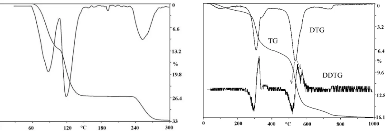
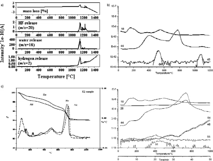
Figure 1. Formalized DTA curve . . . . Figure 2. Formalized TG curve . . . . Figure 3. Determination of peak resolution . . . . Figure 4. TG curve of calcite (Triassic limestone, Gerecse Mts, Hungary) . . . . Figure 5. TG base line and TG curves of CuSO4⋅5H2O (after BALCEROVWIAK1988) . . . . Figure 6. TG and DTG curves of the dehydration of CuSO4⋅5H2O . . . . Figure 7. Separation of the overlapped reactions of boehmite and kaolinite by DDTG (bauxite, Nyirád, Hungary) Figure 8. Separation of the overlapped reactions of boehmite and kaolinite by Q-DTG (bauxite, Nyirád, Hungary) Figure 9. Separation of the overlapping reactions of kaolinite and siderite by thermo-gas-titrimetric determination of siderite . . . . Figure 10. a)DEGAS — thermogravimetry in vacuum and release of CO2, water and hydrocarbons of a kaoline from Washington County, b) TG-DTG plot of a kaolin sample (K2) in He and air at a heating rate of 20 °C min–1(after CARLEERet al. 1998), c) Ion-chromatograms (GC-MS) of gases released by heating of the same sample above in air, below in He as a function of temperature (after CARLEERet al. 1998) . . . . Figure 11. Calculation of virtual kinetic parameters from T, TG and DTG curve . . . . Figure 12. PA curve of well-ordered kaolinite from Mesa Alta (based on data measured by SMYKATZ-KLOSS1974) Figure 13. Indirect parameters for the characterisation of materials . . . . Figure 14. Quarry sap on bentonite sample (from Buru, Romania) and the same sample 4 months later . . . . Figure 15. Q-TG curve of Na-montmorillonite . . . . Figure 16. Dehydration of Cs-montmorillonite . . . . Figure 17. Dehydration of K-montmorillonite . . . . Figure 18. Dehydration of sodium activated montmorillonite . . . . Figure 19. Dehydration of Ag-montmorillonite . . . . Figure 20. DTG curve of the two-step dehydration of Li-montmorillonite . . . . Figure 21. IR spectra of Li-montmorillonite samples in OH stretching regions: unheated and after heating for 24h at 300 °C. (after MADEJOVÁet al. 1999) . . . . Figure 22. DTG and DDTG curves of Ba-montmorillonite dehydration . . . .
128 128 128 129 129 130 130 130 130 130 131 131 131 132 132 133 133 133 134 134 134 134 135 135 135 136 136 137 138 141 177
18 18 20 22 23 23 23 23 24
25 25 26 26 29 30 30 31 31 31 31 31 32
8
Figure 23. DTG and DDTG curves of Hg-montmorillonite dehydration . . . . Figure 24. DTG curve of dehydration of Ca-montmorillonite (Kuzmice, Slovakia) . . . . Figure 25. DTG and DDTG curves of dehydration of Ca-montmorillonite (Egyházaskesző, Hungary) . . . . Figure 26. Interlayer cation contents of smectites in the samples from Hole 735B of Ocean Drilling Program (after ALT, BACH2001) . . . . Figure 27. Thermoanalytical curves of fresh Mn-montmorillonite . . . . Figure 28. Thermoanalytical curves of the same Mn-montmorillonite three years later . . . . Figure 29. DTG curve of dehydration of Mg-montmorillonite . . . . Figure 30. DTG curve of dehydration of Al-montmorillonite . . . . Figure 31. DTA curves of dehydration of Al-montmorillonite treated with solutions of various pH values (after MAFTULEACet al. 2002) . . . . Figure 32. Dehydration temperature and “PA curve” of montmorillonites based on the measurement of 382 different natural samples . . . . Figure 33. Dehydration temperature and “PA curve” of illites and glauconites . . . . Figure 34. Dehydration temperature and “PA curve” of different kind of zeolites . . . . Figure 35. Q-TG curve of mordenite . . . . Figure 36. TG and DTG curves of perlite (Lehotka, Slovakia) . . . . Figure 37. DTG and TG curves of perlite series in Borehole Kishuta–1 . . . . Figure 38. PA curve of opals . . . . Figure 39. Decrepitation of barite (open crucible, curve 1) . . . . Figure 40. Evolution of water bound as solid solution from aragonite . . . . Figure 41. Dehydration of CuSO4⋅5H2O examined by dynamic (curves 1–2) and “quasi-isothermal” (curve 3) heat- ing techniques using open and labyrinth crucibles . . . . Figure 42. Dehydration of MgSO4⋅7H2O examined by dynamic (curves 1–2) and “quasi-isothermal” (curve 3) heat- ing techniques using open (curves 1–2) and labyrinth crucibles (curve 3) . . . . Figure 43. Dehydration of gypsum (CaSO4⋅H2O) under dynamic heating . . . . Figure 44. Dehydration of gypsum (CaSO4⋅H2O) under “quasi-isothermal” and “quasi-isobaric” conditions . . . . . Figure 45. PA curves of the first and the second reaction of water escape from gypsum . . . . Figure 46. (001) projection of the unit cell of palygorskite (BRADLEY1940) . . . . Figure 47. PA curves of the different water types in palygorskite . . . . Figure 48. TG, DTG, and DTA curves of colemanite (WACŁAWSKAet al. 1988) . . . . Figure 49. Decomposition temperature versus electronegativity . . . . Figure 50. Comparison of the decomposition temperature of single and double carbonates . . . . Figure 51. H2- and H2O-release from standard kaolinite KGa–1, Georgia, USA . . . . Figure 52. Q-TG curve of portlandite . . . . Figure 53. Q-TG curve of calcite . . . . Figure 54. TG and DTG curve of chalcanthite under dynamic heating (a), TG curve of chalcanthite under quasi-stat- ic circumstances (b) . . . . Figure 55. Q-TG curves of dehydroxylation processes of boehmite, kaolinite and pyrophyllite. . . . . Figure 56. TG and DTG curve of mixture of calcite and dolomite . . . . Figure 57. TG curve of mixture of dolomite and calcite under quasi-static circumstances . . . . Figure 58. Aluminite Borehole Csordakút–421, 38.2–38.3 m (Hungary) . . . . Figure 59. Calcite impurities in an aluminite sample Borehole Csordakút–421, 38.8–38.9 m (Hungary) . . . . Figure 1.1. Thermoanalytical curves of sulphur . . . . Figure 1.2.1. Graphite oxidation in air . . . . Figure 1.2.2. Graphite oxidation in oxygen (DTA, TG, DTG, TGT and DDTG curves) . . . . Figure 2.1.1. DTA, TG and DTG curves of the complex reactions of a sample with relatively high pyrite content Figure 2.1.2. DTA, TG and DTG curves of the oxidation of pyrite in oxygen . . . . Figure 2.1.3. DTA, TG and DTG curves of the disproportion of pyrite in nitrogen . . . . Figure 2.2. Oxidation and sublimation of cinnabar . . . . Figure 2.3. Thermoanalytical curves of galena . . . . Figure 2.4. Thermoanalytical curves of sphalerite . . . . Figure 3.1.1. Thermoanalytical curves of quartz . . . . Figure 3.1.2. Thermoanalytical curves of opal . . . . Figure 3.2.1. Oxidation reaction of magnetite . . . . Figure 3.2.3a. Surface structural model for ferrihydrite. (MANCEAU, GATES1995) . . . . Figure 3.2.3b. Derivatogram of ferrihydrite . . . . Figure 3.3.1. Derivatogram of pyrolusite . . . . Figure 4.1.1a. Thermogravimetric curves of natural gibbsite . . . . Figure 4.1.1.b. PA curve of natural gibbsite . . . . Figure 4.1.1c. Thermogravimetric curves of artifical gibbsite . . . .
32 32 32 33 33 33 33 34 35 35 35 36 36 37 37 37 37 38 38 39 39 39 39 40 40 40 41 41 41 42 42 42 43 43 43 46 46 48 48 49 49 52 52 53 53 54 54 56 56 57 58 59 60 61 61
Figure 4.1.2. Thermogravimetric curves of a sample containing nordstrandite . . . . Figure 4.1.3. Thermogravimetric curves of a sample containing brucite . . . . Figure 4.1.4. Thermogravimetric curves of a sample containing portlandite . . . . Figure 4.2.1a. Thermogravimetric curves of a sample containing goethite . . . . Figure 4.2.1b. Temperature of dehydration peak, the shift of d111X-ray reflection and the wawe number of the defor- mation band around 900 cm–1as function of the aluminium content of goethite (after JÓNÁS, SOLYMÁR1970b) . . Figure 4.2.1c. Thermogravimetric curves of a sample containing alumo-goethite . . . . Figure 4.2.2. Thermogravimetric curves of a sample containing lepidocrocite . . . . Figure 4.2.3. Thermogravimetric curves of a sample containing manganite . . . . Figure 4.2.4. Thermogravimetric curves of a sample containing boehmite . . . . Figure 4.2.5a. Thermogravimetric curves of a sample containing diaspore . . . . Figure 4.2.5b. PA curves of Hungarian diaspore and boehmite minerals from bauxite . . . . Figure 4.3.1. Thermogravimetric curves of a sample containing lithiophorite . . . . Figure 5.1.1.1.1a. Thermoanalytical curves of kaolinite . . . . Figure 5.1.1.1.1b. Thermoanalytical parameters used for the determination of the crystalinity of kaolinite from the DTA curve . . . . Figure 5.1.1.1.1c. Indirect parameters for the characterisation of kaolinite . . . . Figure 5.1.1.1.1d. Thermoanalytical parameters used for the the determination of the crystalinity of the kaolinite from the DTG curve . . . . Figure 5.1.1.1.2. Thermoanalytical curves of dickite . . . . Figure 5.1.1.1.3. Thermoanalytical curves of fireclay . . . . Figure 5.1.1.1.4. Thermoanalytical curves of halloysite . . . . Figure 5.1.1.1.5. Thermoanalytical curves of an allophane containing sample . . . . Figure 5.1.1.2a. Thermal reaction schemes of reaction sequences of Mg-chrysotile. According to BALL, TAYLOR
(1963), BRINDLEY, HAYAMI(1965), and MARTIN(1977). Summarized by MACKENZIEand MEINHOLD(1994) . . . . . Figure 5.1.1.2b Schematic representation of proposed chrysotile reaction sequences according to MACKENZIE, MEINHOLD(1994). . . . Figure 5.1.1.2c. Thermoanalytical curves of chrysotile . . . . Figure 5.1.1.2d. Thermoanalytical curves of lizardite . . . . Figure 5.1.1.2e. Thermoanalytical curves of “hydroantigorite” . . . . Figure 5.1.2.1.1. Thermogravimetric curves of pyrophyllite . . . . Figure 5.1.2.1.2. Thermogravimetric curves of a talc containing sample . . . . Figure 5.1.2.2.1.1a. Typical thermogravimetric curves of primary Ca-montmorillonite . . . . Figure 5.1.2.2.1.1b. Derivatogram of sample containing montmorillonite . . . . Figure 5.1.2.2.1.1c. Quantitative determination using ethylenglycole . . . . Figure 5.1.2.2.1.2. Typical thermogravimetric curves of primary Na-montmorillonite . . . . Figure 5.1.2.2.1.3a. Thermogravimetric curves of an “abnormal montmorillonite” with double dehydroxylation . . Figure 5.1.2.2.1.3b. Thermogravimetric curves of an “abnormal montmorillonite” with a low temperature dehydrox- ylation . . . . Figure 5.1.2.2.1.3c. DTA curve of a Wyoming-type montmorillonite . . . . Figure 5.1.2.2.1.3d. DTA curve of a Cheto-type montmorillonite . . . . Figure 5.1.2.2.2. Thermogravimetric curves of iron beidellite . . . . Figure 5.1.2.2.3. Thermogravimetric curves of nontronite . . . . Figure 5.1.2.2.4a. Thermogravimetric curves of saponite . . . . Figure 5.1.2.2.4b. Thermogravimetric curves of iron-saponite . . . . Figure 5.1.2.3. Thermoanalytical curves of vermiculite . . . . Figure 5.1.2.4.1a. Unpulverised sample containing muscovite . . . . Figure 5.1.2.4.1b. Effects of dry grinding on muscovite . . . . Figure 5.1.2.4.1c. Thermogravimetric curves of same muscovite pulverised under methanol . . . . Figure 5.1.2.4.2a. Thermogravimetric curves of fresh biotite . . . . Figure 5.1.2.4.2b. Signal of the initial chloritization of a biotite separate. . . . . Figure 5.1.2.5.1. Thermogravimetric curves of illite containing sample . . . . Figure 5.1.2.5.2. Thermogravimetric curves of a hydromuscovite containing sample . . . . Figure 5.1.2.5.3. Thermogravimetric curves of a glauconite separate . . . . Figure 5.1.2.6a. Typical thermoanalytic curves of primary chlorite . . . . Figure 5.1.2.6b. Typical thermoanalytic curves of sedimentary chlorite . . . . Figure 5.1.2.7.1.1. Thermoanalytic curves of K-rectorite (allevardite) . . . . Figure 5.1.2.7.1.3. Thermoanalytic curves of tosudite . . . . Figure 5.1.2.7.2.1. Thermoanalytic curves of interstratified illite/montmorillonite . . . . Figure 5.1.2.7.2.2. Thermoanalytic curves of interstratified chlorite-vermiculite . . . . Figure 5.1.2.7.2.3. Thermoanalytic curves of interstratified talc-saponite . . . .
62 63 63 64 64 64 65 65 66 66 66 67 68 69 69 70 70 70 71 71 73 73 73 74 74 75 76 77 77 77 78 78 79 79 79 80 80 80 81 81 82 82 82 83 83 84 84 84 85 85 86 86 87 87 87
10
Figure 5.1.2.8.1. Thermogravimetric curves of a palygorskite-bearing sample . . . . Figure 5.1.2.8.2. Thermoanalytic curves of sepiolite . . . . Figure 5.1.2.9.1. Thermoanalytic curves of apophyllite . . . . Figure 5.1.2.9.2. Thermoanalytic curves of prehnite . . . . Figure 5.1.2.9.3. Thermoanalytic curves of tobermorite . . . . Figure 5.2.1. Thermoanalytic curves of a topaz-bearing sample . . . . Figure 5.2.2. Thermogravimetric curves of an epidote-bearing sample . . . . Figure 5.2.3. Thermoanalytic curves of a vesuvianite-bearing sample . . . . Figure 5.2.4. Thermoanalytic curves of a zunyite-bearing sample . . . . Figure 5.2.5. Thermogravimetric curves of katoite . . . . Figure 5.3.2. Thermogravimetric curves of ferroaxinite . . . . Figure 5.3.3. Thermoanalytical curves of a tourmaline (dravite)-bearing sample . . . . Figure 5.4.2. Thermogravimetric curves of charoite . . . . Figure 5.5.1.1.1. Thermogravimetric curves of natrolite . . . . Figure 5.5.1.1.4. Thermoanalytic curves of a thomsonite-bearing sample with gonnardite? impurities . . . . Figure 5.5.1.2.1. Thermogravimetric curves of analcime . . . . Figure 5.5.1.2.2. Thermoanalytical curves of laumontite (leonhardite?) . . . . Figure 5.5.1.3.2. Thermogravimetric curves of phillipsite . . . . Figure 5.5.1.4.1. Thermogravimetric curves of mordenite . . . . Figure 5.5.1.5.2. Thermogravimetric curves of clinoptilolite . . . . Figure 5.5.1.5.3. Thermoanalytical curves of stilbite . . . . Figure 5..5.1.6.3. Thermoanalytical curves of chabasite . . . . Figure 6.1.1a. Thermogravimetric curves of calcite . . . . Figure 6.1.1b. Thermogravimetric curves of a strongly weathered calcite . . . . Figure 6.1.2. Thermogravimetric curves of magnesite . . . . Figure 6.1.3. Thermogravimetric curves of rhodochrosite . . . . Figure 6.1.4a. Thermoanalytical curves of siderite . . . . Figure 6.1.4b. Superposition of the endothermic and exothermic reactions on the DTA curve of siderite . . . . Figure 6.1.5. Thermoanalytical curves of cerussite . . . . Figure 6.2.1a. Thermogravimetric curves of dolomite . . . . Figure 6.2.1b. Thermogravimetric curves of dolomite in loess . . . . Figure 6.2.1c. Thermogravimetric curves of dolomite in palaeosoil . . . . Figure 6.2.1d. Thermogravimetric curves of “protodolomite” (Mg-poor dolomite) bearing rock with halite content Figure 6.2.1e. Thermogravimetric curves of the previous sample after washing by distilled water . . . . Figure 6.2.1f. Thermogravimetric curves of high magnesium calcite and Ca-dolomite (“protodolomite”) . . . . Figure 6.2.2. Thermogravimetric curves of huntite . . . . Figure 6.2.3. Thermoanalytical curves of real ankerite . . . . Figure 6.2.4a. Thermogravimetric curves of ferrous dolomite with higher iron content . . . . Figure 6.2.4b. Thermogravimetric curves of ferrous dolomite . . . . Figure 6.2.4c. Thermogravimetric curves of ferrous dolomite with low iron content . . . . Figure 6.2.5. Thermogravimetric curves of kutnahorite . . . . Figure 6.3.1. Thermoanalytical curves of kalicinite . . . . Figure 6.3.2. Thermogravimetric curves of teschemacherite . . . . Figure 6.4.1. Thermogravimetric curves of malachite . . . . Figure 6.4.3. Thermoanalytical curves of dawsonite . . . . Figure 6.5.1. Thermogravimetric curves of dypingite . . . . Figure 7.1.1. Thermoanalytical curves of a mascagnite bearing sample . . . . Figure 7.2.1.Thermogravimetric curves of chalcanthite . . . . Figure 7.2.2. Thermoanalytical curves of melanterite . . . . Figure 7.2.3. Thermoanalytical curves of rozenite . . . . Figure 7.2.4. Thermoanalytical curves of szomolnokite bearing sample . . . . Figure 7.2.5. Thermogravimetric curves of alunogen . . . . Figure 7.2.6. Thermogravimetric curves of hexahydrite . . . . Figure 7.2.7. Thermogravimetric curves of a gypsum bearing sample . . . . Figure 7.3.1. Thermoanalytical curves of römerite . . . . Figure 7.3.2. Thermogravimetric curves of voltaite . . . . Figure 7.3.3. Thermoanalytical curves of halotrichite . . . . Figure 7.3.4. Thermogravimetric curves of potassium-alum . . . . Figure 7.3.5. Thermogravimetric curves of tschermigite . . . . Figure 7.4.1. Thermoanalytical curves of alunite . . . . Figure 7.4.2. Thermoanalytical curves of a jarosite bearing sample . . . .
88 89 89 90 90 91 91 92 92 93 93 94 95 96 97 99 100 101 102 103 104 106 108 108 109 109 110 110 111 111 112 112 113 113 113 113 114 114 115 115 115 116 116 117 117 118 122 122 123 123 124 124 125 125 125 126 126 127 127 128 128
Figure 7.5.1. Thermoanalytical curves of an aluminite bearing sample . . . . Figure 7.5.3. Thermoanalytical curves of copiapite . . . . Figure 8.1.1. Thermoanalytical curves of vivianite . . . . Figure 8.2.1. Thermoanalytical curves of lazulite . . . . Figure 8.2.2. Thermoanalytical curves of gorceixite . . . . Figure 8.3.1. Thermoanalytical curves of diadochite . . . . Figure 8.4.1. Thermoanalytical curves of kaňkite . . . . Figure 10.1a. Thermoanalytical curves of halite . . . . Figure 10.1b. Thermoanalytical curves of an admixture of epsomite and halite . . . . Figure 11.1. Thermoanalytical curves of whewellite . . . . Figure 11.2. Thermoanalytical curves of humboldtine . . . . Figure 12.1. DTA curves of 20 mg coal sample diluted by 980 mg Al2O3 . . . . Figure 12.2. Characterisation of coal by thermogravimetric analysis . . . . Figure 13.1. Thermogravimetric curves of perlite . . . . Figure 13.2. Quantitative evaulation of a bauxite sample . . . . Figure14.6b. Wheathering (palaeoclimate ) curve of a loess section in Borehole Üveghuta–22 (Hungary), based on the molecular and hydroxid water content measured from TG curves. . . . . Figure 14.7. Relationship between the interlayer water content and the metasomatic alteration temperature in the Borehole Pázmánd–2, Hungary . . . . Figure 14.8a. Characteristic thermal decomposition temperature for kaolinite of different genesis compared to Mesa Alta kaolinite . . . . Figure 14.8b. Characteristic thermal parameters for kaolinite of different diagenetic stage compared to hydrothermal kaolinite . . . . Figure 14.8c. Peak temperature of exothermic reaction for kaolinite of different genesis . . . . Figure 14.12a. δ13C and δ18O values . . . . Figure 14.12b. Corrected decomposition temperature of travertine sample from different locallities . . . .
Index of Tables
Table 1. Individual thermoanalytical techniques . . . . Table 2. Dimensions of thermoanalytical parameters (the recommended SI symbols should be used) . . . . Table 3. Conventions of recording . . . . Table 4. Empirical parameters for the description of peak shape . . . . Table 5. Available Certified Reference Materials . . . . Table 6. Proposed standard conditions of the thermoanalytical investigation of minerals (by SMYKATZ-KLOSS1974) Table 7. Proposed standard conditions of the treatment (by SMYKATZ-KLOSS1974) . . . . Table 8. Schema of thermo-gas-titrimetric determination of different components . . . . Table 9. Joint use of instrument-based mineralogical phase analytical methods (DTA-TG, XRD, IR) . . . . Table 10. Chemical and physical thermal reaction types and their appearance on thermoanalytical curves . . . . Table 11. The most frequent types of occurrence of water in minerals and their most characteristic thermoanalytical features . . . . Table 12. Measurement parameters of the bentonite sample from Buru, Romania . . . . Table 13. Hydration enthalpies (∆Hhyd) of metal cations . . . . Table 14. Characteristic data of the monovalent and bivalent interlayer cations. . . . . Table 15. Probable state of active centres of Al-montmorillonite treated with solutions of various pH values. . . . Table 16. Temperature of decomposition depending on the electonegativity . . . . Table 17. Temperature of decomposition of hydroxide in different types of structures depending on the electronega- tivity . . . . Table 18. Characteristic evaporation and sublimation temperature of minerals . . . . Table 19. Characteristic temperatures of the oxidation and the reduction of minerals . . . . Table 20. Types of solid-phase structural decomposition and crystallization of new phases . . . . Table 21. Characteristic temperatures of polymorphic transition of minerals . . . . Table 22. Characteristic melting points of minerals . . . . Table 23. Curie point of minerals . . . . Table T2a. Oxidation of the most common simple sulphide minerals in order of temperature (°C) . . . . Table T2b. Principal modes of oxidation of pyrite . . . . Table T2c. Further reactions of sulphides. . . . Table T3.1. Thermal reactions of silica minerals . . . . Table T3.2.3. DTA reaction of synthetic iron oxide gels . . . . Table T3.3.2. Thermal reactions of other manganese oxides . . . . Table T4.1. Dehydroxylation process of simple hydroxide minerals . . . .
128 129 130 131 131 132 132 133 133 134 135 135 136 136 137 138 139 139 139 140 140 140
16 18 18 19 19 21 21 24 27 28 28 29 30 33 34 40 42 43 43 44 44 45 46 50 50 51 55 59 60 61
Table T.4.2. Dehydroxylation of oxyhydroxide minerals . . . . Table T5.1.1. Thermoanalytical data of 1:1 layer type clay minerals . . . . Table T5.1.1.1a, b. Characterisation of kaolinite types based on different DTA parameters . . . . Table T5.1.1.2a. Characteristic peak temperatures of Mg-serpentines based on different references . . . . Table T5.1.1.2b. Temperature interval data of Mg-serpentines . . . . Table T5.1.2. Thermoanalytical data of the main 2:1 layer type clay minerals . . . . Table T5.1.2.5. Composition of the members of the muscovite-illite series . . . . Table T5.1.2.6. Thermoanalytical data of the main 2:1:1 layer type phyllosilicates . . . . Table T5.1.2.8.1. Dehydration temperature of water evaluated from palygorskite on the basis of published data . . Table T5.1.2.8.2. Steps of the water escape from sepiolite based on published data . . . . Table T5.2. Dehydroxylation temperature of some mesosilicates . . . . Table T5.5.1.1.1. Thermoanalytical data of natrolite . . . . Table T5.5.1.1.2. Thermoanalytical data of gonnardite . . . . Table T5.5.1.1.3. Thermoanalytical data of mesolite . . . . Table T5.5.1.1.4. Thermoanalytical data of thomsonite . . . . Table T5.5.1.1.5. Thermoanalytical data of scolecite . . . . Table T5.5.1.1.6. Thermoanalytical data of edingtonite . . . . Table T5.5.1.2.1. Thermoanalytical data of analcime . . . . Table T5.5.1.2.2. Thermoanalytical data of laumontite . . . . Table T5.5.1.3.1. Thermoanalytical data of gismondine . . . . Table T5.5.1.3.2. Thermoanalytical data of phillipsite . . . . Table T5.5.1.3.3. Thermoanalytical data of harmotome . . . . Table T5.5.1.4.1. Thermoanalytical data of mordenite . . . . Table T5.5.1.5.1. Thermoanalytical data of heulandite . . . . Table T5.5.1.5.2. Thermoanalytical data of clinoptilolite . . . . Table T5.5.1.5.3. Thermoanalytical data of stilbite . . . . Table T5.5.1.6.1. Thermoanalytical data of gmelinite . . . . Table T5.5.1.6.2. Thermoanalytical data of erionite . . . . Table T5.5.1.6.3. Thermoanalytical data of chabasite . . . . Table T5.5.1.6.4. Thermoanalytical data of faujasite . . . . Table T5.5.1.7. Thermoanalytical data of other zeolites . . . . Table T6.1a. The most important reactions of simple carbonate minerals . . . . Table T6.1b. Further reactions of simple carbonates . . . . Table T6.2. The main reactions of double carbonate minerals . . . . Table 6.2.1. Composition of carbonate in loess and palaeosoil analysed by different methods . . . . Table T6.5.1. Thermal reactions of nesquehonite . . . . Table 6.5.2. Thermal reactions of hydromagnesite . . . . Table T6.5.4. Thermal reactions of hydrotalcite . . . . Table T6.6. Thermal reaction of other carbonates according to data of BECK(1950) . . . . Table T7a. The main reactions of the most frequent simple sulphate minerals . . . . Table T7b. Further reactions of sulphates . . . . Table T7.1.1. Reaction of mascagnite according to the literature . . . . Table T12.2. Characterisation of coal by thermogravimetric analysis . . . . Table T13.2a. Evaluation by the measured data . . . . Table T13.2b. Comparison the results of different investigations . . . . Table T14.8. Characteristic thermal parameters of crystallinity for kaolinite of different genesis . . . .
12
64 68 69 72 72 74 83 85 88 89 91 95 96 96 97 98 98 98 99 100 101 101 102 102 103 104 105 105 105 106 106 107 108 111 112 117 118 118 119 121 121 122 136 137 137 139
Thermal analysis plays a specific role in the identification and quantitative determination of mineral components of rocks. In spite of the fact that minerals were the first group of materials studied regularly by using thermoanalytical meth- ods, the potential offered by these methods is still not fully utilized in the field of earth sciences. The range of thermoana- lytical methods applied in earth sciences is rather wide. Most works are based on DTA. DTA data provide indirect analyt- ical information on a material and the quantification of a reaction is limited. From quantitative phase analysis point of view it is very important that thermogravimetric measurements give direct and absolute values for thermal reactions making sto- ichiometric calculation possible. Both DTA (Differential Thermal Analysis) and TG (Thermogravimetry) are undoubtedly the most widespread methods, whereas the rest are normally applied rather occasionally, to find solution to specific prob- lems only.
Thermogravimetry dates back to the work of TALABOTwho in 1833 equipped a laboratory with thermobalances for qual- ity control of Chinese silk. Thermogravimetric analysis of the minerals and rocks has been applied systematically since the mid 1960s. Derivatography, the technique of simultaneous thermal analytical measurement developed by PAULIKs was a combination of TG and DTA. The measure the rate of change of the sample property with temperature, later the sample controlled thermal analysis or controlled rate thermal analysis (quasi-thermogravimetry) and the computerized new gener- ation of these equipments received the possibility to the author during 40 years to analyze about 30 000 geological samples.
The experiences of this long time permit of the systematization of the thermal reactions of the minerals and made reason- able the compilation of this book. Handbook for geological samples based on thermogravimetry earlier only the otherwise excellent publication by TODORin 1972.
Mária FÖLDVÁRI
PREFACE
MEASUREMENT METHODS AND SYSTEM OF
THERMAL REACTIONS OF MINERALS
INTRODUCTION TO THE THERMOANALYTICAL METHODS
The International Confederation for Thermal Analysis and Calorimetry has published several recommendations for the nomenclature, standardizing and publishing of results of thermal analysis.
Thermoanalytical techniques
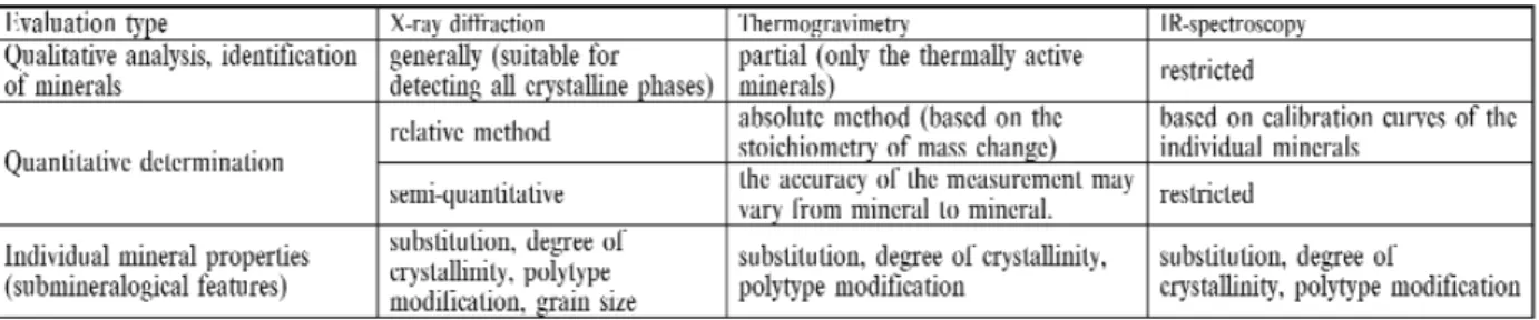
Thermal analysis is a group of analytical techniques in which physical properties or chemical reactions of a substance are measured as a function of temperature. The classification of the individual thermoanalytical techniques are summarised in Table 1.
Differential thermal analysis (DTA)
A technique in which the temperature difference between a substance and a reference material is measured as a func- tion of temperature whilst the substance and reference material are subjected to the same controlled temperature pro- gramme.
Table 1. Individual thermoanalytical techniques
The technique requires the use of a reference material, which is a known substance, usually inactive thermally (inert material) over the temperature range interest. Important features of the reference material are that the thermal characteris- tic (specific heat, conductivity etc.) and the particle size should be very similar to that of the sample.
The most commonly used reference materials:
— calcined α-Al2O3,
— calcined MgO,
— a part of the of the sample precalcined to 1000 °C,
— calcined quartz-free kaolinite,
— quartz.
Thermogravimetry (TG)
A technique in which the mass of a substance is measured as a function of temperature while the substance is subject- ed to a controlled temperature programme.
Evolved Gas Analysis (EGA)
A technique in which the nature and/or amount of volatile product(s) released by a substance are/is measured as a func- tion of temperature whilst the substance is subjected to a controlled temperature programme.
Derivative technique
The derivative technique yields the first derivative of the original thermal curve with the respect to either time or tem- perature. It may be possible to measure the rate of property change. These curves give a higher resolution and present more accurately the specific temperature characteristics. The derivative curves obtained by using different instrumental tech- niques or by computerized derivation. If necessary the second derivative of the primary curves may also be displayed by deriving (e.g. TG
DTG
DDTG or DTA
DDTA).Multiple techniques
— Simultaneous techniques: application of two or more techniques to the same sample at the same time (e.g. simulta- neous thermogravimetry and differential thermal analysis in derivatograph).
— Coupled simultaneous techniques: application of two or more techniques to the same sample when two instruments are connected through an interface (e.g. differential thermal analysis and mass spectrometry).
— Combined techniques: application of two or more techniques using separate samples for each technique.
Experimental conditions
Thermal measurements can be carried out:
1. With different heating techniques:
a) Under dynamic temperature change:
— heating:
— linear or constant rate e.g. temperature/time curve is linearly programmed.
— cooling:
— according to heat-incapacity of the furnace,,
— programmed (cooling rate less than the heat-incapacity of the furnace).
b) Under static conditions:
— isothermal,
— quasi isothermal (at a quasi equilibrium condition i.e. self regulation by the constant partial pressure of the volatile products, Q-TG, Q-DTG, Q-DTA etc.),
— special quasi isothermal (at a quasi equilibrium condition combined by timing).
c) Combined.
2. Under different types of gas atmosphere: air, oxygen, nitrogen, argon, helium (20% O2, 80% He) or in vacuum.
Thermoanalytical parameters
The following tables summarise the principles of the most important definitions which are used in earth sciences and in this book (Table 2, 3).
17
Nomenclature of DTA and TG curves
A formalized DTA curve is shown in Figure 1.
Base line: AB and DE correspond to the portion or portions of the DTA curve for which ∆T is approximately zero.
Peak: BCD is that portion of the DTA curve which departs from and subsequently returns to the base line.
Initial temperature: B (characteristic reaction temperature) deter- mination is approximate
Final temperature: D (the sample again has the same temperature as the inert material, ∆T = 0).
Peak temperature: point of intersection of CF and the temperature axis (maximum rate of reaction) can be measured quite accurately.
Endothermic peak: is a peak where the temperature of the sample falls below that of the reference material (∆T is negative).
Exothermic peak: is a peak where the temperature of the sample rises above that of the reference material (∆T is positive).
Peak width (reaction temperature range): B’D’ is the time or tem- perature interval between the points of departure from and return to the base line.
Peak width at half height: reaction width at ∆T/2.
Peak height: CF is the distance vertical to the time or temperature axis, between the interpolated base line and the peak tip.
Peak area: BCDB is the area enclosed between the peak and the interpolated base line. There are several ways to inter- polate the base line. (Later Figure 6 gives only an example.) Locations of B and D depend on the method of interpolation of the base line (reaction heat DH).
Extrapolated onset: G is the point of intersection of the tangent drawn at the point of greatest slope on the leading edge of the peak (BC) with the extrapolated base line.
Base line of DTA curve is where ∆T is zero.
Base line shift: γdifference between the specific heat of the orig- inal sample and its reaction product.
All definitions refer to a single peak such as that shown in Figure 1; multiple peak system, showing shoulders or more than one maxi- mum or minimum, can be considered to result from the superposition of single peaks.
While the true characteristic reaction temperature can be deter- mined only approximately, the peak temperature can be measured quite accurately.
Table 2. Dimensions of thermoanalytical parameters (the recommended SI symbols should be used)
Table 3. Conventions of recording
Figure 1. Formalized DTA curve
Figure 2. Formalized TG curve
A formalized TG curve is shown in Figure 2.
Plateau: AB is that part of the TG curve where the weight is essentially constant.
Initial temperature (Ti) B is the temperature (on the Celsius or Kelvin scales) at which the cumulative weight reaches a magnitude that the thermobalance can detect.
Final temperature (Tf) C is the temperature (on the Celsius or Kelvin scales) at which the cumulative weight reaches a maximum.
The reaction interval is the temperature difference between Tf and Tias defined above.
All definitions refer to a single-step process, multistage processes can be considered as resulting from a series of single- step processes.
Description of the shape of thermoanalytical curves (DTA, DTG)
Parameters (Table 4) characterize the four empirical properties of a peak:
1. position of the peak along the temperature axis: such as T(max), T(α) 2. width: ∆T(α2,a1), WT,
3. asymmetry: a(max), R(α)etc.
4. sharpness/flatness of the peak: U etc.
Form: shoulder.
Calibration
The apparatus should be calibrated before starting investigations and later after almost 200 runs.
Temperature and DTA calibration
Based on the recommendation of ICTA (International Confederation for Thermal Analysis) Committee on Standardization solid I
"
solid II first order phase transitions would be preferable for use in dynamic DTA (Table 5).19
Table 4.Empirical parameters for the description of peak shape
Table 5.Available Certified Reference Materials
*National Bureau of Standards
Evaluation of DTA peak resolution
4:1 mixture (by weight) of SiO2and K2SO4
∆T/dt 10 °Cmin–1 Reactions:
1. at 574 °C: transition of α-quartz
β-quartz,2. at 583 °C: transition of K2SO4 rhombic
K2SO4 hexagonal value of the resolution:where x = the height of SiO2peak,
y = the minimum deviation the experimental curve from the base-line in region between the peaks.
Other materials usually used for calibration
Heat of reaction (∆H)
C12H22O11 (sacharose = cane sugar) during the reaction: C12H22O11+12O2
12CO2+11H2O.During the reaction the combustion heat (peak area) 16.51 joule/mg.
TG calibration
KHCO3at 170 °C (heating rate: 5 Kmin–1) KHCO3
CO2+H2O+K2CO3. Theoretical mass loss based on the reaction is 31%.DTG calibration
Total evaporation of methanol (CH3OH).
Effects influencing thermoanalytical curves
In thermal analysis the influence of all the apparative and preparative factors is much greater than in other mineralogi- cal techniques (e.g. X-ray method):
1. Experimental conditions
— Apparative factors:
— heating rate (with increasing heating rate peak temperature shifts higher and,
— shape of DTA peak also changes),
— sample arrangement,
— furnace atmosphere,
— shape of crucible,
— thermocouple, etc.
— Preparation:
— packing density,
— grain size,
— amount of the sample,
— humidity of the air in the laboratory (dehydration of clay minerals), etc.
2. Properties of the substance
Reasons of the drift of base line in DTA curves:
— differences in heat conductivity and heat capacity of the sample and inert substance (partial elimination: mixing the sample with inert material or reducing the sample amount),
— difference between the specific heat of the original sample and its reaction product,
— imperfect centring of the sample holder in the furnace.
Figure 3.Determination of peak resolution
percent resolution = ,
21
Standardization
Consequences of influencing experimental conditions: As much as possible the mineralogical thermoanalytical investi- gation should be made under standard conditions (Table 6 and 7) to get comparable and reproducible results.
In the case of investigating a series of similar samples it is absolutely necessary to analyse always under the same conditions.
Each published thermoanalytical curve should be completed by the information on all conditions of the analysis.
Recommendations of ICTA Nomenclature Committee for reporting thermal analysis results
— Identification of all substances (sample, reference, diluent) by a definitive name, an empirical formula, or equivalent compositional data.
— The origin of all substances, details of their histories, pre-treatment and chemical purities, so far as these are known.
— Measurement of the average rate of linear temperature change over the temperature range involving the phenomena of interest. Non-linear temperature programming should be described in detail.
— Identification of the sample atmosphere by pressure, composition and purity; whether the atmosphere is static, self-gener- ated, or dynamic through or over the sample. Where applicable, the ambient atmospheric pressure and humidity should be spec- ified. If the pressure is other than atmospheric, full details of the method of control should be given.
— A statement of the dimensions, geometry and material of the sample holder (open, closed).
— A statement of the method of loading (quasi-static, dynamic) where applicable.
— Identification of the abscissa scale in terms of time or of temperature at a specific location. Time or temperature should be plotted to increase from left to right.
— Information about the methods applied to identify intermediates or final products.
— Faithful reproduction of all origin records.
— Identification of the apparatus used by type and/or commercial name The following additional details are also necessary in the report of DTA data:
— Wherever possible, each thermal effect should be identified and supplementary supporting evidence stated.
— Sample weight and dilution of the sample, particle size.
— Use of grinding apparatus, size fractionation methods.
— Geometry and materials of the thermocouples and the location of the differential and temperature-measuring ther- mocouples.
— The ordinate scale should indicate deflection per degree Centigrade at a specified temperature. Preferred plotting will indicate upward deflection as a positive temperature differential, and downward deflection as a negative temperature differ- ential, with respect to the reference. Deviations from this practice should be clearly marked.
The following additional details are also necessary in the report of TG data:
— A statement of the sample weight and weight scale for the ordinate. Weight loss should be plotted as a downward trend and deviation from this practice should be clearly marked. Additional scales (e.g. fractional decomposition, molecu- lar composition) may be used for the ordinate when desired.
— If derivative thermogravimetry is employed, then method of obtaining the derivative should be indicated and the units of the ordinate specified.
The following additional details are also necessary in the report of each EGA or EGD record:
— Method (MS, GC, specific detector).
— Interface (time delay, trapping).
— A clear statement of the temperature environment of the sample during reaction.
— Identification of the ordinate scale in specific terms where possible. In general, increasing concentration of evolved gas should be plotted upwards. Deviations from these practices should be clearly marked.
Data acquisition and manipulation by computers:
— How many bits A/D conversion?
— It should be possible to view the raw data prior to any smoothing.
Table 6.Proposed standard conditions of the thermoanalytical investiga- tion of minerals (by SMYKATZ-KLOSS1974)
Table 7. Proposed standard conditions of the treatment (by SMYKATZ- KLOSS1974)
— Equations used in the derivation of properties need to be either given in the handbook or references to the literature are required. An example is the form of the equation used in kinetic analysis.
— How often the signal sampled? How many points are averaged? What base line treatment is actually used?
***
References for thermoanalytical methods: 50, 142, 237, 509, 554, 555, 556, 632, 671, 691, 692, 698, 724, 725, 727, 842, 877, 879, 1006, 1193, 1194
THERMOGRAVIMETRIC INVESTIGATION TECHNIQUES AND METHODS Techniques
Quantitative determination based on mass-change
Quantitative determination methods applied in thermal analysis can be based upon the measurement of DTA peak areas using calibration curves, whereas in the case of decomposition reactions they can be performed by applying the PA (Proben Abhängigkeit = curve of sample amount dependence) curves using the logarithmic relation between the temperature of the decomposition reaction and concentration. However, these methods offer the possibility of semi-quantitative estimation, only. The most suitable methods for quantitative determination are measurements based on mass-changes in the course of decomposition (possibly oxidation and reduction) processes. The advantage of this method is, as compared to any other instrument-based methods of phase analysis, that directly obtained parameters, each with absolute value are used. Within the accuracy range of the analytical balance applied for plotting the TG curves, thermogravimetry may represent one of the most precise analytical methods. Here, from the mass- change in a given reaction, and with the knowledge of ther- mochemical reaction equation the mass percent ratio can be determined for the mineral component in the sample.
The stoichiometric factor introduced for quantitative determination is as follows:
where M = molecular mass of the mineral, m = mass-change during the given reaction.
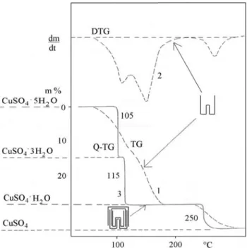
Theoretical thermal reaction of calcite (Figure 4):
CaCO3
CaO+CO2 Molar mass 100 56 44 Stoichiometric factor: 2.27.Calcite content in the sample of Figure 4 = 99%.
Accuracy of determination based on thermogravimetric measurement and the limits of phase detection are different for each mineral. In a multicomponent system the accurate deter- mination of the composition is more difficult than others. For instance, although the weight change of a sample can be found out by means of thermobalance with an accuracy of + 0.1%, the amounts of the individual components of minerals can be determined often only with accuracy lower by several orders of magnitude. This fact attributed to three causes.
The most frequent and difficult problem is caused by the circumstance that the individual mineral components decom- pose closely after one another. Whereas in a favourable case the overlapping of the decomposition only decreases the accu- racy of the determination, under disadvantageous conditions it may totally hinder even the identification of the components.
Theoretically, minerals, for which the stoichiometric factor of the decomposition reaction is the lowest, can be deter- mined with the highest accuracy. For reactions with high stoichiometric factors, the small mass-change and the eventual measurement errors multiplied due to the factor may reduce considerably the accuracy of the measurement and in this case all we can obtain is a semi-quantitative estimation.
In accordance with the above statements, the different minerals can be arranged in the following order:
I. Sublimatory minerals (sulphur, cinnabar) f=1, II. Sulphates (determined from SO3) f=2–6,
Hydroxides (determined from H2O f=1.5–10, Carbonates (determined from CO2) f=2–10, III. Phosphates (determined from H2O) f=2–20,
Zeolites f=4–15,
Phyllosilicates f=7–30,
IV. Certain neso-, soro- and inosilicates f>20.
f = ,
Figure 4. TG curve of calcite (Triassic limestone, Gerecse Mts, Hungary)