fixed boundary or free boundary

On a reaction–diffusion–advection system:

fixed boundary or free boundary

Ying Xu, Dandan Zhu and Jingli Ren

School of Mathematics and Statistics, Zhengzhou University, Zhengzhou 450001, China Received 15 January 2018, appeared 14 May 2018

Communicated by Maria Alessandra Ragusa

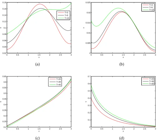
Abstract. This paper is devoted to the asymptotic behaviors of the solution to a reaction–diffusion–advection system in a homogeneous environment with fixed bound- ary or free boundary. For the fixed boundary problem, the global asymptotic stability of nonconstant semi-trivial states is obtained. It is also shown that there exists a stable nonconstant co-existence state under some appropriate conditions. Numerical simu- lations are given not only to illustrate the theoretical results, but also to exhibit the advection-induced difference between the left and right boundaries as time proceeds.

For the free boundary problem, the spreading–vanishing dichotomy is proved, i.e., the solution either spreads or vanishes finally. Besides, the criteria for spreading and van- ishing are further established.

Keywords: reaction–diffusion–advection, fixed boundary, free boundary, nonconstant steady states, spreading–vanishing.

2010 Mathematics Subject Classification: 35Q92, 35K57, 35R35, 93D20.

1 Introduction

Consider















ut =_d1uxx−β₁ux+_u(_r1−a1u−b1v)_, (_x,t)∈ (_0,L)×(_0,∞)_, v_t =d₂v_xx−β₂v_x+v(r₂−a₂v−b₂u), (x,t)∈ (0,L)×(0,∞), u(x, 0) =u₀(x)>0, x ∈(0,L),

v(x, 0) =v₀(x)>0, x ∈(0,L).

(1.1)

Here, d_i,β_i,r_i,a_i,b_i are given constants, which implies in a homogeneous environment. For convenience,i=1, 2 in the whole text whenever it is mentioned.

Particularly, ford_i =0 andβ_i =0, (1.1) is a classical ordinary differential system, and mas- sive outstanding researches have been proposed, see [1–4,14,20–22] and references therein; for d_i ∈ _R⁺ and β_i ∈ R, (1.1) is a reaction–diffusion–advection (RDA) system. Such RDA prob- lems were extensively used to understand the spatial behavior of populations, the dynamics of information diffusion, and so on. Up to now, many remarkable results have been achieved, see [5–10,12,13,15–17,24–27,29], etc.

BCorresponding author. Email: renjl@zzu.edu.cn

For a population growth model,u(x,t),v(x,t)in (1.1) respectively represent the densities of two species at location x and time t. d_i > 0 denotes the random dispersal rate of the species; advection rateβ_i ∈_Ris the moving speed of individuals towards their more favorable habitats. As noted in [12], β_i > 0 means advection points towards larger x, while β_i < 0 implies advection points towards smallerx. r_i > 0 accounts for intrinsic growth rate; a_i > 0 is intra-specific interaction rate;b_i ∈ _Ris interspecific interaction rate. What described above means that system (1.1) is a competition model withb_i >0, see [16,17,29], and a predator-prey problem forb₁> 0,b2 <0, see [24,26,27,30]. For a information diffusion model, the meaning ofu(x,t),v(x,t),d_i,β_i,r_i,a_i,b_i can refer to [22,25].

The way to formulate boundary conditions for reaction-diffusion models is based on how the flux of individuals crosses a boundary. As mentioned in [5], the flux −→

J = −d∇u+

−→

βu across the boundary at any given point is proportional to the density with constant of proportionality, that is

−d∇u+−→ βu

· −→

n =αu, (1.2)

where d > 0 is the diffusion rate, −→

β is the advection velocity, −→

n is the outward pointing normal vector,αis the proportionality coefficient. Ifα→∞, then the boundary condition (1.2) becomesu=0, which is a Dirichlet condition; if−→

β =0 andα=0, we have(−d∇u)· −→ n =0, i.e., ^∂u

∂−→_n = 0, which is known as a Neumann condition; if −→

β = 0 and α < 0, then (1.2) is in the form ofd ^∂u

∂−→

n −αu=0, which is referred to a Robin condition; ifα=0, then (1.2) becomes d^∂u

∂−→ n −−→

β · −→

n u=0, which is called a no-flux or reflecting boundary condition, since it means that individuals encountering the boundary are always reflected back so they do not leave the domain, that is, no individual crosses the boundary.

Here we focus on the no-flux boundary conditions

(d₁u_x(0,t)−β₁u(0,t) =d₁u_x(L,t)−β₁u(L,t) =0, t ∈(0,∞),

d₂vx(0,t)−β₂v(0,t) =d₂vx(L,t)−β₂v(L,t) =0, t ∈(0,∞). (1.3) In fact, Lou et al. in [16] first qualitatively analyzed (1.1) with no-flux boundary (1.3) under d₁ =d₂ and

r₁ =r₂, a₁ =a₂=b₁ =b₂ =1. (1.4) It is shown that the movement with either smaller advection or no advection is eventually stable. Afterwards, based on the assumptions of (1.4), Zhou in [29] further investigated (1.1) with the addition of (1.3) to understand the joint effects of diffusion and advection on the outcome of competition. Overcoming the mathematical difficulties arising out of d₁ 6= d₂, Zhou in [29] obtained much richer observations: the movement with smaller diffusion, smaller advection and smaller ratio of advection to diffusion, or with larger diffusion and smaller advection, wins the competition.

However, for a more general model withd_i,r_i,a_i ∈_R⁺,β_i,b_i ∈_Rand without assumption (1.4), there have been no results so far. Due to this reason, in this paper, we study (1.1) with fixed boundary (1.3) and present a thorough understanding: forb_i >0, problem (1.1) and (1.3) may finally stabilize to a nonconstant semi-trivial steady state ifβ_i >0, but admit a stable co- existence state ifβ₁·β₂< 0; forb₁ >0,b₂ <0, the two semi-trivial steady semi-trivial steady states of (1.1) with the addition of (1.3) are both unstable. Furthermore, we give numerical simulations to find out that advection can induce great difference between the left and right boundaries as time goes on; and the problem with b₁ > 0,b₂ < 0 may have a co-existence state.

On the other hand, influenced by human activity, the habitat of some species often changes with time, which can be described by a free boundary. In this case, we go one step further and discuss the corresponding free boundary problem



















ut =d₁uxx−β₁ux+u(r₁−a₁u−b₁v), 0<x <h(t),t >0, v_t=d₂v_xx−β₂v_x+v(r₂−a₂v−b₂u)_{, 0}<x <h(t)_,t >_0, u(0,t) =v(0,t) =u(h(t),t) =v(h(t),t) =0, t >0,

h⁰(t) =−µ[ux(h(t),t) +ρvx(h(t),t)], t >0, u(x, 0) =u₀(x),v(x, 0) =v₀(x),h(0) =h₀, 0<x <h₀.

(1.5)

Here µ,ρ and h₀ are given positive constants. x = h(t) is the free boundary, and the initial functionu₀(x)_,v₀(x)∈_Σ(h₀)_{for some}h₀>_{0, where}

Σ(h0) ={φ∈C²([0,h0]):φ(0) =φ(h0) =0, φ(x)>0 in(0,h0)}. (1.6) Wang et al. in [26] studied system (1.5) with β_i =0 andb_i >0 and obtained the long time behavior of two competing species spreading via a free boundary. Based on the assumptions of β_i = _0, b₁ > _{0, and} b₂ < 0, Wang in [24] investigated system (1.5) to get a spreading- vanishing dichotomy and set the criteria for spreading and vanishing, moreover, Wang in [24]

gave the estimation of asymptotic spreading speed when spreading successfully.

Motivated by the works in [24,26], we study system (1.5) withd_i > _0,β_i ≥0,a_i >_0,b1>₀ andb₂ ∈R. We prove that the spreading-vanishing dichotomy still holds, i.e. the solution to problem (1.5) is vanishing ifh_∞ < +∞, on the other hand, it is spreading ifh_∞ = +_∞under some proper conditions. Furthermore, we determine the criteria for spreading and vanishing.

The rest of this paper is organized as follows. In Section 2, the fixed boundary prob- lem is analyzed, including the global asymptotic stability of nonconstant semi-trivial steady states, and the existence of a stable nonconstant co-existence state. Numerical simulations are presented to illustrate the results. Section 3 is devoted to the free boundary problem. The spreading-vanishing dichotomy is obtained and the criteria for spreading and vanishing are determined.

2 The fixed boundary problem

2.1 Existence of semi-trivial steady states First, we consider the problem











d₁u_xx−β₁u_x+u(r₁−a₁u) =0, x∈(0,L), d₁ux(0)−β₁u(0) =0,

d₁u_x(L)−β₁u(L) =0,

(2.1)

and the following statement is valid.

Lemma 2.1. For anyβ₁ ∈_{R, and d1}, r₁, a₁∈_R⁺, problem(2.1)admits a unique positive solutionu.˜ Proof. For β₁≥0, we rewrite problem (2.1) as











d₁u_xx−β₁u_x+u(r₁−a₁u) =0, x∈(0,L), d₁ux(0)−β₁u(0) =0,

d₁u_x(L) +β₁u(L) =2β₁u(L).

(2.2)

Let

u¯ = ^M1 a₁ e

β1 d1x

, u= ^M2 a₁ e

β1 d1x

, where M₁>r₁e

|β1| d1 L

, 0< M₂<r₁e

−|β1| d1 L

. After some simple computations, we have











d₁u¯_xx−β₁u¯_x+u¯(r₁−a₁u¯)<0, x∈ (0,L), d₁u¯_x(₀)−β₁u¯(₀) =_0,

d₁u¯_x(L) +β₁u¯(L) =2β₁u¯(L),

(2.3)

and 









d₁u_xx−β₁u_x+u(r₁−a₁u)>0, x∈ (0,L), d₁u_x(0)−β₁u(0) =0,

d₁u_x(L) +β₁u(L) =_2β1u(L)_.

(2.4) According to the definition of upper and lower solutions in [19], one can see that ¯u andu are upper and lower solutions to problem (2.2).

Set

F(u):= u(r₁−a₁u), x ∈(0,L), and

G(u):=

(0, x =0, 2β₁u, x =L.

Foru ≤u₂ <u₁ ≤u, one can see that there are constants¯ K₁>0,K₂>0 such that F(u₁)−F(u₂)≥ −K₁(u₁−u₂), x ∈(0,L),

and

G(u₁)−G(u₂)≥ −K₂(u₁−u₂), x=0,L.

Thanks to Theorem 4.4.1 and Corollary 4.4.1 in [19], problem (2.2) has a positive solution ˜u∈ C²([0,L]), satisfying

u≤u˜ ≤u.¯

The proof of uniqueness is similar to [16, Lemma 2.1]. For the readers’ convenience, we outline the main ideas. Suppose ˜u₁ and ˜u₂ are two different positive solutions to (2.2). We may assume ˜u₁> u˜2>0. ˜u₁and ˜u2 satisfy











d₁u˜1xx−β₁u˜1x+u˜₁(r₁−a₁u˜₁) =0, x∈(0,L), d₁u˜_1x(0)−β₁u˜₁(0) =0,

d₁u˜_1x(L)−β₁u˜₁(L) =0,

(2.5)

and 









d₁u˜_2xx−β₁u˜_2x+u˜₂(r₁−a₁u˜₂) =0, x∈(0,L), d₁u˜2x(0)−β₁u˜2(0) =0,

d₁u˜_2x(L)−β₁u˜₂(L) =0,

(2.6)

respectively. Multiplying the first equation of (2.5) by e⁻

β1 d1x

˜

u₂ and the first equation of (2.6) bye⁻

β1 d1x

˜

u₁, subtract the resulting equations and integrate over[_0,L], and then we get Z _L

0 a₁u˜₁u˜2e⁻

β1 d1x

(u˜2−u˜₁) =0,

which contradicts ˜u₁ >u˜₂ >0. Therefore, we obtain the positive solution to (2.1) is unique.

Forβ₁<0, we can make some minor modifications to get the existence and uniqueness of the positive solution to problem (2.1), so we omit the details.

Similarly, the problem











d₂v_xx−β₂v_x+v(r₂−a₂v) =0, x∈ (0,L), d2vx(0)−β2v(0) =0,

d₂v_x(L)−β₂v(L) =0,

(2.7)

also has a unique positive solution ˜v.

Thus, the following result follows from Lemma2.1directly.

Lemma 2.2. For any β_i, b_i ∈_Rand d_i, r_i, a_i ∈ _R⁺, i=1, 2, system(1.1)with the addition of (1.3) has two semi-trivial steady states, denoted by(u, 0˜ )and(0, ˜v)respectively.

Furthermore, as for ˜u and ˜v, we have the following result, which is vital to our later analysis.

Lemma 2.3. Suppose0<d₁ <d₂, a_i ∈_R⁺, then (i) 0< ^u˜_u˜^x < ^β_d¹

1 ≤ ^β_d^2−β1

2−d1, if0< β₁ <β₂and ^β_d¹

1 ≤ ^β_d²

2, x ∈(0,L);

β₁

d₁ < ^u˜_u˜^x <0, ifβ₁<0,x∈ (0,L); (ii) 0< ^v˜_v˜^x < ^β_d²

2 ≤ ^β_d^2−β1

2−d1, if0<β₁< β₂and ^β_d¹

1 ≤ ^β_d²

2, x∈(0,L);

β2

d2 < ^v˜_v˜^x <0, ifβ₂ <0,x ∈(0,L). Proof. For part (i), note that(u, 0˜ )satisfies











d₁u˜_xx−β₁u˜_x+u˜(r₁−a₁u˜) =0, x∈(0,L), d₁u˜_x(0)−β₁u˜(0) =0,

d₁u˜x(L)−β₁u˜(L) =0.

(2.8)

Set p:= ^u˜_u˜^x. Then some straightforward computations yield

(−d₁p_xx+ (β₁−2d₁p)p_x+a₁up˜ =0, x∈(0,L), p(0) = p(L) = ^β_d¹

1. (2.9)

By using maximum principle [18, Theorem 3.6], it is clear that (0< p< ^β_d¹

1, if β₁>0, x∈(0,L);

β₁

d1 < p<0, if β₁<0, x∈(0,L). (2.10) According to [29, Lemma 2.4], the conditions of 0< d₁ < d₂, 0< β₁ < β₂ and ^β_d¹

1 ≤ ^β_d²

2 imply that

β₁

d₁ ≤ ^β2−β₁

d₂−d₁. (2.11)

Then part (i) of Lemma2.3follows from (2.10) and (2.11).

Similarly, we can prove part (ii).

2.2 Local stability of semi-trivial steady states

In this subsection, assumed_i, r_i, a_i,∈_R⁺_andβ_i,b_i ∈ R, we focus on the local stability of the semi-trivial steady states of problem (1.1) with the addition of (1.3). Beginning with(u, 0˜ ), and its stability is governed by the equations















ut =d₁uxx−β₁ux+u(r₁−2a₁u˜)−vb₁u,˜ (x,t)∈(0,L)×(0,∞), v_t =d₂v_xx−β₂v_x+v(r₂−b₂u˜), (x,t)∈(0,L)×(0,∞), d₁ux(0,t)−β₁u(0,t) =d₁ux(L,t)−β₁u(L,t) =0, t>0,

d₂v_x(_0,t)−β₂v(_0,t) =d₂v_x(L,t)−β₂v(L,t) =_0, t>_0.

(2.12)

The corresponding eigenvalue problem is















d₁Φxx−β₁Φx+_Φ(r₁−2a₁u˜)−ωb₂u˜+λΦ=_0, x∈ (_0,L)_, d₂ω_xx−β₂ω_x+ω(r₂−b₂u˜) +λω=0, x∈ (0,L), d₁Φx(0)−β₁Φ(0) =d₁Φx(L)−β₁Φ(L) =0,

d₂ω_x(0)−β₂ω(0) =d₂ω_x(L)−β₂ω(L) =0.

(2.13)

One can find that the second equation in (2.13) is decoupled from the first. As a result, we only consider the eigenvalue problem











d₂ω_xx−β₂ω_x+ω(r₂−b₂u˜) +λω =_0, x ∈(_0,L)_, d₂ω_x(0)−β₂ω(0) =0,

d2ωx(L)−β2ω(L) =0.

(2.14)

Similarly, in order to investigate the stability of(0, ˜v), we consider the eigenvalue problem











d₁ϕ_xx−β₁ϕ_x+ϕ(r₁−b₁v˜) +µϕ=0, x∈ (0,L), d₁ϕ_x(0)−β₁ϕ(0) =0,

d₁ϕ_x(L)−β₁ϕ(L) =0.

(2.15)

For convenience, the general formula of eigenvalue problems (2.14) and (2.15) is given as follows











dδxx−γδx+δm(x) +σδ =0, x∈(0,L), dδ_x(0)−γδ(0) =0,

dδx(L)−γδ(L) =0.

(2.16)

Then we have the following statements.

Lemma 2.4. Suppose d ∈ _R⁺, γ∈ _R, m(x)∈ C¹([0,L]), then the eigenvalue problem(2.16) has a simple principle eigenvalueσ0, and the corresponding eigenfunctionδ0(x)can be chosen asδ0(x)0.

Proof. Consider











Lu=du_xx−γu_x+um(x), x∈(0,L), dux(0)−γu(0) =0,

du_x(L)−γu(L) =0,

(2.17)

whered ∈_R⁺,γ∈_R,m(x)∈C¹([0,L]). Letw=e^−γdxu, then (2.17) becomes (Lu=e^γdx[dwxx+γwx+wm(x)], x ∈(0,L),

w_x(₀) =w_x(L) =_0. ^(2.18)

Denote

L^∗w=dw_xx+γw_x+wm(x), x∈(0,L), (2.19) and then

Z _L

0

wLudx=

Z _L

0

uL^∗wdx. (2.20)

So L^∗ can be seen the adjoint operator of L.

By [23, Theorem 7.6.1], problem

(L^∗δ+σδ=0, x∈(0,L),

δx(0) =δx(L) =0, (2.21)

has a simple principle eigenvalueσ0, and the corresponding eigenfunctionδ0(x)can be chosen asδ₀(x)0.

Thanks to [5, Corollary 2.13], we get thatσ₀ is also the principle eigenvalue of











Lδ+σδ =0, x∈ (0,L), dδx(0)−γδ(0) =0,

dδ_x(L)−γδ(L) =0.

(2.22)

Accordingly, Lemma2.4is established.

Let λ₀ (resp. µ₀) be the principal eigenvalues of (2.14) (resp. (2.15)), and ω₀(x) (resp.

ϕ₀(x)) be the corresponding eigenfunction satisfying ω₀(x)_(resp. ϕ₀(x)₎ 0. By Lemma 2.4,(λ₀,ω₀(x))and(µ₀,ϕ₀(x))must exist, moreover,λ₀ andµ₀ are simple.

For simplicity, in the following, we denoteω₀(x), ϕ₀(x),δ₀(x), ^∂ω_∂x^0(x), ^∂ϕ_∂x^0(x) and ^∂δ_∂x^0(x) by ω₀,ϕ₀,δ₀,ω_0x,ϕ_0xandδ_0x respectively.

Lemma 2.5. Suppose d∈(R⁺),γ∈_{R, m}(x)∈C¹([0,L]), then we have (i) ^δ_δ^0x

0 < ^γ_d in(0,L), if m_x ≤,6≡0in[0,L]; (ii) ^δ_δ^0x

0 > ^γ_d in(0,L), if m_x ≥,6≡0in[0,L]. Proof. Leth:= ^δ0x

δ0 , thenh(0) =h(L) = ^γ_d. Taking derivative ofh, we derive hx = ^δ0xx

δ₀ −h². (2.23)

Note that(σ₀,δ₀)satisfies (2.16), thanks to (2.23), then some direct computations yield

−dh_x−dh²+γh−m(x) =σ₀. (2.24) Taking derivative of (2.24) in view ofx, we obtain

(−dh_xx+ (γ−2dh)h_x =m_x, x∈ (_0,L)_,

h(0) =h(L) = ^γ_d. (2.25)

It follows from the maximum principle that h < γ/d if m_x ≤,6≡ 0; h > γ/d if m_x ≥,6≡0 in [_0,L]_.

As for the stability of semi-trivial steady states of system (1.1) with the addition of (1.3), the following result in [23] is of great concern in our subsequent analysis.

Lemma 2.6. Suppose d_i, r_i, a_i∈_R⁺, andβ_i,b_i ∈R, then the semi-trivial steady state(u, 0˜ )is linearly stable (resp. unstable) ifλ₀ is positive (resp. negative); the semi-trivial steady state (0, ˜v)is linearly stable (resp. unstable) ifµ0is positive (resp. negative).

For clarity, we first state two propositions, which are vital to judge the stability of (u, 0˜ ) and(_{0, ˜}v)_.

Proposition 2.7. λ₀>0(resp.λ₀<0) if and only if

λ^∗(d₁,d₂,β₁,β₂,r₁,r₂,a₁,b₂)>0 (resp.λ^∗(d₁,d₂,β₁,β₂,r₁,r₂,a₁,b₂)<0), where

λ^∗(d₁,d₂,β₁,β₂,r₁,r₂,a₁,b₂) =

Z _L

0 e⁻

β2 d2x

˜

uω₀[(r₁−r₂) + (b₂−a₁)u˜]dx +

Z _L

0 e⁻

β2 d2x

ω_0x− ^β2 d₂ω₀

[(d2−d₁)u˜x+ (β₁−β₂)u˜]dx.

(2.26)

Proof. Rewrite (2.8) as











d₂u˜xx−β₂u˜x+u˜(r₁−a₁u˜) = (d₂−d₁)u˜xx+ (β₁−β₂)u˜x, x ∈(0,L), d₂u˜_x(0)−β₂u˜(0) = (d₂−d₁)u˜_x(0) + (β₁−β₂)u˜(0),

d₂u˜_x(L)−β₂u˜(L) = (d₂−d₁)u˜_x(L) + (β₁−β₂)u˜(L).

(2.27)

Note that(λ0,w0)satisfies











d₂ω_0xx−β₂ω_0x+ω₀(r₂−b₂u˜) =−λ₀ω₀, x∈(0,L), d2ω0x(0)−β2ω0(0) =0,

d₂ω_0x(L)−β₂ω₀(L) =0.

(2.28)

Multiplying the first equation of (2.27) bye⁻

β2 d2x

ω₀, and integrating the resulting equation over [0,L], we get

(d₂u˜x−β₂u˜)e⁻

β2 d2x

ω₀

L 0−

Z _L

0

(d₂u˜x−β₂u˜)e⁻

β2 d2x

ω_0x− ^β2 d₂ω₀

dx +

Z _L

0

e⁻

β2 d2x

ω₀u˜(r₁−a₁u˜)dx

= [(d2−d₁)u˜x+ (β₁−β2)u˜]e⁻

β2 d2x

ω0

L 0

−

Z _L

0

[(d₂−d₁)u˜x+ (β₁−β₂)u˜]e⁻

β2 d2x

ω0x− ^β2 d₂ω₀

dx.

(2.29)

By the boundary conditions of (2.27), (2.29) can be simplified to Z _L

0 e⁻

β2 d2x

ω₀u˜(r₁−a₁u˜)dx+

Z _L

0

[(d2−d₁)u˜x+ (β₁−β₂)u˜]e⁻

β2 d2x

ω_0x− ^β2 d₂ω₀

dx

=

Z _L

0

(d₂u˜_x−β₂u˜)e⁻

β2 d2x

ω_0x− ^β2 d₂ω₀

dx.

(2.30)

Multiplying the first equation of (2.28) bye⁻

β2 d2x

˜

u, and integrating the resulting equation over [0,L], according to boundary conditions, we have

λ₀ Z _L

0 uω˜ ₀e⁻

β2 d2x

dx

=

Z _L

0

(d₂ω_0x−β₂ω₀)e⁻

β2 d2x

˜ u_x− ^β2

d₂u˜

dx−

Z _L

0

(r₂−b₂u˜)ω₀e⁻

β2 d2x

˜ udx.

(2.31)

Combining (2.30) and (2.31), one can find λ₀

Z _L

0 uω˜ ₀e⁻

β2 d2x

dx=

Z _L

0 e⁻

β2 d2x

˜

uω₀[(r₁−r₂) + (b₂−a₁)u˜]dx +

Z _L

0 e⁻

β2 d2x

ω_0x− ^β2 d₂ω₀

[(d₂−d₁)u˜_x+ (β₁−β₂)u˜]dx.

(2.32)

By the definition ofλ^∗(d₁,d₂,β₁,β₂,r₁,r₂,a₁,b₂), (2.32) can be rewritten as λ0

Z _L

0

uω˜ 0e⁻

β2 d2x

dx= λ^∗(d₁,d2,β₁,β2,r₁,r2,a₁,b2). (2.33) Clearly, the sign ofλ₀ is the same as that ofλ^∗, which completes the proof of Proposition2.7.

Similarly, we have the following proposition concerningµ₀. Proposition 2.8. µ0 >0(resp.µ0<0) if and only if

µ^∗(d₁,d₂,β₁,β₂,r₁,r₂,b₁,a₂)>0 (resp. µ^∗(d₁,d₂,β₁,β₂,r₁,r₂,b₁,a₂)<0), where

µ^∗(d₁,d₂,β₁,β₂,r₁,r₂,b₁,a₂)

=

Z _L

0

e⁻

β1 d1x

˜

vϕ₀[(r₂−r₁) + (b₁−a₂)v˜]dx +

Z _L

0 e⁻

β1 d1x

ϕ_0x− ^β1 d₁ϕ₀

[(d₁−d2)v˜x+ (β₂−β₁)v˜]dx.

(2.34)

Proof. By a similar method noted in the proof of Proposition2.7, we can find µ₀

Z _L

0

v˜ϕ₀e⁻

β1 d1x

dx=

Z _L

0 e⁻

β1 d1x

v˜ϕ₀[(r2−r₁) + (b₁−a2)v˜]dx +

Z _L

0 e⁻

β1 d1x

ϕ0x− ^β1 d₁ϕ₀

[(d₁−d₂)v˜x+ (β₂−β₁)v˜]dx.

(2.35)

According to the definition ofµ^∗(d₁,d₂,β₁,β₂,r₁,r₂,b₁,a₂), (2.35) can be simplified as µ0

Z _L

0 v˜ϕ0e⁻

β1 d1x

dx=µ^∗(d₁,d2,β₁,β2,r₁,r2,b₁,a2), (2.36) which indicates thatµ₀ andµ^∗ have the same sign.

Now, we can establish the local stability of(u, 0˜ )_and(_{0, ˜}v)respectively.

Lemma 2.9. Assume d_i,r_i,a₁∈_R⁺,β_i,b₂∈_{R, then} (i) if d₁ <d₂,0<β₁< β₂, ^β_d¹

1 ≤ ^β_d²

2, r₂≤r₁and0< a₁ ≤b₂,(u, 0˜ )is stable locally;

(ii) if d₁ <d₂,0<β₂< β₁, r₁ ≤r₂and0≤ b₂ ≤a₁,(u, 0˜ )is unstable;

(iii) if d₁ ≤d₂,β₁·β₂<0, r₁≤r₂and0≤b₂≤ a₁,(u, 0˜ )is unstable;

(iv) if d₁ <d2,0<β₁< β2, ^β_d¹

1 ≤ ^β_d²

2, r₁≤r2and b2<0,(u, 0˜ )is unstable.

Proof. For part (i), according to part (i) of Lemma2.3, 0< ^u˜x

˜ u < ^β1

d₁ ≤ ^β2−β₁

d₂−d₁. (2.37)

Here, 0< ^u˜_u˜^x < ^β_d¹

1 implies ˜ux >0, which indicates that

m_x = [r₂−b₂u˜]_x =−b₂u˜_x <0, and then

ω_0x ω0

< ^β2

d2, (2.38)

from Lemma2.5.

Moreover, it directly follows that from 0<r₂ ≤r₁ and 0<a₁≤ b₂

(r₁−r₂) + (b₂−a₁)u˜ ≥_{0. (2.39)} Therefore, thanks to (2.37), (2.38) and (2.39), we get λ^∗(d₁,d₂,β₁,β₂,r₁,r₂,a₁,b₂) > 0 if 0 <

d₁ < d₂, 0< β₁ < β₂, ^β_d¹

1 ≤ ^β_d²

2, 0 < r₂ ≤ r₁, 0< a₁ ≤ b₂. By Lemma2.6 and Proposition2.7, the proof of part (i) is finished.

Actually,λ^∗(d₁,d₂,β₁,β₂,r₁,r₂,a₁,b₂)<0 directly follows from the conditions of 0<d₁<

d₂, 0<β₂< β₁, 0<r₁ ≤r₂ and 0< b₂ ≤a₁. Thus, we can get(u, 0˜ )is unstable.

For part (iii), the case of d₁ = d₂ > 0 is easy to check, so we only verify the case of 0<d₁ <d₂.

β₁·β₂ < 0 implies β₁ > 0 > β₂ or β₂ > 0 > β₁. We first consider β₁ > 0 > β₂. By the similar argument to part (i), it is easy to find

((d₂−d₁)u˜_x+ (β₁−β₂)u˜ >0, ω_0x− ^β_d²

2ω₀ <_0. ^(2.40)

Combining (2.40) with the conditions of 0<r₁ <r₂ and 0<b₂< a₁, we deduce λ^∗(d₁,d2,β₁,β2,r₁,r2,a₁,b2)<0,

which shows that(u, 0˜ )is unstable by Proposition2.7and Lemma2.6.

For β2 > 0 > β₁, combining this condition with part (i) of Lemma 2.3 and part (ii) of Lemma2.5, we have

((d₂−d₁)u˜_x+ (β₁−β₂)u˜ <0, ω0x− ^β_d²

2ω0 >0, (2.41)

which yields

λ^∗(d₁,d₂,β₁,β₂,r₁,r₂,a₁,b₂)<0,

if 0<r₁≤r₂and 0<b₂≤a₁. Therefore,(u, 0˜ )is unstable.

For part (iv), in the case ofb₂ <0, again by part (i) of Lemma2.3and part (ii) of Lemma2.5, we get

(0< ^u˜_u˜^x < ^β_d^2−β1

2−d1, x ∈(0,L), 0< ^β_d²

2 < ^w_w^0x

0, x ∈(_0,L)_. ^(2.42)

Since 0< r₁ ≤r₂andb₂< 0<a₁, we deriveλ^∗(d₁,d₂,β₁,β₂,r₁,r₂,a₁,b₂)<0. Then the proof of part (iii) is completed by Proposition2.7and Lemma2.6.

Lemma 2.10. Suppose that d_i,r_i,a₂,b₁ ∈_R⁺,β_i ∈_{R, then} (i) if d₁< d₂,0< β₁ <β₂, ^β_d¹

1 ≤ ^β_d²

2, r₂ ≤r₁and b₁≤ a₂,(0, ˜v)is unstable;

(ii) if d₁< d2,0< β₂ <β₁, r₁≤r2and a2 ≤b₁,(0, ˜v)is stable locally;

(iii) if d₁≤ d₂,β₁·β₂<0, r₂ ≤r₁and b₁≤ a₂,(0, ˜v)is unstable.

Proof. By using the similar argument to the one applied in the proof of Lemma2.9, one can prove that µ^∗(d₁,d₂,β₁,β₂,r₁,r₂,b₁,a₂)< 0 ford₁ <d₂, 0 <β₁ <β₂, ^β_d¹

1 ≤ ^β_d²

2,r₂ ≤r₁,b₁ ≤a₂; µ^∗(d₁,d₂,β₁,β₂,r₁,r₂,b₁,a₂) > 0 for d₁ < d₂, 0< β₂ < β₁, r₁ ≤ r₂ and a₂ ≤ b₁. Thus, part (i) and part (ii) directly follows from Proposition2.7 and Lemma2.6.

Part (iii), we only consider d₁ < d₂, because the case of d₁ = d₂ > 0 can be verified in a similar argument.

For β₁>0> β₂, it follows from part (ii) of Lemma2.3that 0<−^v˜x

˜

v <−^β2

d₂ < ^β1−β2

d₂−d₁, that is,

(d₁−d₂)v˜_x+ (β₂−β₁)v˜<0. (2.43) Moreover, due to part (i) of Lemma2.5, we deduce

ϕ0x

ϕ₀ > ^β1

d₁, (2.44)

since mx = (r₁−b₁v˜)_x = −b₁v˜x > 0 if β₂ < 0. So (0, ˜v)is unstable under the conditions of r₂≤r₁andb₁≤ a₂.

For β2>0> β₁, we can use a similar argument to show(0, ˜v)is unstable.

2.3 The non-existence of coexistence steady state

In this subsection, we show the nonexistence of coexistence steady states under some proper conditions.

Lemma 2.11. Suppose that0<d₁ <d₂, then (i) if0 < β₁ < β₂, ^β_d¹

1 ≤ ^β_d²

2, 0 < r₂ ≤ r₁,0 < a₁ ≤ b₂ and0 < b₁ ≤ a₂, system (1.1) with the addition of (1.3)has no coexistence steady state;

(ii) if 0 < β₂ < β₁,0 < r₁ ≤ r₂, 0 < b₂ ≤ a₁ and0 < a₂ ≤ b₁, system(1.1) with the addition of (1.3)has no coexistence steady state.

Proof. For part (i), arguing indirectly, we assume that system (1.1) with the addition of (1.3) has a coexistence steady state(U,V), then















d1Uxx−β₁Ux+_U(_r1−a1U−b1V) =_{0, x} ∈(_0,L)_, d₂V_xx−β₂V_x+V(r₂−a₂V−b₂U) =0, x ∈(0,L), d₁Ux(0)−β₁U(0) =d₁Ux(L)−β₁U(L) =0,

d₂V_x(0)−β₂V(0) =d₂V_x(L)−β₂V(L) =0.

(2.45)

Define

f(x):=d₁U_x−β₁U, x∈[0,L]; (2.46) and

g(x):=d2Vx−β2V, x ∈[0,L]. (2.47) By the boundary conditions of (2.45), we have

f(₀) = _f(_L) = _g(₀) =_g(_L) =_{0. (2.48)} In the following, we show 8 claims to finish the proof.

Claim 1.

(i) If f⁰(x)≥0 (resp.>0),g⁰(x)≥0 (resp.>0);

(ii) Ifg⁰(x)≤0 (resp. <0), f⁰(x)≤0 (resp.<0).

Combining (2.45) with the definition of f(x)andg(x), we find f⁰(x) =d₁U_xx−β₁U_x =U(a₁U+b₁V−r₁), and

g⁰(x) =d₂V_xx−β₂V_x =V(a₂V+b₂U−r₂). It follows that from f⁰(x)≥0 (resp.>0)

a₁U+b₁V−r₁ ≥0 (resp. >0). Therefore, 0<r₂ ≤r₁, 0<a₁≤b₂and 0<b₁≤ a₂directly yield

a2V+b2U−r2≥a₁U+b₁V−r₁≥0 (resp. >0). Hence,g⁰(x)≥0 (resp.>0).

Part (ii) can be proved similarly.

Claim 2.

(i) There is smallε >0 such that f(x)<_{0 in}(_0,ε]_; (ii) There is smallδ >0 such thatg(x)<0 in[L−δ,L).

Part (i), if not, there exists some small ε₀ such that f(x)> 0 or f(x) ≡ 0 in(0,ε₀]. Next, we show contradictions respectively. Define

T:= ^Ux

U, x ∈[0,L]; (2.49)

and

S:= ^Vx

V, x∈ [0,L]. (2.50)

Due to (2.45), some straightforward calculations yield















−d₁T_xx+ (β₁−2d₁T)T_x+a₁TU+b₁SV =0, x∈ (0,L),

−d₂S_xx+ (β₂−2d₂S)S_x+a₂SV+b₂TU=0, x∈ (0,L), T(0) =T(L) = ^β_d¹

1 >0, S(0) =S(L) = ^β_d²

2 >0.

(2.51)

When f(x)>0 in (0,ε0], there must beε₁ ∈(0,ε0]such that f⁰(x)>0, x∈ (0,ε₁]. According to Claim 1, we have

g⁰(x)>0, x∈(0,ε₁]. Due to g(0) =0, we get

g(x)>0, x∈(0,ε₁].

Denote the first zero point of f(x)in(0,L]byy₁, and the first zero ofg(x)byx₁. For brevity, we let y₁ ≤x₁. Actually, the following expression is similar wheny₁≥x₁.

Thus, we have

f(0) = f(y₁) =0, f(x)>0, x∈(0,y₁); (2.52) and

g(0) =0, g(y₁)≥0, g(x)>0, x∈(0,y₁). (2.53) Thanks to (2.46), (2.47), (2.49), (2.50), (2.52) and (2.53), we find

T(0) =T(y₁) = ^β1

d₁, T(x)> ^β1

d₁ >0, x∈(0,y₁); (2.54) and

S(₀) = ^β1

d₂, S(_y1)≥ ^β2

d₂ >_{0, S}(_x)> ^β2

d₂ >_{0, x}∈(_0,y1)_{. (2.55)} From (2.54), T must attain a positive local maximum at some point denoted by z₁, z₁ ∈ (0,y₁). By the first equation of (2.51), we getS(z₁)<0, which contradicts (2.55). Consequently, the statement f(_x)>_{0 in} (_0,ε₀]does not hold.

Actually, if f(x) ≡ 0 in (0,ε₀], f⁰(x) ≡ 0. By Claim 1, g⁰(x) ≥ 0, together with g(0) = 0, there must exist ε₂∈(0,ε₀]such thatg(x)≥0,x∈ (0,ε₂)], deducing that

S≥ ^β2 d2

, x ∈(0,ε₂].

On the other hand, by (2.46) and (2.49), f(x)≡ 0 in(0,ε₀]guarantees T ≡ ^β_d¹

1. According to the first equation of (2.51), we deriveS<0 in(0,ε₀), a contradiction toS≥ ^β_d²

2 in(0,ε₂). Consequently, part (i) of Claim 2 is set up. Part (ii) can be verified by the similar method, so we omit the details.

Claim 2 implies that f andg can not be identically zero in[0,L]. Besides, f andgare real analytic. Therefore, all zero points of f andgare isolated.