3 The proof of Theorem 1.3

The wellposedness and energy estimate for wave equations in domains with a space-like boundary

Lingyang Liu and Hang Gao

School of Mathematics and Statistics, Northeast Normal University, Changchun, Jilin 130024, P.R. China

Received 15 July 2019, appeared 13 December 2019 Communicated by Bo Zhang

Abstract. This paper is concerned with wave equations defined in domains ofR²with an invariable left boundary and a space-like right boundary which means the right endpoint is moving faster than the characteristic. Different from the case where the endpoint moves slower than the characteristic, this problem with ordinary boundary formulations may cause ill-posedness. In this paper, we propose a new kind of bound- ary condition to make systems well-posed, based on an idea of transposition. The key is to prove wellposedness and a hidden regularity for the corresponding backward system. Moreover, we establish an exponential decay estimate for the energy of homo- geneous systems.

Keywords: wave equation, space-like boundary, wellposedness, energy estimate.

2010 Mathematics Subject Classification: 34K10, 35L10, 35R37.

1 Introduction

LetT>0. Givent ∈[0,T], putα_k(t) =1+ktandΩ(t) ={(x,t)∈_R²|0<x< α_k(t)}. Denote byQ^k_T the non-cylindrical domain in R² : Q^k_T = {(x,t) ∈_R² | 0< x < α_k(t)and 0< t < T}. Set ΓL= {(0,t)∈ _R² |t ∈ [0,T]},ΓR = {(α_k(t),t)∈_R²|t ∈[0,T]}andΣ =_ΓL^S_ΓR. Let∂Q^k_T represent the boundary of Q^k_T andn(p) = (n_x(p),n_t(p))^> denote the unit outward normal at p on ∂Q^k_T, where n_x(p)and n_t(p)are components of n(p)corresponding to space and time, respectively. Q^k_T is named time like, if the inequality |nt(p)| < |nx(p)| holds for every point p ∈ _{Σ. If} |n_t(p)| > |n_x(p)| holds for every point p ∈ _{Σ, then}Q^k_T is named space like. In this article, we assume that k >1. It is easy to see that wave equations are defined in the domain Q^k_T with a space-like boundaryΓR.

There are many literatures on wave equations in non-cylindrical domains with time-like boundary (see e.g. [2,3,5–8,11–15] and the references cited therein). The systems studied there are well-posed under two boundary conditions. Next we list some works related to wellposedness. To the best of our knowledge, [2] was the first paper, which gave the explicit solutions expressed by series for the one-dimensional wave equation with moving boundary.

BCorresponding author. Email: hangg@nenu.edu.cn

For theN-dimensional case (N≥1), an idea to convert non-cylindrical domains into cylindri- cal domains by some invertible transformations was introduced in [12,13]. More precisely, if a functionusatisfies the wave equationu_tt−u_xx =0 inQ^k_T, then by defining the transformation w(y,t) =u(α_k(t)y,t), we can verify thatwsatisfies

w_tt−a(y,t)w_y

y+2b(y,t)w_ty =0 in Q, (1.1) where a(y,t) = ₍^1−k2y2

1+kt)², b(y,t) = −₁₊^ky_kt andQ = (0, 1)×(0,T). Therefore, the wellposedness problem of u in Q^k_T was transformed to the wellposedness problem of w in (1.1). Clearly, when 0< k < 1, a(y,t)is positive definite inQ. Thus the Galerkin method could be applied to deal with the wellposedness problem in this case. Nevertheless, whenk >1,a(y,t)changes sign in Q, which brings much trouble. Eventually, we mention that in [5], the authors used the D’Alembert formula to get the wellposedness of the wave equation under two Dirichlet boundary conditions in the case of k = 1. Since waves travel at a finite speed, the above methods are not applicable to the case where the motion of the moving endpoint is faster than the wave’s motion (i.e. k>1 forQ^k_T). For wave equations in space-like domains, [4] was the one and only one paper we have known providing a condition that solutions and all their first-order derivatives vanish onΣto make systems well-posed. In the view of controllability, on the one hand, the condition mentioned in [4] is so harsh that we have no chance to impose a boundary control. On the other hand, the solution in [4] has a higher regularity. Relatively, the space in which solutions exist has a poor dual space, which is not good for us to consider a controllability problem.

The aim of this paper is to find a general class of boundary conditions to make systems well-posed in some suitable spaces. From reference [4], we guess that the boundary conditions we are looking for may be different from ordinary formulations. Finally, we consider a system with the following boundary conditions:











utt−uxx+αut+βu=0 inQ^k_T, u|_ΓL = f₁,u|_ΓR = f₂,^∂u_∂l|_ΓR = f₃,

u(x, 0) =u⁰,u_t(x, 0) =u¹ inΩ(0),

(1.2)

whereuis the state variable,(u⁰,u¹)is an initial couple,ldenotes the direction ^{√ 1}

1+k²,^{√ k}

1+k²

>

,

∂u

∂l|_ΓR is a restriction of the derivative tou along the direction lon ΓR (u|_ΓL and u|_ΓR are also restrictions ofuon ΓL andΓR, respectively) and α,βare non-negative constants. (u⁰,u¹)and

f_i(i=1, 2, 3)will be given later.

The results we offer will be of significant importance to many related fields such as bound- ary controllability and qualitative theory of wave equations. We shall give some interpreta- tions.

(₁)Our work is a preparation for the study of boundary controllability problems, because in the case ofk > 1, if we simply exert f₁ or f₂on the bondary, the system is not controllable (This conclusion follows immediately from the fact that its dual system is not observable).

(₂)From (1.2), we claim that such a problem with ordinary Dirichlet boundary conditions may be ill-posed (Since f₃ is given freely in an appropriate function space, we can choose different f₃, but keep f₁and f₂ the same, and then the system has multiple solutions).

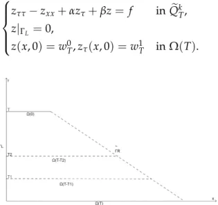
In order to define the transposition solution of (1.2), we introduce the following backward

Figure 1.1: The graph of (1.2) system with zero terminal value.











wtt−wxx−αwt+βw= f inQ^k_T, w|_ΓL =0,

w(x,T) =0,w_t(x,T) =0 inΩ(T).

(1.3)

Set H_L¹(_Ω(t)) = {w ∈ H¹(_Ω(t)) | the trace ofwvanish at x=0}, ∀t ≥ 0. Assume that F is a functional space and F⁰ is its dual space. Leth·,·i_F,F⁰ denote the dual product between them.

Proposition 1.1. For any f ∈ L²(Q^k_T), (1.3)admits a unique weak solution w∈ L²(0,T;H¹_L(_Ω(t)))^\H¹(0,T;L²(_Ω(t))).

Definition 1.2. Let T > 0. u ∈ L²(0,T;L²(_Ω(t)))^TH¹(0,T;H⁻¹(_Ω(t))) is called a trans- position solution of (1.2), if for any (u⁰,u¹) ∈ L²(_Ω(0))×H⁻¹(_Ω(0)), f₁ ∈ L²(_ΓL) and

f₂,f₃∈ L²(_ΓR),usatisfies the following equality Z

Q^k_T

f udxdt=hw(₀)_,u¹i_H1

L(_Ω(₀)),H⁻¹(_Ω(₀))−

Z

Ω(0)

[u⁰w_t(₀)−αu⁰w(₀)]dx +

Z

ΓL

f₁w_xds+

Z

ΓR

w f₃+ f₂(−kw_t−w_x+kαw)

√1+k²

ds, ∀f ∈ L²(Q^k_T), (1.4)

wherewis the solution of (1.3).

The main result of this paper is stated as follows.

Theorem 1.3. For any given(u⁰,u¹)∈ L²(_Ω(0))×H⁻¹(_Ω(0)), f₁∈ L²(_ΓL)and f2,f3 ∈ L²(_ΓR), (1.2)admits a unique solution

u∈ L²(0,T;L²(_Ω(t)))^\H¹(0,T;H⁻¹(_Ω(t))) in the sense of transposition.

In addition, we study the energy for the homogeneous system of (1.2):











u_tt−u_xx+αu_t+βu=0 in Q^k_T, u|_ΓL =0,u|_ΓR =0,^∂u_∂l|_ΓR =0,

u(x, 0) =u⁰,u_t(x, 0) =u¹ inΩ(0),

(1.5)

where(u⁰,u¹)is given in (1.2).

Concerning wave equations in domains with variable boundaries, the work on stability and stabilization has been addressed much less in the literature. For the case of time-like domains, we mention [3,11], which provided some first-order polynomial decay results using the multiplier method. As we know, the multiplier method is an efficient way to get a poly- nomial decay estimate (see e.g. [10]), but it requires that the coefficients of wave equations satisfy certain constraints (e.g. for (1.5), α² = 4β needed) and depending on the multiplier method, it is hard for us to obtain a better decay estimate. For the sake of getting the desired exponential decay of the energy for (1.5), we borrow an idea introduced in [9]. The difference is the use of an auxiliary functional ρ which will be provided in Section 4. We focus on the case of α,β > 0 below. On the one hand, when α = 0 and β = 0, it is easy to check the energyE(t) = ¹₂R

Ω(t)[u²_t(x,t) +u²_x(x,t)]dxfor (1.5) is conserved. On the other hand, if either of α,β > 0 is not true, we have not been able to get the energy estimate for such a problem (we shall provide a further interpretation in Remark4.1, Section 4).

Define an energy functional:

E(u;t) = ¹ 2

Z

Ω(t)

u²_t(x,t) +u²_x(x,t) +βu²(x,t)dx.

The energy estimate for (1.5) is as follows.

Theorem 1.4. There exist constantsε₁>0and c₁ >0(only depend onαorβ),such that the energy functional of(_1.5)satisfies

E(u;t)≤ ²

1−c₁εexp

− ^εt 1+c₁ε

E(u; 0), ∀0<ε ≤ε₁, ∀t≥0. (1.6) Throughout this paper, we letCrepresent a positive constant which may be different from one line to another. For simplicity of presentation, in what follows we omit the variables of functions sometimes when they are clear in the text.

Remark 1.5. We wish to present an interpretation for the form of (1.4). Without loss of gen- erality, we may assume that functions are sufficiently smooth. Otherwise, we can use the smoothing technique. Ifuis a solution of (1.2), multiplying the first equation of (1.2) bywand integrating the both sides of the equation onQ^k_T, we have

Z

Q^k_T

(u_tt−u_xx+αu_t+βu)wdxdt=0, that is,

Z

Q^k_T

[(u_tw−uw_t+αuw)_t−(u_xw−uw_x)_x+u(w_tt−w_xx−αw_t+βw)]dxdt=0.

Using Green’s formula, we obtain Z

∂Q^k_T

[(u_tw−uw_t+αuw)n_t−(u_xw−uw_x)n_x]ds+

Z

Q^k_Tu(w_tt−w_xx−αw_t+βw)dxdt=0, where ds is the length of an infinitesimal on boundary ∂Q^k_T. Notice that the unit exterior normaln(p) = (nx(p),nt(p))^>= (0, 1)^>,(0,−1)^>,(−1, 0)^>and ^{√ 1}

1+k²,^√−k

1+k²

>

when p lies in

Ω(T),Ω(0),ΓL andΓR, respectively. Substituting them into the above equation, we get Z

Ω(T)

(utw−uwt+αuw)(x,T)dx−

Z

Ω(0)

(utw−uwt+αuw)(x, 0)dx +

Z

ΓL

(uxw−uwx)ds+

Z

ΓR

−w(ku_t+u_x)

√

1+k² +u(kw_t+w_x−kαw)

√ 1+k²

ds +

Z

Q^k_Tu(w_tt−w_xx−αw_t+βw)dxdt=0,

where we follow the expression (u+w)(x,T) =u(x,T) +w(x,T).

Further, ifw is a solution of (1.3), due to the approximation theory of smooth functions, we arrive at

hw(0),u¹i_H1

L(_Ω(0)),H⁻¹(_Ω(0))−

Z

Ω(0)

[u⁰w_t(0)−αu⁰w(0)]dx +

Z

ΓL

uwxds+

Z

ΓR

w(kut+ux)

√

1+k² +u(−kwt−wx+kαw)

√ 1+k²

ds=

Z

Q^k_Tu f dxdt.

Remark 1.6. We would like to show some connections between our results and the existing results. As we know, the definite conditions of the string equation defined inR+are the initial displacement and the initial velocity. If we letk→+∞, then in (1.2), the moving boundaryΓR

goes to thex+axis and the directionl= ^√1

1+k²,^√k

1+k²

→(0, 1). At that time,u|_ΓR becomes a displacement and ^∂u_∂l|_ΓR becomes a velocity. On the other hand, if we let k→_{1, then ΓR turns} into a characteristic line of the string equation and l → ^√1

2,^√1

2

, which is the characteristic direction. According to the compatibility principle, we infer that the boundary conditions in (1.2) become the boundary conditions of the case k=1.

The rest of this paper is organized as follows. In Section 2, we prove Proposition 1.1. In Section 3, we prove Theorem1.3. In Section 4, we deduce the energy estimate. Section 5 offers an appendix which is a supplement to the proof of Proposition2.1in Section 2.

2 The wellposedness of (1.3)

In this section, we start to prove Proposition 1.1. More generally, we consider systems with any given terminal value.

First, we consider the following pure wave system:











wtt−wxx= f inQ^k_T, w|_ΓL =_0,

w(x,T) =w⁰_T,w_t(x,T) =w¹_T inΩ(T).

(2.1)

Proposition 2.1. For any given(w⁰_T,w¹_T)∈ H¹_L(_Ω(T))×L²(_Ω(T))and f ∈ L²(Q^k_T), (2.1)admits a unique solution w ∈L²(0,T;H¹_L(_Ω(t)))^TH¹(0,T;L²(_Ω(t))).

We postpone the proof of Proposition2.1until the appendix for standing out the main part of this paper.

Next consider the system as follows.











w_tt−w_xx−αw_t+βw= f inQ^k_T, w|_ΓL =0,

w(x,T) =w⁰_T,w_t(x,T) =w¹_T inΩ(T).

(2.2)

Proposition 2.2. For any given (w⁰_T,w¹_T) ∈ H¹_L(_Ω(T))×L²(_Ω(T))and f ∈ L²(Q^k_T), (2.2)admits a unique solution w∈ L²(0,T;H_L¹(_Ω(t)))^TH¹(0,T;L²(_Ω(t))).

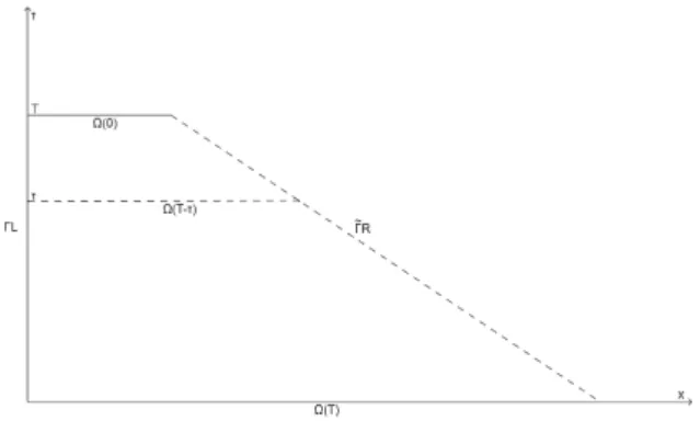
Our idea for the proof of Proposition2.2is to transform the backward system into an equiva- lent forward system. Then we use the contraction mapping principle and an energy method to finish the proof. As a preliminary, some notations are given ahead. Writeeα_k(τ) =1+k(T−τ) for 0≤τ ≤ T. We let Qe^k_T stand for a non-cylindrical domain inR² : Qe^k_T ={(x,τ)∈ _R² |0<

x < _eα_k(τ), 0 < τ < T}. PutΓL = {(0,τ)∈ _R² | τ ∈ [0,T]}andeΓR = {(_eα_k(τ),τ) ∈ _R² |τ ∈ [0,T]}(see Figure2.1).

Proof. Step 1. If we take a time transformationτ= T−tand letz(x,τ) =w(x,T−τ), then we see that the wellposedness of (2.2) is equivalent to the wellposedness of the following system:











zττ−z_xx+αzτ+βz = f inQe^k_T, z|_ΓL =0,

z(x, 0) =w⁰_T,z_τ(x, 0) =w¹_T inΩ(T).

(2.3)

Figure 2.1: The graph of (2.3)

Let 0<T₁ <T and putQe₀^T1 ={(x,τ)∈_R² |0<x <1+k(T−τ), 0<τ< T₁}. Consider the following system with respect to (2.3) in Qe^T₀¹:











zττ−zxx+αξ_τ+βξ= f inQe₀^T1, z(0,τ) =0 on(0,T₁), z(x, 0) =w⁰_T,zτ(x, 0) =w¹_T inΩ(T).

(2.4)

Set X = L²(0,T₁;H_L¹(_Ω(T−τ)))^TH¹(0,T₁;L²(_Ω(T−τ))), where Ω(T−τ) = {(x,τ) ∈ R²|0 < x < 1+k(T−τ)} and put kzk²_X = R

Qe^T₀¹[z²_τ(x,τ) +z²_x(x,τ)]dxdτ, ∀z ∈ X. X is a Banach space with the norm k · k_X which can be found in [1]. Define a mapping F : ξ 7→ z,

∀ξ ∈ X, wherez is the solution of (2.4). By Proposition2.1,F is well defined. Next we prove Fis a contraction mapping onX. Letz1 = _F(ξ₁)_andz2 =_F(ξ₂)_, ∀ξ₁,ξ₂ ∈ X. Putξ =ξ₁−ξ₂ andz= z₁−z₂. From the linearity of (2.4), we know thatz andξ satisfy











zττ−z_xx+αξ_τ+βξ =0 in Qe^T₀¹, z(0,τ) =0 on (0,T₁), z(x, 0) =0,z_τ(x, 0) =0 in Ω(T).

(2.5)

Multiplying both sides of the first equation of (2.5) byz_τ, we get (z_ττ−z_xx)z_τ = (−αξ_τ−βξ)z_τ. Furthermore,

1

2(z²_τ+z²_x)_τ−(z_τz_x)_x= (−αξ_τ−βξ)z_τ.

For any τ₁ ∈ (0,T₁], integrating the above equality on(0,τ₁)×_Ω(T−τ)and observing that n(p) = (nx(p),nτ(p))^>= ^{√ 1}

1+k²,^{√ k}

1+k²

>

, ∀p∈eΓR, we have Z

Ω(T−τ₁)

1 2

z²_τ(_x,τ₁) +_z²_x(_x,τ₁)_dx+

Z

eΓR

1

2(_z²_τ+_z²_x)√ ^k

1+k² −√ ¹

1+k²zτzx

ds

=

Z _τ1

0

Z

Ω(T−τ)

(−αξ_τ−βξ)z_τdxdτ.

Due to k>_{1, we get}

Z

Ω(T−τ1)

1 2

z²_τ(x,τ₁) +z²_x(x,τ₁)dx

≤

Z _τ1

0

Z

Ω(T−τ)

(−αξ_τ−βξ)zτdxdτ

≤

Z

Qe^T₀¹

(α²ξ²_τ+β²ξ²)dxdτ+

Z _τ1

0

Z

Ω(T−τ)

1 2

z²_τ(x,τ) +z²_x(x,τ)dxdτ.

Using Gronwall’s inequality, we arrive at Z

Ω(T−τ₁)

1 2

z²_τ(x,τ₁) +z²_x(x,τ₁)dx≤e^τ1 Z

Qe^T₀¹

(α²ξ²_τ+β²ξ²)dxdτ. (2.6) We start to estimate R

Qe₀^T1 ξ²dxdτ. Since ξ ∈ X, ξ(0,τ) = 0, a.e. τ ∈ (0,T₁) and ξ(x,τ) = Rx

0 ξ_y(y,τ)dy. Using Hölder’s inequality, we have ξ²(x,τ) =

_{Z x}

0 ξ_y(y,τ)dy 2

≤x Z _x

0 ξ²_y(y,τ)dy.

Moreover, 0≤x ≤₁+k(T−τ)_,∀τ∈[_0,T₁]_{, so}

Z _1+k(T−τ)

0 ξ²(x,τ)dx≤

Z _1+k(T−τ)

0 x

Z _x

0 ξ²_y(y,τ)dydx

≤

Z _1+k(T−τ)

0

[₁+k(T−τ)]

Z _1+k(T−τ)

0

ξ²_y(y,τ)dydx

≤[1+k(T−τ)]²

Z _1+k(T−τ)

0 ξ²_y(y,τ)dy.

Integrating the above inequality on (0,T₁), one has Z

Qe^T₀¹ ξ²(x,τ)dxdτ≤(1+kT)²

Z

Qe₀^T1ξ²_x(x,τ)dxdτ. (2.7) Using (2.7) in (2.6), one gets

Z

Ω(T−τ1)

1 2

z²_τ(x,τ₁) +z²_x(x,τ₁)dx≤e^τ1 Z

Qe^T₀¹

h

α²ξ²_τ+β²(1+kT)²ξ²_x i

dxdτ.

Since the above inequality holds for anyτ₁ ∈(0,T₁], integrating it on(0,T₁), we obtain Z

Qe^T₀¹

1 2

z²_τ(x,τ) +z²_x(x,τ)dxdτ≤ T₁e^T1 Z

Qe^T₀¹

h

α²ξ²_τ+β²(1+kT)²ξ²_x i

dxdτ

≤ T₁e^T1max{α²,β²(1+kT)²}

Z

Qe₀^T1

(ξ²_τ+ξ²_x)dxdτ.

This implies that

kzk_X ≤^h2T₁e^T1max{α²,β²(1+kT)²}ⁱ

1 2 kξk_X.

We can chooseT₁ to be small such thatkzk_X ≤ ¹₂kξk_X holds, i.e.,kF(ξ₁)−F(ξ₂)k_X ≤ ¹₂kξ₁− ξ₂k_X. For this T₁, F is a contraction mapping on X. According to the contraction mapping principle, we know that F has a fixed point in X which is a solution of (2.3) in Qe^T₀¹. Let T0 = 0 and T₁ = T₁. For any T_i(i ≥ 0,i ∈ _Z), we put Qe^T_Tⁱ⁺¹

i = {(x,τ) ∈ _R² | 0 < x <

1+k(T−τ),T_i <τ<T_i+1}andX_i = L²(T_i,T_i+1;H¹_L(_Ω(T−τ)))^TH¹(T_i,T_i+1;L²(_Ω(T−τ))). Going through the same process we used in Qe^T₀¹ for Qe^T_Tⁱ_i⁺¹, we can get kzk_Xi ≤ 2(T_i+1− T_i)e^(Ti+1−Ti)max{α²,β²(1+k(T−T_i))²}¹²kξk_Xi. Let T_i+1−T_i ≤ T₁, then we have

2(T_i+1− T_i)e^(Ti+1−Ti)max{α²,β²(1+k(T−T_i))²}¹² ≤ 2T₁e^T1max{α²,β²(1+kT)²}¹², which implies that Fis a contraction mapping on everyX_i. Continuing this process untilT_i+1 ≥T for some i, we deduce that (2.3) admits a solution inQe^k_T.

Step 2. We shall use an energy method for proving the uniqueness of the solution. Multiplying both sides of the first equation of (2.3) byz_τ, we have

(z_ττ−z_xx+αz_τ+βz)z_τ = f z_τ. Further,

1

2(z²_τ+z²_x+βz²)_τ−(z_xz_τ)_x+αz²_τ = f z_τ.

For any T₁in (0,T], integrating the above equality onQe₀^T1 and using the boundary condition again, we get

Z

Ω(T−T₁)

1 2

z²_τ(x,T₁) +z²_x(x,T₁) +βz²(x,T₁)dx

≤

Z _T1

0

Z

Ω(T−τ)

(f zτ−αz²_τ)dxdτ+

Z

Ω(T)

1 2

"

(w¹_T)²+ ∂w⁰_T

∂x 2

+β(w⁰_T)²

# dx

≤

Z _T1

0

Z

Ω(T−τ)

1 2δf²+

δ 2−α

z²_τ

dxdτ+

Z

Ω(T)

1 2

"

(w¹_T)²+ ∂w⁰_T

∂x 2

+β(w⁰_T)²

# dx.

Ifα>0, we can choose ₂^δ <α; ifα=0, we use Gronwall’s inequality again. Hence Z

Ω(T−T1)

1 2

z²_τ(x,T₁) +z²_x(x,T₁) +βz²(x,T₁)dx

≤C(T)

"

Z

Qe^k_T f²dxdτ+

Z

Ω(T)

1 2

"

(w¹_T)²+ ∂w⁰_T

∂x 2

+β(w⁰_T)²

# dx

# .

(2.8)

Because (2.8) holds for every T₁ ∈ [_0,T], it is shown that the solution of (2.3) is unique. The conclusion of Proposition2.2follows from the equivalence of wellposedness between (2.2) and (2.3).

In Proposition2.2, letting(w⁰_T,w¹_T) = (_{0, 0}), we have Proposition1.1.

3 The proof of Theorem 1.3

This section is devoted to establishing a hidden regularity result for (1.3) by the multiplier technique and confirming the conclusion of Theorem 1.3. We divide our proof in three steps.

Proof. Step 1. Define a functionalF:∀f ∈ L²(Q^k_T), F(f) =hw(0),u¹i_H1

L(_Ω(0)),H⁻¹(_Ω(0))−

Z

Ω(0)

(u⁰wt(0)−αu⁰w(0))dx Z

ΓL

f₁w_xds+

Z

ΓR

w f₃+ f₂(−kw_t−w_x+kαw)

√1+k²

ds,

(3.1)

where wis the solution of (1.3) with f. In (3.1),u⁰,u¹, f₁, f₂and f₃ are known. It is clear that Fis a linear functional. Next, we are going to prove it is bounded.

Step 2. We multiply both sides of the first equation of (1.3) by w_t and integrate it on Q^k_T. Observing thatn(p) = (n_x(p),n_t(p))^>= (^√1

1+k²,^√−k

1+k²)^>,∀p∈_ΓR, we have Z

Q^k_T f w_tdxdt=

Z

Q^k_T(w_tt−w_xx−αw_t+βw)w_tdx

=

Z

Q^k_T

1

2(w²_t +w²_x+βw²)_t−(w_tw_x)_x−αw²_t

dxdt

= −E(0) +

Z

ΓR

1

2(w²_t +w²_x+βw²) −k

√

1+k² −(wtwx)√ ¹ 1+k²

ds

−α Z

Q^k_Tw²_tdxdt,

(3.2)

where E(t) =R

Ω(t) 1 2

w²_t(x,t) +w²_x(x,t) +βw²(x,t)dx.

From (2.8), when(w⁰_T,w¹_T) = (0, 0), we know E(t)≤C(T)

Z

Q^k_T f²dxdt, ∀t ∈[0,T]. (3.3) Step 3. Multiplying both sides of the first equation of (1.3) by w_x and integrating it on Q^k_T, we get

Z

Q^k_T f w_xdxdt=

Z

Q^k_T

(w_tt−w_xx−αw_t+βw)w_xdx

=

Z

Q^k_T

(wtwx)_t− ¹

2(w²_t +w²_x−βw²)_x−αwtwx

dxdt

= −

Z

Ω(0)w_t(x, 0)w_x(x, 0)dx+

Z

ΓL

1 2w²_xds +

Z

ΓR

w_tw_x −k

√

1+k² −¹

2(w²_t +w²_x−βw²)√ ¹ 1+k²

ds−α

Z

Q^k_Tw_tw_xdxdt.

(3.4)

(3.4)−k×(3.2), yields Z

Q^k_T

(f w_x−k f w_t)dxdt=−

Z

Ω(0)w_t(x, 0)w_x(x, 0)dx+

Z

ΓL

1 2w²_xds +

Z

ΓR

−¹

2(w²_t +w²_x−βw²)√ ¹

1+k² + ¹

2(w²_t +w²_x+βw²) ^k

2

√1+k²

ds +

Z

Q^k_T

(−αwtwx+kαw²_t)dxdt+kE(0).

Rearranging the above equality, we obtain Z

ΓL

1

2w²_xds+

Z

ΓR

(k²−1) 2√

1+k²(w²_t +w²_x) + (k²+1)β 2√

1+k²w²

ds

=

Z

Q^k_T

f(w_x−kw_t) +α(w_tw_x−kw²_t)dxdt+

Z

Ω(0)w_t(x, 0)w_x(x, 0)dx−kE(0)

≤ C(α,β,k,T)

Z

Q^k_T f²dxdt,

(3.5)

where the last inequality in (3.5) is derived using (3.3). From (3.5), it follows that wx|_ΓL ∈ L²(_ΓL),w|_ΓR,w_t|_ΓR andw_x|_ΓR ∈ L²(_ΓR). We shall make the assumptions:(u⁰,u¹)∈ L²(_Ω(0))× H⁻¹(_Ω(0)),f₁ ∈L²(_ΓL),f₂ ∈ L²(_ΓR)and f₃ ∈L²(_ΓR). The definition forF(f)in (3.1), together with (3.5), indicates that there exists a positive constantC (only depending onα,β,k,T) such that

|F(f)| ≤C(_α,β,k,T)^hk(u⁰,u¹)k_L2(_Ω(0))×H⁻¹(_Ω(0))+kf₁k_L2(_ΓL)+kf₂k_L2(_ΓR)+kf₃k_L2(_ΓR)

ikfk_L2(Q^k_T). According to the Riesz’s theorem, one can find a uniqueu∈ L²(0,T;L²(_Ω(t)))such that (1.4) holds. We claim that (1.2) has a unique solutionu∈ L²(0,T;L²(_Ω(t)))in the sense of transpo- sition. Without loss of generality, letg∈C₀^∞(_0,T;H₀¹(_Ω(t)))and replace f withg_tat the right end of the first equation in (1.3). In the same manner we can get ^∂u_∂t ∈ L²(0,T;H⁻¹(_Ω(t))).

4 The proof of Theorem 1.4

In this section, we prove Theorem1.4 for the system (1.5) in Section 1.

Noticing thatu|_ΓR =0 and ^∂u_∂l|_ΓR =0 in (1.5), we can deduce that ux|_ΓR =ut|_ΓR =0.

Thus the boundary conditions in (1.5) are equivalent to

u|_ΓL =0, u|_ΓR =ux|_ΓR = ut|_ΓR =0. (4.1) Inspired by [9], we introduce an auxiliary functional. For anyε>0, let

E_ε(u;t) =E(u;t) +ερ(u;t)_, ∀t≥0, where

ρ(u;t) =

Z _αk(t)

0 ut(x,t)u(x,t)dx.

Proof. First, suppose that the initial value(u⁰,u¹)and the solutionuare sufficiently smooth.

On account of

|ρ(u;t)| ≤

Z _αk(t)

0

|utu|dx≤ ¹ 2

Z _αk(t)

0

(¹

βu²_t +βu²+u²_x)dx, whenβ≥1, putc₁ =1; whenβ<1, put c₁ = ¹

β. Hence,

ε⁻¹|E_ε(u;t)−E(u;t)|=|ρ(u;t)| ≤c₁E(u;t)_{. (4.2)}

Using the first equation in (1.5), we have E_ε⁰(u;t) =E⁰(u;t) +ερ

0(u;t)

=

Z _αk(t)

0

(u_tu_tt+u_xu_xt+βuu_t)dx+ε Z _αk(t)

0

(u_ttu+u²_t)dx

=

Z _αk(t)

0

u_t(u_xx−αu_t−βu) +u_xu_xt+βuu_t dx +ε

Z _αk(t)

0

(uxx−αut−βu)u+u²_t dx

=

Z _αk(t) 0

(u_tu_x)_x−αu²_t dx +ε

Z _αk(_t) 0

(u_xu)_x−u²_x−αu_tu−βu²+u²_t dx, where E⁰_ε(u;t)represents the derivative ofE_ε(u;t)with respect to time.

Using (4.1), we arrive at E⁰_ε(u;t) =−α

Z _αk(t)

0 u²_tdx+ε Z _αk(t)

0

(−u²_x−αu_tu−βu²+u²_t)dx.

Furthermore, ε

Z _αk(t)

0

(−u²_x−αu_tu−βu²+u²_t)dx

≤ε Z _αk(t)

0

−¹ 2u²_x+

β 2u²+ ^α

2

2βu²_t

−βu²+u²_t

dx

=ε Z _αk(t)

0

−¹

2 u²_x+βu²+u²_t +

3 2 + ^α

2

2β

u²_t

dx

=−εE(u;t) +ε 3

2+ ^α

2

2β _{Z α}

k(t) 0 u²_tdx.

Lettingε≤ ^α

3

2+_2β^α2 =ε0, we have

E⁰_ε(u;t)≤ −εE(u;t). On the other hand, whenε< _c¹

1, (4.2) implies that

(1−c₁ε)E(u;t)≤ Eε(u;t)≤(1+c₁ε)E(u;t), ∀t≥0.

So

E⁰_ε(u;t)≤ −εE(u;t)≤ − ^ε

1+c₁εEε(u;t). (4.3) Setε₁=min₁

c1,ε₀ . Using (4.2) combined with (4.3), we get (1−c₁ε)E(u;t)≤Eε(u;t)≤exp

− ^εt 1+c₁ε

Eε(u; 0)

≤exp

− ^εt 1+c₁ε

(1+c₁ε)E(u; 0),

∀0< ε≤ε₁, ∀t ≥0.

It means that

E(u;t)≤exp

− ^εt 1+c₁ε

1+c₁ε

1−c₁εE(u; 0)

≤ ² 1−c₁εexp

− ^εt 1+c₁ε

E(u; 0), ∀t≥0.

(4.4)

Finally, using the approximation theory of smooth functions in(4.4), we obtain Theorem1.4.

Remark 4.1. From the process of the proof of Theorem1.4, we can see that ifα≤0, the energy of (1.5) does not decrease; if β = 0, we are not able to get the desired decay estimate in the same manner (because the Poincaré inequality does not hold for some uniform constant in such an increasing domain).

Remark 4.2. In the case of 0 < _k ≤ 1, by [5], we have that the wave equation is well-posed with two Dirichlet boundary conditions. We can also put a damping αut (α > 0) and a compensation βu (β > 0) into the homogeneous system to consider the energy estimate.

Although there will be some extra terms coming from boundary, we can deal with them as well depending on the method mentioned above, and then get the exponential decay results.

Nevertheless, if the moving boundaries are general, things may be complicated and it may be not easy for us to deal with those boundary terms and get the desired energy estimate based on the method above.

5 Appendix. The proof of Proposition 2.1

We follow the notations in Section 2.

Proof. Taking a time transformation τ = T−t and letting z(x,τ) = w(x,T−τ), we change (2.1) to the following system ofz:











zττ−z_xx= f inQe^k_T, z|_ΓL =0,

z(x, 0) =w⁰_T,z_τ(x, 0) =w¹_T inΩ(T).

(5.1)

We will denote by Qe^k_T the closure of Qe^k_T and by D(Qe^k_T) the space of infinitely differentiable functions defined onQe^k_T. Let (D(Qe^k_T))² be the quadratic space ofD(Qe^k_T)andH = (L²(Qe^k_T))².

∀Y,W ∈ H, withY = (y₁,y₂)^> andW = (w₁,w₂)^>, an inner product inH is defined to be (Y,W)_H=

Z

Qe^k_T

y₁(x,t)w₁(x,t) +y₂(x,t)w₂(x,t)dxdt.

We use the symbolh·,·i_R2 to denote the scalar product inR². The notation | · |_R2 means the canonical norm induced byh·,·i_R2. Define an operator A:

D(A) ={W ∈ H | AW ∈ H}, AW =

∂w1

∂t − ^∂w_∂x²

∂w2

∂t − ^∂w_∂x¹

!

, ∀W = (w₁,w₂)^> ∈D(A).