Asymptotic behavior of solutions of a Fisher equation with free boundaries and nonlocal term
Jingjing Cai
B, Yuan Chai, Lizhen Li and Quanjun Wu
School of Mathematics and Physics, Shanghai University of Electric Power, Pingliang Road 2103, Shanghai 200090, China
Received 22 December 2018, appeared 30 October 2019 Communicated by Eduardo Liz
Abstract. We study the asymptotic behavior of solutions of a Fisher equation with free boundaries and the nonlocal term (an integral convolution in space). This problem can model the spreading of a biological or chemical species, where free boundaries represent the spreading fronts of the species. We give a dichotomy result, that is, the solution either converges to 1 locally uniformly inR, or to 0 uniformly in the occupying domain. Moreover, we give the sharp threshold when the initial data u0 =σφ, that is, there existsσ∗>0 such that spreading happens whenσ>σ∗, and vanishing happens whenσ≤σ∗.
Keywords: asymptotic behavior of solutions, free boundary problem, Fisher equation, nonlocal.
2010 Mathematics Subject Classification: 35K20, 35K55, 35B40, 35R35.
1 Introduction
Consider the following free boundary problem with nonlocal term
ut =uxx+ (1−u)
Z
Rk(x−y)u(t,y)dy, g(t)<x <h(t), t>0, u(t,x) =0, x∈R\(g(t),h(t)), t>0, g0(t) =−µux(t,g(t)), t >0,
h0(t) =−µux(t,h(t)), t >0,
−g(0) =h(0) =h0, u(0,x) =u0(x), −h0≤ x≤h0,
(1.1)
where x = g(t)andx = h(t) are moving boundaries to be determined together withu(t,x), µ>0 is a constant, h0>0. We use the standard hypotheses on kernel k(·)as follows:
k ∈C1(R)is nonnegative, symmetric and Z
Rk(x−y)dy= 1 for anyx∈R. (1.2)
BCorresponding author. Email: cjjing1983@163.com
The initial functionu0belongs toX(h0)for someh0 >0, where
X(h0):= nφ∈ C2([−h0,h0]):φ(−h0) =φ(h0) =0, φ(x)≥ (6≡)0 in(−h0,h0)o. (1.3) Recently, Problem (1.1) with Fisher–KPP nonlinearity, i.e.,ut =uxx+u(1−u)was studied by [9,10], etc. They used this model to describe the spreading of a new or invasion species, with the free boundariesh(t)andg(t)representing the expanding fronts of the species whose den- sity is represented byu(t,x). They obtained a spreading-vanishing dichotomy result. More- over, [10] also studied the bistable nonlinearity and obtained a trichotomy result. Later, [2–4]
also considered Fisher–KPP equation with other free boundary conditions. [11,13,14] also studied the corresponding problem of (1.1) with Fisher–KPP nonlinearity in high dimensional spaces (without nonlocal term).
It is known that some species are distributed in space randomly. They typically inter- act with physical environment and other individuals in their spatial neighborhood, so some species u at a point x and time t usually depend on u in the neighborhood of the point x.
And they even depend onuin the whole region. Therefore, we added the nonlocal term into the equation, i.e., R
Rk(x−y)u(t,y)dy, instead of u to model the growth of the species. The reason why this is a global term is that the population are moving, and then, the growth of the species is related to the population in a neighborhood of the original position. Hence, the growth rate of the species can be represented as a spatial weighted average. For the above reasons, we added the nonlocal term into the equation. Such nonlocal interactions are also used in epidemic reaction-diffusion models, such as [7] studied the following system
(ut =d∆u−au+R
Ωk(x,y)v(t,y)dy, t >0, x∈Ω,
vt=−bv+G(u), t >0, x∈Ω (1.4)
with conditionsβ(x)∂u∂n+α(x)u=0 and β(x)∂v∂n+α(x)v=0 fort >0 andx∈ ∂Ω. k(x,y)>0 is symmetric and R
Rk(x,y)dy = 1. They studied the globally asymptotic stability of the trivial solution and the existence of the nontrivial equilibrium which is globally asymptotically stable. There are many other papers (cf. [16,18,19] and so on) studied nonlocal problem of reaction-diffusion systems in bounded/unbounded domain. Recently, some authors introduce free boundaries to such nonlocal problems, [15] studied (1.4) (with k(x,y) is replaced by k(x−y)) forx∈ [g(t),h(t)]with free boundariesg(t)andh(t)satisfyingg0(t) =−ux(t,g(t)), h0(t) = −ux(t,h(t)), they obtained some sufficient conditions for spreading and vanishing, when spreading happens, they also give the estimates of the asymptotic spreading speed. [6]
also considered the nonlocal SIS epidemic model with free boundaries and obtained some sufficient conditions for spreading (limt→∞ku(t,·)kC([g(t),h(t)]) >0) and vanishing.
In this paper, we will introduce the nonlocal term to the free boundary problem of the Fisher equation, i.e., the problem (1.1). We see that this problem indicates that the whole class exhibit themselves on the whole region R. The individuals occupy the initial region [−h0,h0]and invade further into the new environment from two ends of the initial region. The spreading fronts spread at a speed that is proportional to the population gradient at the fronts, that is, they satisfy the Stefan conditionsh0(t) =−µux(t,h(t))andg0(t) =−µux(t,g(t)). Since the individuals are moving, the nonlocal term in (1.1) means that the individuals at location x can contact with susceptible individuals in the neighborhood of location x or the whole class, this gives rise to the nonlocal effect. We will give more explicit asymptotic behavior of solutions and consider the effect of the nonlocal term on the spreading of the solution. We first give some sufficient conditions for spreading (limt→∞g(t) =−∞, limt→∞h(t) = +∞and
the solution u converges to 1) and vanishing (0 < limt→∞h(t)−limt→∞g(t) < 2`∗ and the solution uconverges to 0, where the definition of `∗ > 0 is given in Section 2), then obtain a spreading-vanishing dichotomy. We finally give the sharp threshold result: when the initial data u0 = σφ, there is critical value σ∗ > 0, when σ ≤ σ∗, vanishing happens; whenσ > σ∗, spreading happens.
We first give the existence of the solution of the problem (1.1) and some basic properties of g(t)and h(t). It follows from the arguments in [9] (with obvious modifications) that the problem (1.1) has a unique solution
(u,g,h)∈C1+γ2,1+γ(D)×C1+γ/2([0,+∞))×C1+γ/2([0,+∞))
for any γ ∈ (0, 1), where D := {(t,x) ∈ R2 : x ∈ [g(t),h(t)],t ∈ (0,+∞)}. By the strong comparison principle and the Hopf lemma, we also haveh0(t)>0 andg0(t)<0 for all t>0.
Hence
h∞ := lim
t→∞h(t)∈(0,+∞] and g∞ := lim
t→∞g(t)∈[−∞, 0) exist. Moreover, as in the proof of [10, Lemma 2.8] one can show that
−2h0< g(t) +h(t)<2h0 for all t>0. (1.5) We conclude from this inequality that I∞ := (g∞,h∞)is eitherRor a finite interval.
The main purpose of this paper is to study the asymptotic behavior of bounded solutions of (1.1).
Theorem 1.1. Assume that(u,g,h)is a time-global solution of (1.1). Then either (i) spreading: (g∞,h∞) =Rand
tlim→∞u(t,x) =1locally uniformly inR, or
(ii) vanishing: (g∞,h∞)is a finite interval with length no bigger than2`∗, and limt→∞ max
g(t)≤x≤h(t)u(t,x) =0, where the definition of`∗ is given in Proposition2.1.
Moreover, if u0= σφwithφ∈ X(h0), then there existsσ∗ =σ∗(h0,φ)≥0such that vanishing happens whenσ≤σ∗, and spreading happens whenσ>σ∗.
In Section 2, we show some preliminary results including the eigenvalue problem and comparison principle theorem. In Section 3, we first give sufficient conditions of spreading and vanishing, then prove the main theorem. In Section 4, we give the Appendix to prove incomplete or unproved statements of this paper.
2 Some preliminary results
In this section, we first consider the eigenvalue problem and discuss the properties of the principal eigenvalue, which plays an important role in studying spreading and vanishing. We then give the comparison principle theorems. Finally, we consider the convergence of the solutions of elliptic equations, which is used to prove spreading.
2.1 Eigenvalue problem
We consider the following eigenvalue problem
φxx+
Z `
−`k(x−y)φ(y)dy+λφ=0, x∈(−`,`), φ(−`) =φ(`) =0,
(2.1) for any` > 0. The principal eigenvalue of (2.1) is the smallest eigenvalue, which is the only eigenvalue admitting a positive eigenfunction except forx = ±`. It is well-known that (2.1) has a unique principal eigenvalue (cf. LemmaA.2in Appendix), denoted byλ1(`), and there is a positive eigenfunctionφ1 withkφ1kL2([−`,`])=1 corresponding toλ1(`), andλ1(`)can be characterized by
λ1(`) = inf
φ∈C0([−`,`]),φ6≡0
R`
−`(φ0(x))2dx−R`
−`
R`
−`k(x−y)φ(x)φ(y)dxdy R`
−`φ2(x)dx
!
, (2.2) whereφ∈C0([−`,`])means thatφ∈C([−`,`])withφ(±`) =0. Moreover, for any`1,`2 >0, Corollary 2.3 in [5] says thatλ1(`1) > λ1(`2) when`1 < `2. (The proof of this conclusion is given in Appendix).
Proposition 2.1. There is a`∗ ≥ π/2 such thatλ1(`) > 0when ` < `∗,λ1(`) = 0 when ` = `∗ andλ1(`)<0when` > `∗.
Proof. Due to Z
R
Z
Rk(x−y)φ(x)φ(y)dxdy
≤
Z
R
Z
Rk(x−y)φ
2(x) +φ2(y)
2 dxdy
= 1 2
Z
Rφ2(y)dy Z
Rk(x−y)dx+1 2
Z
Rφ2(x)dx Z
Rk(x−y)dy
=
Z `
−`φ2(x)dx (note that Z
Rk(x−y)dy=1),
(2.3)
we have
λ1(`)≥ inf
φ∈C0,φ6≡0
R`
−`(φ0(x))2dx R`
−`φ2(x)dx
− sup
φ∈C0,φ6≡0
R`
−`
R`
−`k(x−y)φ(x)φ(y)dxdy R`
−`φ2(x)dx
≥ π2 4`2 −1.
(2.4)
Here we have used the well known result:
R`
−`(φ0(x))2dx R`
−`φ2(x)dx attains its minimum atφ(x) =cos(πx2`). Hence, it follows from (2.4) that
λ1(`)>0 when ` < π
2. On the other hand, takingφ(x) =cos(πx2`)in (2.2), we have
λ1(`)≤ R`
−` π
2
4`2cos2(πx2`)dx R`
−`cos2(πx2`)dx
− R`
−`
R`
−`k(x−y)cos(πx2`)cos(πy2`)dxdy R`
−`cos2(πx2`)dx
≤ π
2
4`2 − R`
−`
R`
−`k(x−y)cos(πx2`)cos(πy2`)dxdy R`
−`cos2(πx2`)dx .
Moreover, by (1.2), when ` is sufficiently large, there exists a subset I ⊂ (−`,`)×(−`,`) (I ⊂ R2) such that, when (x,y) ∈ I, the inequality k(x−y) ≥ ε0 holds for some small ε0 > 0, and the area of I (denoted by σ(I)) is independent of`when` becomes large. Since x=±`6∈ I, there exists someδ0>0 such that
cosπx 2`
≥ δ0, cosπy 2`
≥δ0 for(x,y)∈ I.
Hence
Z `
−`
Z `
−`k(x−y)cosπx 2`
cosπy 2`
dxdy
≥
Z Z
I
k(x−y)cosπx 2`
cos
πy 2`
dxdy
≥σ(I)δ02ε0.
Therefore, λ1(`) < 0 for sufficiently large ` > 0. Combining this and the monotonicity of λ1(`) (cf. Corollary A.3), the equation λ1(`) = 0 has a unique root `∗ ≥ π2. Furthermore, λ1(`)>0 when 0< ` < `∗, andλ1(`)<0 when ` > `∗.
2.2 Comparison principle and some basic results
We mainly consider the asymptotic behavior of solutions of the problem (1.1) by construct- ing some suitable upper and lower solutions, so the comparison principle is essential here.
Therefore, we give the following comparison theorems which can be proved similarly as in [9, Lemma 3.5], for the readers’ convenience, we give the proofs in the Appendix.
Lemma 2.2. Suppose that T ∈ (0,∞), g,h ∈ C1([0,T]), u ∈ C(DT)∩C1,2(DT) with DT = {(t,x)∈R2 : 0< t≤T,g(t)< x<h(t)}, and
ut ≥uxx+ (1−u)
Z
Rk(x−y)u(t,y)dy, 0<t≤ T, g(t)< x<h(t), u=0, g0(t)≤ −µux(t,x), 0<t≤ T, x= g(t),
u=0, h0(t)≥ −µux(t,x), 0<t≤ T, x= h(t).
If[−h0,h0]⊆[g(0),h(0)], u0(x)≤u(0,x)in[−h0,h0], and if(u,g,h)is a solution of (1.1), then g(t)≥ g(t), h(t)≤ h(t), u(t,x)≤ u(t,x) for t∈ (0,T]and x∈(g(t),h(t)).
Lemma 2.3. Suppose that T ∈ (0,∞), g, h ∈ C1([0,T]), u ∈ C(DT)∩C1,2(DT) with DT = {(t,x)∈R2 : 0< t≤T,g(t)< x<h(t)}, and
ut ≥uxx+ (1−u)
Z
Rk(x−y)u(t,y)dy, 0<t≤ T, g(t)< x<h(t),
u≥u, 0<t≤ T, x= g(t),
u=0, h0(t)≥ −µux(t,x), 0<t≤ T, x= h(t),
with g(t)≥ g(t)in[0,T], h0 ≤ h(0), u0(x) ≤ u(0,x)in [g(0),h0], where (u,g,h)is a solution of (1.1). Then
h(t)≤ h(t) in (0,T], u(t,x)≤ u(t,x) for t∈ (0,T]and g(t)<x <h(t).
Remark 2.4. The pair(u,g,h)oruis usually called an upper solution of the problem (1.1) and one can define a lower solution by reverting all the inequalities.
In order to study the spreading of the solution, we need study the following problem, whose solution will be used as a lower solution of the problem (1.1). For any` >0, consider
vxx+ (1−v)
Z
Rk(x−y)v(y)dy=0, x∈(−`,`),
v=0, x∈R\(−`,`),
v>0, x∈(−`,`).
(2.5)
Lemma 2.5. Assume (1.2), when ` > `∗ the problem (2.5) has a unique solution V`(x) satisfying 0 < V`(x) < 1 for x ∈ (−`,`)and V`(−`) = V`(`) = 0. Moreover, V`(x)is increasing in `and V`(x) → 1 as` → ∞ uniformly on any compact set ofR; when ` ≤ `∗, the problem(2.5) has only zero solution.
Proof. By LemmaA.4 in the Appendix, the problem (2.5) has the comparison principle, that is, for positivev1,v2 inC2([−`,`])satisfying
v1xx+ (1−v1)
Z
Rk(x−y)v1(y)dy≤0≤ v2xx+ (1−v2)
Z
Rk(x−y)v2(y)dy, x∈ (−`,`) andv1(x)≥v2(x)forx =±`, thenv2(x)≤v1(x)forx∈ [−`,`].
The existence of the solution of the problem (2.5) follows from the upper and lower solu- tion argument. Clearly any constant greater than or equal to 1 is an upper solution. Let λ be the principle eigenvalue of (2.1) for any fixed ` > `∗ andφ(x)be a positive eigenfunction corresponding toλ. Then for all smallε > 0,εφ < 1 is a lower solution. Thus the upper and lower solution argument shows that there is at least one positive solution.
If v1 andv2 are two positive solutions of (2.1), applying the above comparison principle, we havev1 ≤v2 andv2≤v1on [−`,`]. Hencev1=v2. This proves the uniqueness.
Moreover, by the above comparison principle, we can derive that V` is increasing in `. Finally, we prove that V` → 1 as ` → ∞. Obviously, for any small ε > 0, v := 1+ε is an upper solution. We now construct a lower solution. For any ` > `∗, let λ` be the principal eigenvalue of (2.1) and φ` be the corresponding eigenfunction with kφ`kL2([−`,`]) = 1. We choose some δ > 0 small such that φ < 1−ε is very small in [−`,−`+δ]∪[`−δ,`], and [−`,−`+δ]∩[−`/2,`/2] = ∅, [`−δ,`]∩[−`/2,`/2] = ∅. Now we can choose a smooth functionvon[−`,`], such thatv=φ`on[−`,−`+δ]∪[`−δ,`],v =1−εon[−`/2,`/2]and 1−ε/2 > v > 0 on the rest of [−`,`]. It is easily seen that suchv is a lower solution of our problem. Sincev<v, we deduce that v≤v<v. In particular,
1+ε≥V`(x)≥1−ε forx∈ [−`/2,`/2]. Letting` →+∞, thenV` →1 as`→+∞locally uniformly inR.
When`≤`∗, we construct an upper solutionu:=εφin(−`,`), whereφis the eigenfunc- tion of (2.1), the eigenvalue λ ≥ 0, andε > 0 can be arbitrary small. Then letting ε → 0, we have 0≤V` ≤u→0 in[−`,`]. This impliesV` ≡0.
3 Proof of the main theorem
In this section, we give the proof of Theorem1.1. Our proof is divided into two parts. In part 1, we present some sufficient conditions for spreading and vanishing, and give a dichotomy
result, namely, when h0 < `∗ the solution of (1.1) is either vanishing or spreading. When h0 ≥`∗, we prove that only spreading happens. In part 2, we consider the dependence of the asymptotic behavior of solutions on the initial value and give a sharp result.
3.1 Conditions for vanishing and spreading
Lemma 3.1. If0<−g∞,h∞ <+∞, then0< h∞−g∞ ≤2`∗, and
tlim→∞ku(t,·)kC([g(t),h(t)]) =0. (3.1) Proof. We divide the proof into two steps.
Step 1. We prove that 0 < −g∞,h∞ < +∞ implies (3.1). Suppose on the contrary that lim supt→∞ku(t,·)kC([g(t),h(t)])= ε0>0, then there is a sequence(xn,tn)∈(g(t),h(t))×(0,∞) such thatu(tn,xn)≥ε0/2 for alln∈ Nandtn→+∞asn→∞. By−∞< g∞ < g(t)<xn<
h(t)<h∞ <+∞, there is a subsequence of{xn}(denote it by {xn}again) converges to some x0 ∈ (g∞,h∞)as n → ∞. Sinceu(t,x) ∈ C1+γ2,2+γ([1,+∞)×[g(t),h(t)]) for anyγ ∈ (0, 1), there is a subsequence{tnj}∞j=1 such that
u(t+tnj,x)→v1(t,x) locally uniformly in (t,x)∈R×(g∞,h∞) andv1 is a solution of
vt=vxx+ (1−v)
Z
Rk(x−y)v(t,y)dy, x ∈(−g∞,h∞), t ∈R, v(t,g∞) =v(t,h∞) =0, t ∈R,
(3.2)
and
h0(t+tnj) =−µux(t+tnj,h(t+tnj))→ −µv1x(t,h∞) asj→∞, (3.3) g0(t+tnj) =−µux(t+tnj,g(t+tnj))→ −µv1x(t,g∞) as j→∞. (3.4) In particular, (3.3) and (3.4) are also valid whent = 0. Note thatv1(0,x0)>0, so v1(t,x)>0 for x ∈ (g∞,h∞)andt ∈ R. Letting M := kv(t,·)kL∞([g∞,h∞]), then applying the Hopf lemma to the equationvt ≥vxx−Mvforg∞ <x< h∞, we have
vx(0,h∞)<0 and vx(0,g∞)>0.
On the other hand, since h(t) ∈ C1+γ2([1,+∞)), g(t) ∈ C1+γ2([1,+∞)), combining these with 0 < −g∞,h∞ < +∞, we have h0(t) → 0 and g0(t) → 0 as t → ∞. Therefore, letting t = 0 in (3.3) and (3.4), we have v1x(0,g∞) = 0 andv1x(0,h∞) = 0, these are contradictions.
Therefore, (3.1) holds.
Step 2. Suppose on the contrary that h∞−g∞ > 2`∗, then there is T > 0, such that 2`1 := h(T)−g(T)>2`∗. By the monotonicity ofh(t)andg(t), we have
h(t)−g(t)>2`1 >2`∗ for allt >T. (3.5) We now consider the problem (2.1) with ` := `1, then the Proposition 2.1 shows that the principal eigenvalue λ1(`1) < 0, let φ1,`1(x) be the positive eigenfunction corresponding to
λ1(`1). We prove that u(x) := εφ1,`1 x− h(T)+2g(T) (x ∈ [h(T),g(T)]) is a lower solution of (1.1) whenε>0 is sufficiently small. A direct calculation shows that
ut−uxx−(1−u)
Z
Rk(x−y)u(y)dy
=λ1(`1)εφ1,`1 +ε Z `1
−`1k
x−y− h(T) +g(T) 2
φ1,`1(y)dy
−(1−εφ1,`1)
Z h(T)
g(T) k(x−y)εφ1,`1
y−h(T) +g(T) 2
dy
=λ1(`1)εφ1,`1 +εφ1,`1 Z `1
−`1k
x−y−h(T) +g(T) 2
εφ1,`1(y)dy
=εφ1,`1
λ1(`1) +ε Z `1
−`1k
x−y−h(T) +g(T) 2
φ1,`1(y)dy
<0
(3.6)
for sufficiently smallε>0. We have used the fact thatλ1(`1)<0 in the last inequality. Choose ε>0 small such that
u(T,x)≥εφ1,`1
x− h(T) +g(T) 2
forx∈ [g(T),h(T)]. (3.7) Moreover,u(t,h(T)) > 0 = u(h(T))and u(t,g(T)) > 0 = u(g(T))for all t > T. Combining these with (3.6)–(3.7) and Remark 2.4, one can show that (u,−`1,`1) is a lower solution for t> T, hence
u(t,x)>εφ1,`1
x− h(T) +g(T) 2
forx ∈[g(T),h(T)]⊂ [g(t),h(t)]andt >T.
However, it follows from step 1 that this is impossible when 0 < −g∞,h∞ < +∞. This contradiction impliesh∞−g∞<2`∗.
Lemma 3.2. If−g∞ =h∞ = +∞, then
tlim→∞u(t,·) =1 locally uniformly inR. (3.8) Proof. It follows from−g∞ =h∞ = +∞that, for any` > `∗, there is aT >0 such thath(t)> ` andg(t)<−`whent≥ T. Now, define a function as follows
u(t,x):= (1−Me−δt)V`(x), x ∈(−`,`),
where V` is the unique positive solution of (2.5). We choose M > 0 such that u(T,x) >
u(0,x) = (1−M)V`(x)>0 forx∈ (−`,`)⊂[g(T),h(T)]. Moreover, one can derive that ut−uxx−(1−u)
Z
Rk(x−y)u(t,y)dy
= Me−δtV`
δ−
Z
Rk(x−y)(1−Me−δt)V`(y)dy
<0
(3.9)
provided thatδ > 0 is sufficiently small. Moreover, by g(t) < −`, h(t) > ` (t > T) and the definition ofV`, we have
u(t+T,−`)>0= u(t,−`) and u(t+T,`)>0=u(t,`) for allt>0. (3.10)
Then it follows from the comparison principle that
u(t+T,x)>(1−Me−δt)V`(x), x ∈[−`,`]⊂[g(t),h(t)], t>0.
Hence
lim inf
t→∞ u(t+T,x)≥V`(x) for all x∈[−`,`]. (3.11) By Lemma2.5and our assumption−g∞ =h∞ = +∞, letting`→∞in (3.11), we have
lim inf
t→∞ u(t,x)≥1 uniformly in any compact subset ofR. (3.12) On the other hand, we construct an upper solution to prove thatu(t,x)≤ 1 for all t > 0 andx ∈R. Define
u(t):=1+Ne−γt for all t>0.
We choose N > 0 large such thatu(0) = 1+N > u(0,x) for all x ∈ [−h0,h0]. Moreover, a direct calculation shows that
ut−uxx−(1−u)
Z
Rk(x−y)u(t)dy>0
provided 0 < γ < 1. Then by the comparison principle we can obtain u(t,x) < 1 for all x∈[g(t),h(t)]andt >0. Therefore, we have
lim sup
t→∞
u(t,x)≤1 uniformly forx∈R. (3.13) Hence, (3.12)–(3.13) completes the proof of the desired result.
Combining Lemma 3.1 and Lemma 3.2, we immediately have the following dichotomy result.
Lemma 3.3. Let(u,g,h)be the solution of the problem(1.1). Then the following alternative holds.
Either
(i) spreading: −g∞ =h∞ = +∞andlimt→∞u(t,x) =1locally uniformly inR;
or
(ii) vanishing:0< h∞−g∞ ≤2`∗ andlimt→∞ku(t,x)kC([g(t),h(t)])=0.
Due toh0(t)>0 and g0(t)<0 fort >0, we must have, whenh0≥`∗,h∞−g∞ >2`∗, then Lemma3.1-3.2implies the following result.
Lemma 3.4. If h0≥`∗, then−g∞ =h∞= +∞, and spreading happens.
We next give sufficient conditions for vanishing and spreading whenh0 < `∗.
Lemma 3.5. Let h0< `∗and u0 ∈X(h0), then u vanishes ifku0kL∞([−h0,h0])is sufficiently small.
Proof. We will construct three upper solutionsu1(t,x),u2(t,x)andu3(t,x)to prove vanishing.
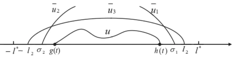
We use u1(t,x) and u2(t,x) to prevent the spreading of two free boundaries respectively, u3(t,x)to control the growth of the solution (see the following Fig. 3.1). We first construct an upper solution to present the spreading ofh(t). Letλ1>0 be the principal eigenvalue of the problem (2.1) when`:= `1, where 0< `1< `∗,φ1is the eigenfunction corresponding toλ1.
Figure 3.1: Three upper solutions u1,u2andu3.
Setσ1(t):= h0+2γ1−γ1e−δt, where 0<δ <λ1,γ1>0 is small such that
h0−γ1 >0, h0+2γ1< `∗, φ01(x)<0 forx∈ [`1−2γ1,`1]. (3.14) Define
u1(t,x):=ε1e−δtφ1(x−σ1(t) +`1) forx∈ [σ1(t)−2γ1,σ1(t)], whereε1>0 is sufficiently small such that
γ1δ≥ −ε1µφ01(`1). (3.15) We now show that (u1,σ1(t)−2γ1,σ1(t)) is an upper solution of the problem (1.1). By (3.14), the definitions ofu1 andφ1we have
u1t−u1xx−(1−u1)
Z
Rk(x−y)u1(t,y)dy
= −δε1e−δtφ1−σ10(t)ε1e−δtφ01−ε1e−δtφ001
−(1−ε1e−δtφ1)
Z
Rε1e−δtk(x−y)φ1(y−σ1(t) +`1)dy
≥ε1e−δt(−δ+λ1)φ1
>0.
(3.16)
Moreover,
σ1(0)>h0, σ1(t)−2γ1≥ g(t) for all t >0, (3.17) and the condition (3.15) implies that
σ10(t) =γ1δe−δt ≥ −µu1x(t,σ1(t)) =−ε1µe−δtφ01(`1). (3.18) If
u(t,σ1(t)−2γ1)< u1(t,σ1(t)−2γ1) =ε1e−δtφ1(`1−2γ1) fort>0, (3.19) then it follows from (3.16)–(3.19) and Remark2.4 that(u1,σ1(t)−2γ1,σ1(t))will be an upper solution of the problem (1.1) when the initial data satisfies
u0(x)< u1(0,x) forx∈ (h0−γ1,h0). (3.20) Then by the comparison principle Lemma2.3we have
h(t)<σ1(t) for allt>0. (3.21) Similarly, we define an upper solutionu2to prevent the spreading of g(t)as follows:
σ2(t):=−h0−2γ2+γ2e−δt, u2(t,x):=ε2e−δtφ1(x−σ2(t)−`1),
forx ∈[σ2(t),σ2(t) +2γ2], whereγ2 >0 is small such that
−h0+γ2<0, −h0−2γ2> −`∗, φ01(x)>0 forx∈[−`1,−`1+2γ2], (3.22) and ε2 > 0 small satisfyingδγ2 ≥ µε2φ01(−`1). Then (u2,σ2(t),σ2(t) +2γ2)will be an upper solution when
u(t,σ2(t) +2γ2)<u2(t,σ2(t) +2γ2) =ε2e−δtφ1(−`1+2γ2) fort >0 (3.23) and
u0(x)<u2(0,x) forx∈ [−h0,−h0+γ2]. (3.24) Therefore, Lemma2.3implies that
g(t)>σ2(t) for all t>0. (3.25) We finally construct the third upper solutionu3 to control the growth of the solution and ensure (3.19) and (3.23). Define
u3(t,x):=ε3e−δtφ2(x), x ∈[−`2,`2],
where ε3 > 0 is very small,φ2(x)is the eigenfunction of the problem (2.1) with` := `2, and
`2satisfies
max{h0+2γ1,h0+2γ2}< `2 < `∗. (3.26)
This is valid by (3.14) and (3.22). It follows from`2< `∗ that the principal eigenvalueλ2>0.
Moreover, (3.26), the definitions ofσ1andσ2imply that
σ1(t)< `2 and σ2(t)>−`2 for allt ≥0. (3.27)
A direct calculation shows that u3t−u3xx−(1−u3)
Z
Rk(x−y)u3(t,y)dy>ε3e−δt(−δ+λ2)φ2>0 (3.28) provided thatδ< λ2. In addition, when
g(t)>−`2 and h(t)< `2 for allt >0, (3.29)
we have
u3(t,g(t))>0= u(t,g(t)) and u3(t,h(t))>0=u(t,h(t)). (3.30) Therefore, (3.28)–(3.30) imply thatu3is an upper solution when the initial datau0 satisfies
u0(x)<u3(0,x) =ε3φ2(x), x∈ [−h0,h0]⊂[−`2,`2]. (3.31) Hence, it follows from the comparison principle that
u(t,x)<u3(t,x) forx ∈[g(t),h(t)], t >0. (3.32) This can ensure (3.19) and (3.23) when ε3 > 0 is sufficiently small. On the other hand, it follows from the definition of σ1, σ2 and the definition of `2 that (3.21) and (3.25) can ensure (3.29) (so (3.32) holds). To guarantee these conclusions, we now chooseu0(x)sufficiently small such that (3.20), (3.24) and (3.31) hold, thenu1,u2andu3are upper solutions at the same time for small t > 0, by the comparison principle and Lemma 2.3, we conclude that (3.19), (3.23) and (3.29) hold,u1,u2andu3 are upper solutions for allt>0. Therefore, by (3.21), (3.25) and (3.32), we obtain
h∞ <∞, g∞ > −∞ and lim
t→∞ku(t,·)kC([g(t),h(t)]) →0.
Then Lemma3.1implies that vanishing happens.
Lemma 3.6. Let h0< `∗ and u0 ∈X(h0), then u spreads ifµ>0is sufficiently large.
Proof. We first consider the caseku0kL∞([−h0,h0]) ≤1, then we can derive from the comparison principle thatu(t,x)<1 for allt>0 andx∈ [g(t),h(t)].
Direct calculation gives d
dt Z h(t)
g(t) u(t,x)dx=
Z h(t)
g(t) ut(t,x)dx+u(t,h(t))h0(t)−u(t,g(t))g0(t)
=
Z h(t)
g(t)
uxx(t,x) + (1−u)
Z
Rk(x−y)u(t,y)dy
dx
= g
0(t)−h0(t)
µ +
Z h(t) g(t)
(1−u)
Z
Rk(x−y)u(t,y)dydx.
(3.33)
Integrating from 0 tot yields Z h(t)
g(t) u(t,x)dx=
Z h0
−h0u0(x)dx+ g(t)−h(t) +2h0 µ
+
Z t
0
hZ h(t) g(t)
(1−u)
Z
Rk(x−y)u(t,y)dydxi
dt, t≥0.
(3.34)
Since 0<u(t,x)<1 fort >0 andx∈[g(t),h(t)], we have, fort ≥1, Z t
0
hZ h(t) g(t)
(1−u)
Z
Rk(x−y)u(t,y)dydxi dt>0.
Assume h∞ 6= +∞ and g∞ 6= −∞, then Lemma 3.3 implies h∞− g∞ ≤ 2`∗ and limt→∞ku(t,·)kL∞([g(t),h(t)])=0. Lettingt→∞in (3.34) gives
Z h0
−h0u0(x)dx ≤ 2`∗−2h0
µ , (3.35)
this contradicts the assumption onµ.
For the case ku0kL∞([−h0,h0]) > 1, we take u0 = ku0(x)
u0kL∞. Let (u,g,h) be the solution of the problem (1.1) with u0 replaced by u0, then by Remark 2.4 we have that (u,g,h) is a lower solution, so Lemma2.2implies thatg(t)<g(t)andh(t)> h(t)fort>0. On the other hand, by the first case, due toku0kL∞([−h0,h0])= 1 and our assumption onµ, we have limt→∞h(t) = +∞and limt→∞g(t) =−∞. Then spreading happens.
3.2 Sharp threshold
In this section, based on the previous results, we obtain sharp threshold behaviors between spreading and vanishing.
Proof of Theorem1.1. According to Lemma3.3, one can obtain spreading-vanishing dichotomy.
In what follows, we will prove the sharp threshold behaviors.
When h0 < `∗, Lemma3.5implies that in this case vanishing happens for all small σ> 0.
Therefore denote
σ∗ := σ∗(h0,φ):=sup{σ0: vanishing happens for σ∈(0,σ0]} ∈(0,+∞].
Ifσ∗ = +∞, then there is nothing left to prove. So we now supposeσ∗ ∈ (0,+∞). (i) We prove spreading when σ > σ∗. By the definition of σ∗ and spreading-vanishing dichotomy, there is a sequenceσndecreasing toσ∗such that spreading happens whenσ=σn,n=1, 2, . . . For any σ > σ∗, there is n0 ≥ 1 such that σ > σn0. Let (un0,gn0,hn0) be the solution of the problem (1.1) with initial data u0 := σn0φ, then by the comparison principle Lemma2.2, we have[gn0(t),hn0(t)]⊂ [g(t),h(t)]andun0(t,x)≤u(t,x). Hence spreading happens for suchσ.
(ii) We show that vanishing happens whenσ≤ σ∗. The definition ofσ∗ implies vanishing when σ < σ∗. We only need to prove vanishing when σ = σ∗. Otherwise spreading must happen when σ = σ∗, so we can find t0 > 0 such that h(t0)−g(t0) > 2`∗. Due to the continuous dependence of the solution of the problem (1.1) on the initial values, we find that ifε>0 is sufficiently small, then the solution of (1.1) withu0 = (σ−ε)φ, denote by(uε,gε,hε), satisfies
hε(t0)−gε(t0)>2`∗. (3.36) Soh∞−g∞ >2`∗, by this and Lemma3.3, we see that (3.36) implies spreading for(uε,gε,hε), which contradicts the definition of σ∗.
Whenh0 ≥`∗, it follows from Lemma3.4that spreading always happens for any solution of the problem (1.1), soσ∗(h0,φ) =0 for anyφ∈X(h0).
A Appendix
Lemma A.1 (Krein–Rutman, [5, Theorem 2.12]). Suppose that A is a compact linear operator on the ordered Banach space E with positive cone P. Suppose further that P has nonempty interior and that A is strongly positive. The eigenvalue problem Au = µu admits a unique eigenvalue µ1 which has a positive eigenvector u1.
We next prove the existence of the principal eigenvalue and the positive eigenfunction cor- responding to it. One can use the similar method as in [8, Theorem 2.2] to prove the following lemma. Additionally, the existence of eigenvalue for (2.1) is equivalent to the existence of the eigenvalue for
φxx+
Z `
−`k(x−y)φ(y)dy−aφ+λφ=0, x ∈(−`,`), φ(−`) =φ(`) =0,
(A.1)
where a >0 is a constant. However, this problem is the same as the eigenvalue problem (13) in [6].
We now give the idea of the proof which is also similar with Example 1 on page 51 in [17].
Lemma A.2. For any` >0,(2.1)has a unique principal eigenvalueλ1(`)and a positive eigenfunction φ1corresponding toλ1(`).
Proof. It is clear that (2.1) is equivalent to
−φxx−
Z `
−`k(x−y)φ(y)dy+aφ= (λ+a)φ(x), x∈(−`,`), φ(−`) =φ(`) =0,
where the constanta >0 is large and it will be chosen later. We first consider the eigenvalue problem
−φxx−
Z `
−`k(x−y)φ(y)dy+aφ=µφ(x), x∈ (−`,`), φ(−`) =φ(`) =0.
(A.2) Thenλ= µ−a.
To prove the existence of eigenvalue, we define a linear operator Aas follows u= Aφ, φ∈C([−`,`]),
whereuis the solution of linear problem
−uxx−
Z `
−`k(x−y)u(y)dy+au= φ(x), x∈(−`,`), u(−`) =u(`) =0.
(A.3)
We now show that A is well defined. For any φ,u ∈ C([−`,`]), by [8, Proposition 2.1], the problem
−vxx+av=
Z `
−`k(x−y)u(y)dy+φ(x), x ∈(−`,`), v(−`) =v(`) =0
has a unique solution v ∈ C2([−`,`]). Then define an operator F(u) = v, by Schauder fixed point theorem, the problem (A.3) has a solutionu∈C2([−`,`]). Moreover, by Lpestimates or the following method (the proof thatAis strongly positive), one can show that the solution of (A.3) is unique. SoAis well defined.
A maps the bounded set in C([−`,`]) onto bounded set in C2([−`,`]), which is the rel- atively compact set belonging to C([−`,`]) (by the embedding theorem). Therefore, A is a compact operator overC([−`,`]).
Now, setP = closure{v :v ∈ C([−`,`]),v > 0 for x ∈(−`,`)}; int P6=∅. We next show that Ais strongly positive, that is, whenφ∈ P\{θ}, then Aφ∈intP. Assume on the contrary that u reaches a negative minimum at x0, by the boundary condition, we have x0 ∈ (−`,`). Sinceu(x0)<0, we can takea>0 large such that
−uxx(x0)−
Z `
−`k(x−y)u(y)dy+au(x0)<0,
this contradicts the choice ofφ ∈ P\{θ}. Hence u(x) ≥ 0 for all x ∈ (−`,`). Furthermore, we prove that u(x) > 0 for all x ∈ (−`,`). Otherwise, by u ∈ C2 andu ≥ 0, there is some minimum pointx∗ ∈(−`,`)such thatu(x∗) =0 anduxx(x∗)>0, from these we have
−uxx(x∗)−
Z `
−`k(x∗−y)u(y)dy+au(x∗)<0, this is also a contradiction. Therefore,u ∈intP.
By Lemma A.1, Aφ = µφ admits a unique eigenvalue µ1(`) which has a positive eigen- functionφ1∈ Pwithkφ1kL2([−`,`]) =1, so the definition ofAimplies
−(φ1)xx−
Z `
−`k(x−y)φ1(y)dy+aφ1 = 1 µ1(`)φ1.