Unlabeled Compression Schemes Exceeding the VC-dimension

Unlabeled Compression Schemes Exceeding the VC-dimension

D¨om¨ot¨or P´alv¨olgyi^∗ and G´abor Tardos^† December 3, 2018

Abstract

In this note we disprove a conjecture of Kuzmin and Warmuth claiming that every family whose VC-dimension is at mostdadmits an unlabeled compression scheme to a sample of size at mostd. We also study the unlabeled compression schemes of the joins of some families and conjecture that these give a larger gap between the VC-dimension and the size of the smallest unlabeled compression scheme for them.

1 Introduction

Terminology: if S is a subset of the domain of a functionf, then we call the restrictiong=f|_S thetrace off onS and we also callf anextension ofg.

Consider a finite set B, and fix a family F of functions B → {0,1}. For f ∈ F and S ⊆ B we call the trace f|_S a partial function of the family F. These are studied extensively in learning theory, where our goal is to reconstructf|_S from some part of it.

Definition 1 (Littlestone and Warmuth [3]). A (labeled) compression scheme for F is a pair of operations(α, β) such that

• α takes a partial functiong of F as an input (called a labeled sample) and returns a trace of g,

• β takes the output ofα as input and returns an arbitrary function f :B → {0,1},

• β(α(g)) is an extension of g for any partial functiong of F.

That is, instead of f|_S, it is enough to storeα(f|_S) so that we can fully recover the value off overS. The size of the compression scheme (α, β) is the maximum size of the domain ofα(g). We denote by LCS(F) the minimum size of a compression scheme for F.

Remark 2. Notice that it is not required to be able to reconstructS fromα(f|_S).

Remark 3. β(α(f|_S)) is not required to be from F.

∗MTA-ELTE Lend¨ulet Combinatorial Geometry Research Group, Institute of Mathematics, E¨otv¨os Lor´and Uni- versity (ELTE), Budapest, Hungary. Research supported by the Lend¨ulet program of the Hungarian Academy of Sciences (MTA), under grant number LP2017-19/2017.

†Supported by the Cryptography “Lend¨ulet” project of the Hungarian Academy of Sciences and by the National Research, Development and Innovation Office, NKFIH projects K-116769 and SNN-117879.

arXiv:1811.12471v1 [math.CO] 29 Nov 2018

Definition 4 (Vapnik-Chervonenkis [5]). Let F be a family of functions B → {0,1}. We say that F shatters X ⊆B if every function g :X → {0,1} has an extension in F. The VC-dimension of F, VC(F), is defined as the size of the largestX that is shattered by F.

Littlestone and Warmuth [3] observed that LCS(F) ≥ VC(F)/5 always holds but could not give any compression scheme for general families whose size depended only on VC(F). Floyd and Warmuth [1] conjectured that LCS(F) ≤ VC(F) always holds. (There are simple examples that show that this would be sharp.) Warmuth [6] even offered $600 reward for a proof that a compression scheme of sizeO(d) always exists, but this has been proved only in special cases.^∗

In 2015, Moran and Yehudayoff [4] have managed to prove that a compression scheme exists whose size depends only on VC(F), but their bound is exponential in VC(F).

Definition 5 (Kuzmin and Warmuth [2]). An unlabeled compression scheme for F is a pair of operations(α, β) such that

• αtakes a partial functiongwith domainS (called a labeled sample) and returns aα(g)(called the compressed sample), which is a subset ofS,

• β takes the output ofα as input and returns an arbitrary function f :B → {0,1},

• β(α(g)) is an extension of g for any partial functiong of F.

That is, unlike in the case of labeled compression schemes, we do not store the value off on the compressed sample, but only some selected sample points. The size of the unlabeled compression scheme (α, β) is the maximum size of α(g) for any partial functiong. We denote by UCS(F) the minimum size of an unlabeled compression scheme for F. Note that UCS(F) ≥LCS(F) trivially holds.

Kuzmin and Warmuth [2] have proved that UCS(F) ≥ VC(F) and conjectured that equality might hold for every family (a strengthening of the earlier conjecture of Floyd and Warmuth).^†

We disprove this last conjecture in a very weak sense; we exhibit a small family C₅ for which VC(C₅) = 2 but UCS(C₅) = 3. We also discuss possible ways to amplify this gap, but at the moment we do not know any familyF with UCS(F)>VC(F) for which UCS(F)≥4. (Although a computer search could possibly find such a family - we exhibit some likely candidates.)

2 Lower bound for C

Here we define the familyC₅ for which UCS(C₅) = 3>VC(C₅) = 2, and prove these equalities.

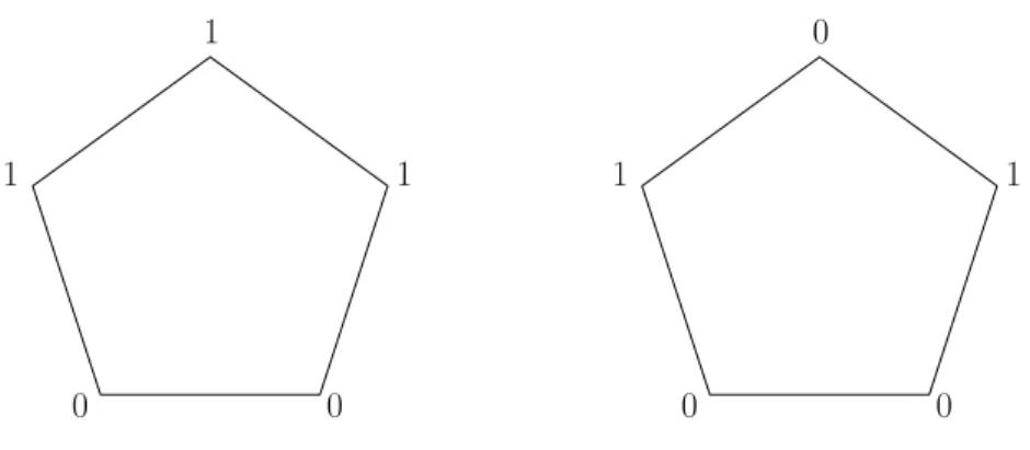
The base set of C₅ is five elements and |C₅|= 10; see Figure 1. We think of the base set B of C₅ as the vertices of a regular pentagon. A 0-1 function on this base set belongs toC5 if and only if it takes the values 1-0-0-1 on some four consecutive vertices.

As we have later found out, this is known in the learning theory literature as ‘Warmuth’s example.’ He constructed it as a simple example of a containment maximal family with VC(C5) = 2 that does not reach the maximal size of such a family given by the Sauer-Shelah lemma, which in this case would beP2

i=0 5 i

= 16.

∗Floyd and Warmuth [1] claimed to have proved it for families of VC-dimensiondwhose size isPd i=0

n i

, i.e., the maximum size allowed by the Sauer-Shelah lemma, but recently an error was discovered in their argument.

†Similarly to the labeled case, they also made a claim about maximum size families, which seems to contain the same error.

1

1 1

0 0

0

1 1

0 0

Figure 1:C5 consists of the 5 rotations of the above sets.

We will use the property that for any subsetS⊂Bof size 3 there are 7 possibilities for the trace f|_S forf ∈C₅. If Sconsists of three consecutive vertices, then f|_S cannot be constant 0, while ifS consists of three non-consecutive vertices the constant 1 trace is not possible. Note that this implies thatC5 shatters no three element set but it shatters all two element sets, so its VC-dimension is 2.

We identify the base set B of C₅ with the residue classes modulo 5, with the neighbors of the vertexi∈B beingi+ 1 and i−1.

Theorem 6. UCS(C₅) = 3.

Proof. It is easy to construct an unlabeled compression scheme of size 3: α can keep the sample points where the value of the function is 1, and the reconstruction function β returns 1 at every place contained in the compressed sample, and 0 everywhere else. Thus, we only need to prove that UCS(C5)≥3.

Suppose by contradiction that there is an unlabeled compression scheme (α, β) of size two.

Let X be a size 3 subset of the domain. As we noted above, there are exactly 7 partial functions g :X → {0,1} of C5. Clearly, α(g) must be a distinct proper subset of X for each. As there are 7 such subsets, we must have a 1-1 correspondence here. In particular, for allY (X, theβ(Y)|_X must be distinct partial functions of C₅.

LetJ be the set of three consecutive positions in the domain andi∈J. Letgbe the constant 0 partial function defined onJ\ {i}andY =α(g). Hereβ(Y)|_J is a partial function ofC5 extending g, so it must be 0 on J \ {i} and 1 on i. Now β({i})|_J must be another partial function of C₅, therefore β({i})|_(J\{i}) cannot be constant 0. A symmetric argument shows that if K is the set of three non-consecutive positions and i∈K, thenβ({i})|_(K\{i}) is not constant 1.

The observations above imply thatβ({i})(i−1) = 1. Indeed, ifβ({i})(i−1) = 0, then applying the observation in the previous paragraph forJ ={i−2, i−1, i}we obtainβ({i})(i−2) = 1 and considering J ={i−1, i, i+ 1} we obtain β({i})(i+ 1) = 1, but this contradicts our observation about K ={i−2, i, i+ 1}. A similar argument showsβ({i})(i+ 1) = 1 as well as β({i})(i−2) = β({i})(i+ 2) = 0. The only remaining value, namely β({i})(i) therefore completely determines β({i}).

Suppose β({i})(i) = 1 holds for at least three different values of i; then it must hold for two consecutive values, say i and i+ 1. This completely determines β({i}) and β({i+ 1}) and these functions coincide on X = {i−2, i, i+ 1} contradicting our observation that for distinct proper subsetsY of X, the β(Y)|_X must also be distinct.

Alternatively we must have β({i})(i) = 0 for at least three different values of i. Then it also holds for two non-consecutive values, say i−1 and i+ 1. This completely determines β({i−1}) and β({i+ 1}) and these functions coincide on X = {i−1, i, i+ 1}, a contradiction again. The contradictions prove the theorem.

Remark 7. Note that in the above proof we have in fact showed that there is no compression scheme already in the case when the sample consists of at most 3 values.

3 Upper bounds for C

’s

In this section we sketch some upper bounds, i.e., give unlabeled compression schemes for certain families. When we receive a samplef|_S, we interpret it as receiving a collection of 0’s and 1’s, and we interpret the compression askeeping some of them (though we only keep the locations, not the values). In the case of C₅, when we receive a sample that contains 3 identical values, then we call them a triple 0 or a triple 1, depending on the value. Recall that a triple 1 can only occur at 3 consecutive positions, and a triple 0 can only occur at 3 non-consecutive positions, so the set of positions determines whether it is a triple 0 or a triple 1.

Definition 8. The joinof two families of functions F ∗ G={(f, g)|f ∈ F, g ∈ G}is a family over the disjoiont union of there base sets where (f, g)(x) = f(x) if x belongs to the base set of F and g(x) if x belongs to the base set of G. When we take the join of several copies of the same family, we use the notationF^∗n=F ∗. . .∗ F

| {z }

ntimes

.

We obviously have VC(F ∗G) = VC(F)+VC(G), but for compression schemes only UCS(F ∗G)≤ UCS(F) + UCS(G) follows from the definition, and equality does not always hold, as the following statement shows. Recall that UCS(C5) = 3 by Theorem 6.

Proposition 9. UCS(C5∗C5)≤5.

Sample Compression Decoding

no triples keep all 1’s kept to 1, rest 0 triple 1 inC₅⁽¹⁾ keep triple and 1’s inC₅⁽²⁾ triple from position, triple 0 inC₅⁽¹⁾ keep triple and 0’s inC₅⁽²⁾ kept in C₅⁽²⁾ same triple 1 inC₅⁽²⁾ keep triple and 0’s inC₅⁽¹⁾ triple from position, triple 0 inC₅⁽²⁾ keep triple and 1’s inC₅⁽¹⁾ kept in C₅⁽¹⁾ opposite

Table 1: Compressing C₅∗C₅.

Proof. For the proof we need to give an unlabeled compression scheme (α, β). There are several possible schemes, one is sketched in Table 1. We write C₅⁽¹⁾ and C₅⁽²⁾ for the base sets of the two copies of C5. The compression α depends on whether there are, and what type of triples in the labeled sample restricted to the base sets of the two copies of C₅. We denote these base sets by C₅⁽¹⁾ and C₅⁽²⁾.

If neither of them contains a triple, we just keep the 1’s in the labeled sample.

If C₅⁽¹⁾ contains a triple 1, butC₅⁽²⁾ does not contain a triple 1, then we still just keep the 1’s.

If C₅⁽¹⁾ contains a triple 0, but C₅⁽²⁾ does not contain a triple 0, then we keep all the 0’s in the labeled sample.

IfC₅⁽²⁾ contains a triple 1, butC₅⁽¹⁾ does not contain a triple 0, then keep the triple 1 fromC₅⁽²⁾, and the 0’s fromC₅⁽¹⁾.

IfC₅⁽²⁾ contains a triple 0, butC₅⁽¹⁾ does not contain a triple 1, then keep the triple 0 fromC₅⁽²⁾, and the 1’s fromC₅⁽¹⁾.

Note that if the compressed sample contains three positions from eitherC₅⁽¹⁾ orC₅⁽²⁾, then those positions formed a triple in the labeled sample and it was a triple 1 in case of three consecutive positions and a triple 0 in case of three non-consecutive positions. This means that the compressed sample determines which one of the five rules was used to obtain it and the decoding β can be constructed accordingly.

Finally, notice that exactly one of the 5 above cases happens for every sample. (Although note that for us it would be sufficient ifat least one of them happened for every sample.)

This raises the question of how UCS(F^∗n) behaves whenn→ ∞. We can prove neither any lower bound that would be better thann·VC(F) for anyFat all (notice that Proposition 9 only provides an upper bound, but we do not know whether in general UCS(F ∗ G) ≥ UCS(F) + UCS(G)−1 holds or not), nor show that UCS(F^∗n)≤(1 +o(1))n·VC(F) for everyF. We make the following conjecture.

Conjecture 10. limn→∞ UCS(C₅^∗n)

n exists and is strictly larger than2.

We can prove that UCS(C₅^∗n)≤2n+ 1 for n≤5. Since the compression schemes are based on similar ideas, we only sketch the scheme forn= 5.

Proposition 11. UCS(C₅^∗5)≤11.

Sample Compression

no triple 1 keep all 1’s

triple 1 in some C₅⁽ⁱ⁾ but no triple 0 anywhere

keep triple 1 in C₅⁽ⁱ⁾ and 0’s in otherC₅^(j)’s

exactly one triple 0 keep 0’s

exactly one triple 1 and least two triple 0’s

fix two triple 0’s and one triple 1;

keep non-central triples and central element of central triple, and 1’s from rest

least two triple 1’s and least two triple 0’s, and fifth does not have ex- actly one 1

keep triple 1’s and central elements of triple 0’s, and 1’s from fifth two triple 1’s and least two triple 0’s,

and fifth has exactly one 1

keep triple 1’s and non-central ele- ments of triple 0’s, and 1 from fifth Table 2: Compressing C₅^∗5.

Proof. We denote the 5 copies of C₅’s by C₅⁽⁰⁾, . . . , C₅⁽⁴⁾, with indexing mod 5.

Among any three positions in a singleC₅⁽ⁱ⁾ there is a unique “central” element: the one that is equidistant from the other two elements. We use that the two non-central elements determine the central element uniquely. Although the central element is not enough to determine the other two elements, it becomes enough once we know whether they are the positions in a triple 0 or a triple 1.

Similarly, among any three distinct setsC₅⁽ⁱ⁾,C₅^(j)andC₅^(k), there is a unique central one, whose index is equidistant (modulo 5) from the other two indices. E.g., from C₅⁽⁰⁾, C₅⁽²⁾ and C₅⁽³⁾ the central one is C₅⁽⁰⁾, while from C₅⁽⁰⁾,C₅⁽³⁾ and C₅⁽⁴⁾ the central one is C₅⁽⁴⁾. We use again that the non-central copies determine the central one uniquely.

The compression algorithm is sketched in Table 2. This Table needs to be interpreted in a similar fashion as Table 1, this time we omit the lengthy description of the case analysis. Note that for some labeled samples there are more rules to choose from for the compression – in this case, we pick arbitrarily. It is important, however that there is always at least one rule that applies.

We have also omitted the decompression rules, as the compressed sample always determines which rule was used to obtain it. To prove this statement, notice that we only keep three position of the sameC₅⁽ⁱ⁾ if they form a triple in the labeled sample. If the first rule is used, no triple is kept.

In case the second or third rule is used, a single triple 1 or triple 0 is kept, respectively. If the fourth rule is used, then two triples are kept, not both triple 1’s. Finally if either of the last two rules are used, then at least two triple 1’s are kept. The compressed sample produced by the last two rules are distinguished by the number of elements kept in the setsC₅⁽ⁱ⁾: if it is 3 + 3 + 2 + 2 + 1 in some order, then the last rule was used, otherwise the fifth rule. Once we know which rule produced the compressed sample the decoding can be done accordingly.

4 Further results

In this section we mention some further results. We start by defining some further families.

C₅⁻ is obtained fromC₅ by deleting one function. Because of the symmetry, it does not matter which one, so we delete the function 0-1-1-1-0. Here we represent functions by the sequence of their values on 0, 1, 2, 3, 4. In this family, still any two positions can take any values (4 possibilities each), but for some triples we have only 6 possibilities (instead of 7).

C4 is the restriction of C5 to four elements of the base set. Again, by symmetry it does not matter which four, so we delete the central element 2. This is useful, because this way C4 also becomes a restriction ofC₅⁻.

Proposition 12. UCS(C4) = UCS(C₅⁻) = 2.

Proof. The lower bounds follow from 2 = VC(C4)≤UCS(C4) ≤UCS(C₅⁻). For the upper bound, we need to give a compression scheme of size two forC₅⁻. A possible algorithm is sketched in Table 3. Here we list the decoding of compressed samples only. We maintain a symmetry for the reflection to the central element: If the compressed sample B is obtained from another compressed sample Aby reflection, then the decodingβ(B) is also obtained fromβ(A) the same way. Accordingly, we only list one of A and B in the Table. We omit the lengthy case analysis of why this compression scheme works.

Now we continue by definining two more families.

Compression Decoding

∅ 1-0-0-0-1

x-.-.-.-. 0-0-1-0-1

.-x-.-.-. 1-1-0-0-1

.-.-x-.-. 1-0-1-0-1

x-x-.-.-. 0-1-0-0-1

x-.-x-.-. 0-1-0-0-1

x-.-.-x-. 0-0-1-1-1

x-.-.-.-x 0-1-0-1-0

.-x-x-.-. 1-1-1-0-0

.-x-.-x-. 0-1-0-1-0

Table 3: Compressing C₅⁻; elements of the compressed sample are marked with an x.

P(k) is the family of all 2^k boolean functions on a base set ofk elements. Notice that P(k) = P(1)^∗k. As P(k) shatters its entire base set, we have VC(P(k)) =k. We also have UCS(P(k)) =k as VC(P(k)) ≤ UCS(P(k)) and UCS(P(k) ≤ k is shown by the simple unlabeled compression scheme that keeps the 1’s in the labeled sample. On the other hand, LCS(P(k)) can be smaller, e.g., LCS(P(2)) = 1.

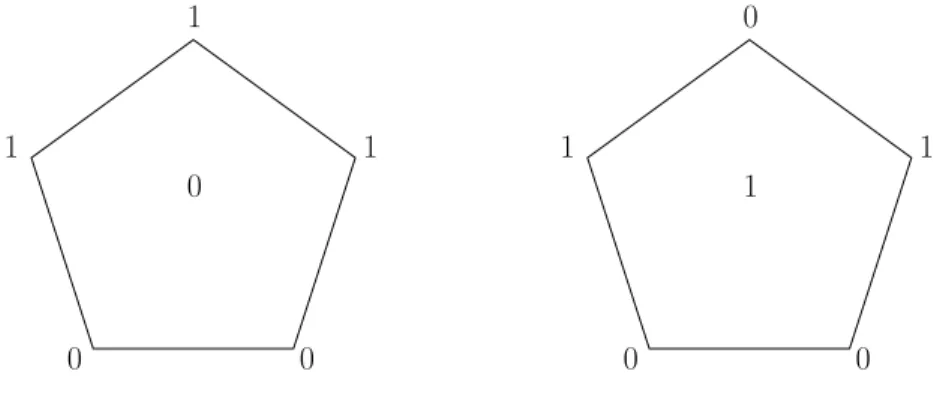
W₆ is a symmetrizing extension of C₅, with the same number of functions, but one more base element. One can obtain it from C5 by adding an extra element to the base and extending each function in the family to the new element such that the function has three zeros and three ones.

Figure 2 depict two functions of W₆. The other eight functions are the rotations of these two. In the family W₆ the extra element plays no special role, in fact, W₆ is two-transitive, i.e., any pair of elements of its base set can be mapped to any other pair of elements with an automorphism. If we convert the functions of W₆ to 3-element sets, we get the unique 2−(6,3,2) design. SinceW₆ is an extension of C₅, VC(C₅)≤VC(W₆) and UCS(C₅) ≤UCS(W₆) – it is easy to check that we have equality in both cases, i.e., VC(W6) = 2 and UCS(W6) = 3.

1

1 1

0 0

0

0

1 1

0 0

1

Figure 2: W₆ consists of the 5 rotations of the above sets.

Some further non-trivial upper bounds can be obtained for the joins involving these families.

Proposition 13. UCS(W₆∗P(1)) = 3.

Sample Compression Decoding extra is not 1 keep 1’s ofW₆ kept 1, others 0 extra is 1 and triple 0 keep triple 0 kept 0, others 1

extra is 1, no triple 0 keep extra and 0’s extra 1, rest of kept 0, others 1 Table 4: Compressing W₆∗P(1).

Proof. The compression algorithm is sketched in Table 4, with ‘extra’ denoting the only bit of the base set ofP(1).

Note thatC5∗P(1) is obtained fromW6∗P(1) by restricting the base set and such a restriction cannot increase the value of UCS, so this also implies UCS(C5∗P(1)) = 3. From this we can easily get another proof for UCS(C₅∗C₅)≤5 as follows. We haveC₅⊂P(1)∗C₄, thus UCS(C₅∗C₅)≤ UCS(C5∗P(1)∗C4)≤UCS(C5∗P(1)) + UCS(C4)≤3 + 2, using Proposition 12.

Proposition 14. UCS(W₆∗W₆)≤5.

Proof. This compression goes similarly to the one presented in Table 1 forC5∗C₅. In fact, we can use exactly the same compression scheme unless we get two triples in bothW₆’s, i.e., a labeled sample that contains all 12 elements of the base. There are 10·10 = 100 possibilities for such a sample, and for each we can pick a compression that keeps at least 4 elements from at least one of the two copies ofW₆, as these were not used yet. There are ⁶₅

· ⁶₀ + ⁶₄

· ⁶₁ + ⁶₄

· ⁶₀ + ⁶₀

· ⁶₄ + ⁶₁

· ⁶₄ + ⁶₀

· ⁶₅

= 222 such possible compressed samples, we can use a distinct one for each of the 100 problematic labeled samples. This makes the decoding possible.

We end by a summary of the most important questions left open.

Summary of main open questions

• Is UCS(F)−VC(F) bounded?

• Is UCS(F ∗ G)≥UCS(F) + UCS(G)−1?

• How does UCS(C₅^∗n) behave? Does lim UCS(n∗ F)/n exist?

• Is there akfor every F such that UCS(F ∗P(k)) = VC(F) +k?

Remarks and acknowledgment

We would like to thank Tam´as M´esz´aros, Shay Moran and Manfred Warmuth for useful discus- sions and calling our attention to new developments.

References

[1] S. Floyd and M. K. Warmuth, Sample compression, learnability, and the Vapnik-Chervonenkis dimension, in Machine Learning, 21(3):269–304, 1995.

[2] D. Kuzmin and M. K. Warmuth, Unlabeled Compression Schemes for Maximum Classes, in Proceedings of the 18th Annual Conference on Computational Learning Theory (COLT 05), Bertinoro, Italy, pp. 591–605, June 2005.

[3] N. Littlestone and M. K. Warmuth, Relating data compression and learnability. Unpublished manuscript, ob- tainable athttp://www.cse.ucsc.edu/~manfred, June 10 1986.

[4] S. Moran and A. Yehudayoff, Sample compression schemes for VC classes, to appear in the Journal of the ACM.

[5] V. N. Vapnik, A. Ya. Chervonenkis, On the Uniform Convergence of Relative Frequencies of Events to Their Probabilities, Theory of Probability & Its Applications. 16(2):264-280, 1971.

[6] M. K. Warmuth, Compressing to VC dimension many points, in Proceedings of the 16th Annual Conference on Learning Theory (COLT 03), Washington D.C., USA, August 2003. Springer. Open problem.https://users.

soe.ucsc.edu/~manfred/pubs/open/P1.pdf.