In 1988, Falconer proved that, for given matrices, the Hausdorff dimension of the self-affine set is the affinity dimension for Lebesgue almost every translation vectors

DIMENSION OF SELF-AFFINE SETS FOR FIXED TRANSLATION VECTORS

BAL ´AZS B ´AR ´ANY, ANTTI K ¨AENM ¨AKI, AND HENNA KOIVUSALO

Abstract. An affine iterated function system is a finite collection of affine invertible contractions and the invariant set associated to the mappings is called self-affine. In 1988, Falconer proved that, for given matrices, the Hausdorff dimension of the self-affine set is the affinity dimension for Lebesgue almost every translation vectors. Similar statement was proven by Jordan, Pollicott, and Simon in 2007 for the dimension of self-affine measures. In this article, we have an orthogonal approach. We introduce a class of self-affine systems in which, given translation vectors, we get the same results for Lebesgue almost all matrices. The proofs rely on Ledrappier-Young theory that was recently verified for affine iterated function systems by B´ar´any and K¨aenm¨aki, and a new transversality condition, and in particular they do not depend on properties of the Furstenberg measure. This allows our results to hold for self-affine sets and measures in any Euclidean space.

1. Introduction

For a non-singulard×dmatrix A∈GL_d(R) and a translation vector v∈R^d, let us denote the affine mapx7→Ax+v byf =f(A, v). LetA= (A1, . . . , AN)∈GLd(R)^N be a tuple of contractive non-singulard×dmatrices and letv= (v₁, . . . , v_N)∈(R^d)^N be a tuple of translation vectors. Here and throughout we assume thatN ≥2 is an integer. The tuple ΦA,v= (f1, . . . , fN) obtained from the affine mappingsf_i =f(A_i, v_i) is called the affine iterated function system (IFS). Hutchinson [19] showed that for each ΦA,v there exists a unique non-empty compact setE =EA,v such that

E=

N

[

i=1

fi(E).

The setEA,vassociated to an affine IFS ΦA,v is calledself-affine. In the special case where each of the linear mapsA_i is a scalar multiple of an isometry, we call Φ_A,v a similitude iterated function system and the set EA,v self-similar.

The dimension theory of self-similar sets satisfying a sufficient separation condition was completely resolved by Hutchinson [19]. Without separation, i.e. when the imagesfi(E) and fj(E) can have severe overlapping, the problem is more difficult. The most recent progress in this direction is by Hochman [15, 16]. Among other things, he managed to calculate the Hausdorff dimension of a self-similar set on the real line under very mild assumptions.

In contrast, the dimension theory of self-affine sets and measures is still far from being fully understood. Traditionally, while working on the topic, it has been common to focus on specific subclasses of self-affine sets, for which more methods are available. One such standard subclass is that of self-affine carpets. In this class special relations between the affine maps are imposed, which makes the structure of the self-affine set more tractable. For recent results for self-affine carpets, see [13, 14, 25]. Another method of study and a class of self-affine sets to which it applies was introduced by Falconer [8] and later extended by Solomyak [32]. They proved that for a fixed matrix tupleA= (A₁, . . . , A_N)∈GL_d(R)^N, with the operator normskA_ik strictly less than 1/2,

Date: February 6, 2018.

2010Mathematics Subject Classification. Primary 37C45; Secondary 28A80.

Key words and phrases. Self-affine set, self-affine measure, Hausdorff dimension.

BB and HK were partially supported by Stiftung Aktion ¨Osterreich Ungarn (A ¨OU) grants 92¨ou6. BB acknowledges the support from the grant OTKA K104745, OTKA K123782, NKFI PD123970 and the J´anos Bolyai Research Scholarship of the Hungarian Academy of Sciences, and HK from EPSRC EP/L001462 and Osk. Huttunen foundation.

1

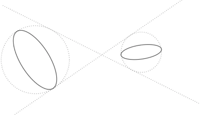
Figure 1. The picture illustrates three example cases where some other covering is more optimal than the one obtained from (1.1). From left to right: ellipses have severe overlapping, the ellipsis does not containEall the way, and ellipses are badly aligned.

the Hausdorff dimension of the self-affine set EA,v, dimH(EA,v), is the affinity dimension of A, dim_aff(A), for L^dN-almost all v ∈ (R^d)^N. Here L^d is the d-dimensional Lebesgue measure and the affinity dimension, defined below, is a number depending only onA. A similar result, due to Jordan, Pollicott, and Simon [20], also holds for self-affine measures.

Let us next give an intuitive explanation for Falconer’s result. It is easy to see that E =

∞

\

n=1

[

i1,...,in∈{1,...,N}

fi1◦ · · · ◦fin(B(0, R)), (1.1) where B(0, R) is the closed ball centered at the origin with radius R = maxi∈{1,...,N}|v_i|/(1− maxi∈{1,...,N}kA_ik) > 0. Since we are interested in the dimension of E we may, by rescaling if necessary, assume that R = 1. We immediately see from (1.1) that for each fixed n the sets fi1 ◦ · · · ◦fin(B(0,1)) form a cover for the self-affine set. For any A∈GLd(R), let 1> α1(A)≥

· · · ≥α_d(A) >0 be the lengths of the principal semiaxes of the ellipse A(B(0,1)). Observe that f_i1◦ · · · ◦f_in(B(0,1)) is a translated copy ofA_i1· · ·A_in(B(0,1)). To find the Hausdorff dimension of E, it is necessary to find optimal covers forE. Natural candidates for such covers come immediately from (1.1). In R², we need approximately α₁(A_i1· · ·A_in)/α₂(A_i1· · ·A_in) many balls of radius α2(Ai1· · ·Ain) to coverfi1 ◦ · · · ◦fin(B(0, R)). By the definition of the s-dimensional Hausdorff measure H^s, it follows that

H^s(E). lim

n→∞

X

i1,...,in∈{1,...,N}

α₁(A_i1· · ·A_in)

α2(Ai1· · ·Ain)α₂(A_i1· · ·A_in)^s

= lim

n→∞

X

i1,...,in∈{1,...,N}

α₁(A_i1· · ·A_in)α₂(A_i1· · ·A_in)^s−1. The singular value pressure PA of A in this case is

PA(s) = lim

n→∞

1

nlog X

i1,...,in∈{1,...,N}

α1(Ai1· · ·Ain)α2(Ai1· · ·Ain)^s−1.

For the complete definition, see (2.3). The functions7→P_A(s) is strictly decreasing and it has a unique zero. If PA(s) < 0, then the sum above is strictly less than one for all large enough n. Therefore, defining dim_aff(A) to be the minimum of 2 and s for which P_A(s) = 0, we have dimH(EA,v) ≤ dimaff(A) for all v ∈ (R²)^N. The question then becomes, when are the covers obtained in this way optimal. It is easy to find situations in which some other cover is more efficient;

see Figure 1. Intuitively, since the role of the translation vector is to determine the placement of the ellipses, Falconer’s result asserts that one never encounters these situations with a random choice of translation vectors.

Recently, there is an increasing amount of activity in studying the case of general affine iterated function systems, based neither on the strict structure of the self-affine carpets nor Lebesgue generic translation vectors. Morris and Shmerkin [27] proved that dimH(EA,v) = dimaff(A), under both an exponential separation condition on the matrices, that was first introduced by Hochman and Solomyak [17], and a separation condition on the IFS. An interesting observation is that the result of Hueter and Lalley [18] can be covered as a special case of [27, Theorem 1.3], and hence, the

techniques used by Morris and Shmerkin give it an alternative proof. In particular, if a matrix tuple in GL2(R)^N satisfy the dominated splitting condition (for a precise definition, see §2) and the strong separation condition on the projective line, then it satisfies the exponential separation condition. Since both the dominated splitting and strong separation conditions are open properties (i.e. if a matrix tuple satisfies it, then it holds in its open neighbourhood), there exists an open set, where the exponential separation condition holds in GL2(R)^N. In general, the exponential separation condition holds on a denseG_δσ set in GL₂(R)^N, but it is unknown whether it is satisfied by measure theoretically generic tuples of matrices.

Morris and Shmerkin need to further assume that either a so called bunching condition holds, or argue through an application of a result of Rapaport [29], which assumes that the dimension of the Furstenberg measure (for the definition, see §3) is large compared to the Lyapunov dimension.

Similarly, Falconer and Kempton [10] prove that dim_H(E_A,v) = dim_aff(A), assuming a positivity condition on the matrices, a separation condition on the IFS, and a condition on the dimension of the Furstenberg measure. Both the results of Morris and Shmerkin, and of Falconer and Kempton, rely on calculating the dimension of the Furstenberg measure and can, with the current knowledge of Furstenberg measures, only be applied in the plane.

Our approach combines Ledrappier-Young theory, which was recently proven to hold for many measures on self-affine sets by B´ar´any and K¨aenm¨aki [3, 5], and a transversality argument. Our results are a natural counterpart to Falconer’s result [8]: we fix the tuple of translation vectors and investigate the dimension for different choices of matrix tuples. In the same vein as with the intuitive explanation of Falconer’s result, one expects that, keeping the centers of the ellipses fixed, a small random change in the shape of the ellipses guarantees that the covers obtained from (1.1) are optimal. Indeed, in the main results of the paper, Theorems A and B, we fix a tuple of distinct translation vectors v∈(R^d)^N, and show that dimH(EA,v) = dimaff(A) for L^d2N-almost allA in a large open set of matrix tuples. Notably, a separation condition holds in this open set and for d≥3 we also need to impose a totally dominated splitting condition (see (2.6)) on the matrices.

The sharpness and possible extensions are discussed in Remarks 2.2 and 3.6.

A key ingredient in the proof is a verifiable transversality condition, which we call the modified transversality condition, which we introduce in a general setting in §3. This condition allows us to calculate the Hausdorff dimension of self-affine sets and measures through the Ledrappier- Young formula. Therefore, in order to prove the main theorems it suffices to verify the modified transversality condition in the particular setups. We note that the method for calculating dimensions of measures on self-affine sets, as described in§3, is rather general, and immediately applies to give stronger results, if there are improvements on the existing results on Ledrappier-Young theory and transversality arguments that the proofs rely on. Another curious feature of our results is that the planar case is different from the higher dimensional case both in statement and in proof; see Remark 2.2 for comparison. The planar case is stated in Theorem A and the higher dimensional case in Theorem B.

Since our proofs do not rely on dimension estimates for the Furstenberg measures, our results hold not only for dimensions of self-affine sets but also self-affine measures, and for any ambient space R^d, not just in the plane. Furthermore, our results hold for an open set of matrix tuples even in parts of the space where the Furstenberg measure has a small dimension compared to the Lyapunov dimension, namely, when the bunching condition does not hold; see Remark 2.3. This is in stark contrast to the earlier works.

The remainder of the paper is organized as follows. In§2, we give a detailed explanation of the setting and state our main results. We explore in §3 how the Hausdorff dimension of an ergodic measure satisfying the Ledrappier-Young formula can be calculated under a modified self-affine transversality condition. In§4, we prove an analogous result for self-affine sets. Finally, the proof of Theorem A is given in§5 and Theorem B is proved in§6.

2. Preliminaries and statements of main results

Let Σ be the set of one-sided words of symbols {1, . . . , N} with infinite length, i.e. Σ = {1, . . . , N}^N. Let us denote the left-shift operator on Σ byσ. Let the set of words with finite length be Σ∗ =S∞

n=0{1, . . . , N}ⁿwith the convention that the only word of length 0 is the empty word∅. The set Σn={1, . . . , N}ⁿ is the collection of words of length n. Denote the length ofi∈Σ∪Σ∗ by

|i|, and for finite or infinite wordsi and j, let i∧jbe their common beginning. The concatenation of two wordsi andjis denoted by ij. We define the cylinder sets of Σ in the usual way, that is, by setting

[i] ={j∈Σ :i∧j=i}={ij∈Σ :j∈Σ}

for alli∈Σ∗. For a wordi= (i1, . . . , in) with finite length letfi be the compositionfi1 ◦ · · · ◦fin

andA_i be the product A_i1· · ·A_in. For i∈Σ∪Σ∗ and n <|i|, let i|_n be the first n symbols ofi.

Let i|₀ =∅,A_∅ be the identity matrix, and f_∅ be the identity function. Finally, we define the natural projection π=πA,v: Σ→EA,v by setting

π(i) =

∞

X

k=1

Ai|_k−1vik (2.1)

for all i∈Σ. Note thatE =S

i∈Σπ(i).

Denote by α_i(A) thei-th largest (counting with multiplicity) singular value of a matrix A∈ GL_d(R), i.e. the positive square root of the i-th eigenvalue of AA^T, where A^T is the transpose of A. We note that α1(A) is the usual operator norm kAk induced by the Euclidean norm on R^d and α_d(A) is the mininorm m(A) = kA⁻¹k⁻¹. We say that A is contractive if kAk < 1.

For a given tuple A = (A₁, . . . , A_N) ∈ GL_d(R)^N we also set kAk = maxi∈{1,...,N}kA_ik and m(A) = mini∈{1,...,N}m(A_i). Following Falconer [8], we define thesingular value functionϕ^s of a matrixA by setting

ϕ^s(A) =

(α1(A)· · ·α_bsc(A)α_dse(A)^s−bsc, if 0≤s≤d,

|detA|^s/d, ifs > d.

The singular value function satisfies

ϕ^s(AB)≤ϕ^s(A)ϕ^s(B)

for all A, B∈GLd(R). Moreover, if (A1, . . . , AN)∈GLd(R)^N, then

ϕ^s(A_i)m(A)^δ|i|≤ϕ^s+δ(A_i)≤ϕ^s(A_i)kAk^δ|i| (2.2) for all i∈Σ∗ and s, δ≥0.

For a tupleA= (A1, . . . , A_N)∈GL_d(R)^N of contractive non-singulard×dmatrices the function P_A: [0,∞)→Rdefined by

P_A(s) = lim

n→∞

1

nlog X

i∈Σn

ϕ^s(A_i) (2.3)

is called the singular value pressure. It is well-defined, continuous, strictly decreasing on [0,∞), and convex between any two integers. Moreover,P_A(0) = logN and lims→∞P_A(s) =−∞. Let us denote by dim_affAthe minimum of dand the unique root of the singular value pressure function and call it theaffinity dimension.

Ifµis a Radon measure on R^d, then the upper and lower local dimensions ofµat x are defined by

dim_loc(µ, x) = lim sup

r↓0

logµ(B(x, r))

logr and dim_loc(µ, x) = lim inf

r↓0

logµ(B(x, r)) logr , respectively. The measureµ isexact-dimensional if

ess infx∼µdim_loc(µ, x) = ess sup_x∼µdimloc(µ, x).

In this case, the common value is denoted by dimµ. The above quantities are naturally linked to set dimensions. For example, thelower Hausdorff dimension of the measureµ is

dim_Hµ= ess infx∼µdim_loc(µ, x) = inf{dim_HA:Ais a Borel set with µ(A)>0}.

Here dim_HA is the Hausdorff dimension of the setA. For more detailed information, the reader is referred to [9].

Fix a probability vectorp= (p₁, . . . , p_N)∈(0,1)^N and denote the productp_i1· · ·p_in byp_i for all finite wordsi= (i1, . . . , in). Letνp be the corresponding Bernoulli measure on Σ. It is uniquely defined by setting ν_p([i]) =p_i for all i∈Σ∗. It is easy to see thatν_p is σ-invariant and ergodic.

We say thatν on Σ is a step-n Bernoulli measure if it is a Bernoulli measure on (Σ_n)^N for some probability vector from (0,1)^Nn. Furthermore, we say that a measure ν on Σ is quasi-Bernoulli if there is a constant C≥1 such that

C⁻¹ν([i])ν([j])≤ν([ij])≤Cν([i])ν([j]) for all i,j∈Σ∗. Theentropy of aσ-invariant measure ν on Σ is

hν =− lim

n→∞

1 n

X

i∈Σn

ν([i]) logν([i]). (2.4)

Note that the entropy of a Bernoulli measureν_p is given by h_p=−P_N

i=1p_ilogp_i.

Ifν_p is a Bernoulli measure and Φ_A,v is an affine iterated function system, then the push-down measureµ_A,v,p=π_A,vν_p =ν_p◦(π_A,v)⁻¹ is calledself-affine. It is well known that the self-affine measure µ=µA,v,p satisfies

µ=

N

X

i=1

pifiµ.

We say thatA∈GL_d(R)^N satisfies thetotally dominated splitting conditionif there exist constants C≥1 and 0< τ <1 such that for everyi∈ {1, . . . , d−1} either

αi+1(A_i)

α_i(A_i) ≤Cτ^|i| (2.5)

for everyi∈Σ∗ or

αi+1(A_i)

α_i(A_i) > C⁻¹

for everyi∈Σ∗. By Bochi and Gourmelon [7, Theorem B], the set

D={A∈GLd(R)^N : (2.5) holds for every i∈ {1, . . . , d}}. (2.6) is an open subset ofGL_d(R)^N.

Ifν is an ergodic probability measure on Σ, then, by Oseledets’ theorem, there exist constants 0< χ₁(A, ν)≤ · · · ≤χ_d(A, ν)<∞ such that

χi(A, ν) =− lim

n→∞

1

nlogαi(Ai1· · ·Ain) (2.7) for ν-almost every i ∈ Σ. The numbers χi(A, ν) are called the Lyapunov exponents of A with respect toν. The Lyapunov exponents of Awith respect to a Bernoulli measureν_p are denoted by χi(A,p). Furthermore, let us define the Lyapunov dimension ofν by

dim_Lν = min

k∈{0,...,d}

k+hν −Pk

j=1χj(A, ν) χk+1(A, ν) , d

.

The Lyapunov dimension of the projected measureπνonE_A,vis defined by setting dim_Lπν= dim_Lν.

K¨aenm¨aki [21, Theorems 2.6 and 4.1] proved the existence of ergodic equilibrium states. If s= dim_affA≤d, then an ergodic s-equilibrium stateµof A on Σ is defined by the equality

h_µ=−lim_n¹ X

i∈Σn

µ([i]) logϕ^s(A_i) =

bsc

X

j=1

χ_j(A, µ) + (s− bsc)χ_dse(A, µ). (2.8)

Here the second equality follows from Kingman’s ergodic theorem. It is easy to see that such an s-equilibrium state is a measure of maximal Lyapunov dimension.

B´ar´any and K¨aenm¨aki recently proved in [5, Theorem 2.3] that the self-affine measureµ_A,v,p is exact-dimensional regardless of the choices ofA,v, andp provided that all the corresponding Lyapunov exponents are distinct. Furthermore, they showed that ifAsatisfies the totally dominated splitting condition, then the image of any quasi-Bernoulli measure under π_A,v is exact-dimensional regardless of the choice ofv; see [5, Theorem 2.6].

Let us next state the main results of the article. Let L^dbe the d-dimensional Lebesgue measure and dim_M be the upper Minkowski dimension. We definekvk= maxi∈{1,...,N}|v_i|and recall that kAk= maxi∈{1,...,N}kA_ik.

Theorem A. Suppose that v= (v1, . . . , vN)∈(R²)^N is such that vi 6=vj for i6=j and A_v=

A∈GL2(R)^N : 0<max

i6=j

kA_ik+kA_jk

|v_i−vj| · kvk 1− kAk <

√ 2 2

. (2.9)

Then

dimHEA,v= dimMEA,v= dimaffA

forL^4N-almost all A∈ A_v. Moreover, for every probability vector p∈(0,1)^N the corresponding self-affine measure µ=µ_A,v,p satisfies

dimµ= dimLµ= min

hp

χ₁(A,p),1 +hp−χ1(A,p) χ₂(A,p)

for L^4N-almost allA∈ A_v.

Note that matrix tuples inA_v are contractive. In higher dimensions, our result is the following.

Theorem B. Suppose thatd∈N is such that d≥3,v= (v1, . . . , v_N)∈(R^d)^N is such that vi 6=vj

for i6=j, and A⁰_v=

A∈GLd(R)^N : 0<max

i6=j

kA_ik+kA_jk

|v_i−vj| · kvk

1− kAk < 2

√ 3 −1

. (2.10)

Then for every probability vector p ∈ (0,1)^N the corresponding self-affine measure µ = µ_A,v,p satisfies

dimµ= dim_Lµ= min

k∈{0,...,d}

k+hp−Pk

j=1χj(A,p) χk+1(A,p) , d

for L^d2N-almost allA∈ A⁰_v. Moreover,

dimHµA = dimHEA,v= dimMEA,v = dimaffA

forL^d2N-almost all A∈ A⁰_v∩ D, whereD is as in (2.6)and µA is an ergodic s-equilibrium state of A for s= dim_affA.

Let us show that the equilibrium states in Theorem B are quasi-Bernoulli.

Lemma 2.1. For L^d2N-almost every A ∈ A⁰_v∩ D the unique s-equilibrium state of A is quasi- Bernoulli fors= dim_aff(A).

Proof. By [23, Propositions 3.4 and 3.6], for L^d2N-almost every A∈GL_d(R)^N, the s-equilibrium state of A for s= dim_affA is unique and satisfies the following Gibbs property: there exists a constantC≥1 such that

C⁻¹ϕ^s(A_i)≤µ([i])≤Cϕ^s(A_i)

for all i∈Σ∗. By [7, Theorem B] and [12, Lemma 2.1], for each A ∈ D, there exists a constant C⁰>0 such that

C⁰ϕ^s(A_i)ϕ^s(A_j)≤ϕ^s(A_ij)

for all i,j∈Σ∗. The statement of the lemma follows.

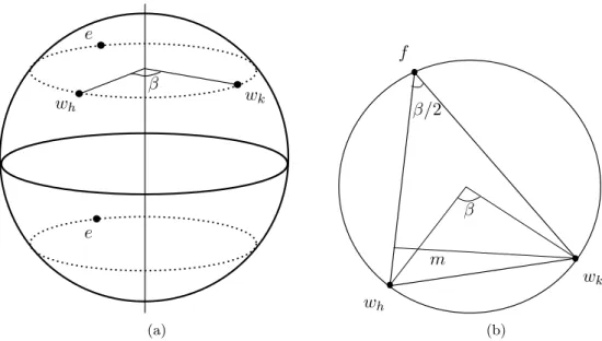
Figure 2. The condition (2.9) requires that the images of the unit ball underfi are separated away from each other as in the picture: if the ellipses are rotated around their centers, they still stay inside a cone having an angle at mostπ/2.

Remark 2.2. We emphasize that the methods used to prove Theorems A and B are significantly different. At first, the higher dimensional exact dimensionality result for quasi-Bernoulli measures (the Ledrappier-Young formula to be more precise) of B´ar´any and K¨aenm¨aki [5] requires the totally dominated splitting condition, which is why we restrict our matrix tuples to the setD. Very recently, Feng [personal communication] has informed the authors that the Ledrappier-Young formula holds also without totally dominated splitting. By relying on this, one could improve Theorem B by replacingA⁰_v∩ D byA⁰_v. Secondly, the transversality argument used in the higher dimensional case is different from the two-dimensional case. Curiously, the higher dimensional transversality argument requires the dimension to be at least three, so it cannot be used in the two-dimensional case. This difference is also the reason why we use different upper bounds in the definitions ofA_v andA⁰_v. Currently we do not know if the upper bound 2/√

3−1 used in (2.10) can be replaced by the upper bound√

2/2 used in (2.9). The sharpness of the methods used in our proofs is discussed in Remark 3.6.

Remark 2.3. Many of the recent works on dimensions of self-affine sets and measures (see e.g.

[5, 6, 27, 29]) rely on properties of the Furstenberg measure (for definitions, see§3) and on the exceptional sets of the dimension of orthogonal projections. We remark that the result of B´ar´any and Rams [6] is the first result in the direction of almost every matrices. However, Theorem A covers situations that cannot be addressed by using this approach. Even though the condition (2.9) is rather restrictive (for example, we will see in Lemma 2.4 that it implies that the images f_i(E) are disjoint, i.e. ΦA,v satisfies thestrong separation condition) Theorem A introduces a checkable condition for an affine iterated function system to satisfy the desired dimension result. This is in contrast to, for example, [5, Corollaries 2.7 and 2.8] where the claim for the self-affine measureµin Theorem A holds provided that the strong separation condition holds and the dimension of µdoes not drop when projected to orthogonal complements of Furstenberg typical lines. The condition (2.9) can be illustrated via Lemma 3.7 as in Figure 2.

We will next exhibit an open set of matrices that satisfy the assumptions of Theorem A, but do not satisfy the projection condition of [5]. Consider an affine iterated function system consisting of three mappingsx7→A_ix+v_i. Let the translation vectors v_i be equidistributed on the unit circle, that is,|v_i|= 1 and |v_i−vj|=√

3 for alli6=j. It is easy to see that ifkA_ik<√

6/(4 +√ 6) =:η for alli, thenA∈ A_v. Since η >1/3 we find an open set of three matrices such that all elements are strictly positive, the Furstenberg measure is supported on a Cantor set having dimension less than 1/2, and the affinity dimension is between 1 and 3/2. Recalling [5, Corollary 2.9], we see that this case does not satisfy the projection condition. Also, this example is outside of the scope of Morris and Shmerkin [27, Theorems 1.2 and 1.3], since the affinity dimension is less than 3/2

and, as the affinity dimension is strictly larger than the dimension of the Furstenberg measure, the bunching condition does not hold either.

In the next lemma, we note that the strong separation condition follows from the conditions (2.9) and (2.10). Denote byO(d) the orthogonal group of matrices G∈GL_d(R) with G^TG=I.

ForG∈O(d), we denote the vector (Gv1, . . . , Gv_d) byG(v).

Lemma 2.4. Letv= (v1, . . . , vN)∈(R^d)^N be such thatvi6=vj for i6=j and A= (A1, . . . , AN)∈ A_v∪ A⁰_v. The affine iterated function system Φ_A,G(v) satisfies the strong separation condition for allG∈O(d).

Proof. By definition, it is easy to see that

|π_A,G(v)(i)| ≤ kvk 1− kAk

for everyi∈Σ andG∈O(d). Ifi,j∈Σ are such that i|₁ 6=j|₁, then, by either (2.9) or (2.10),

|π_A,G(v)(i)−π_A,G(v)(j)| ≥ |Gv_i1 −Gvj1| − |A_i1π_A,G(v)(σ(i))−Aj1π_A,G(v)(σ(j))|

≥ |v_i1 −vj1| −(kA_i1k+kA_j1k) kvk

1− kAk >0.

This shows that the strong separation condition holds in both cases, proving the claim.

Very recently, after this article was finished, B´ar´any, Hochman, and Rapaport [4] showed that the dimension of planar self-affine measures is equal to the Lyapunov dimension if the strong open set condition holds and the matrix tuple is strongly irreducible. Furthermore, we point out that, under the assumption that (v₁, . . . , v_N) is linearly independent (which, in particular, forces N ≤d), one can prove the result of Theorem B for every ergodic measure.

Proposition 2.5. Suppose that v= (v₁, . . . , v_N)∈(R^d)^N is linearly independent and A_t={(A₁, . . . , AN)∈GL_d(R)^N :kA_ik< t for alli∈ {1, . . . , N}}

for allt >0. Then every ergodic probability measure ν onΣ satisfies dimπA,vν = dimLν= min

k∈{0,...,d}

k+h_p−Pk

j=1χ_j(A, ν) χ_k+1(A, ν) , d

for L^d2N-almost allA∈ A_1/2. Moreover,

dim_HE_A,v= dim_ME_A,v= dim_affA for L^d2N-almost allA∈ A_1/2.

Proof. By Jordan, Pollicott, and Simon [20, Theorem 1.9], for every A ∈ A_1/2 there exists XA ⊂(R^d)^N such that

L^dN((R^d)^N\XA) = 0,

and for everyv ∈ X_A, dimπ_A,vν = dimLν. Thus, by applying Fubini’s Theorem on the space (R^d)^N× A_1/2 with the measureL^dN× L^d2N, there existsX ⊂(R^d)^N such thatL^dN((R^d)^N\X) = 0, and for every v∈X there exists Yv ⊂ A_1/2 such thatL^d2N(A_1/2\Yv) = 0, and for everyA∈Yv, dimπ_A,vν = dim_Lν.

Let v= (v₁, . . . , v_N) be linearly independent. Thus, for any linearly independent v⁰ ∈ (R^d)^N, there exists a uniqueB ∈GL_d(R) such thatB(v) = (Bv₁, . . . , Bv_N) =v⁰. Moreover,

dimπ_B⁻¹_(A),vν = dimπ_A,B(v)ν,

for all A∈GLd(R^d)^N, whereB⁻¹(A) = (B⁻¹A1B, . . . , B⁻¹ANB). To verify this claim, consult Lemma 3.7. It is easy to see thatB⁻¹:GL_d(R^d)^N →GL_d(R^d)^N is a bi-Lipschitz mapping and that

A_{αd(B)t/α1(B)}⊂B⁻¹(A_t)⊂ A_{α1(B)t/αd(B)}.

Hence, for every v⁰ ∈ X there exists B ∈ GL_d(R^d) such that B(v) = v⁰ and thus, for every A∈Y_B(v) it holds that

dimπ_B⁻¹_(A),vν = dim_Lν.

In particular, dimπ_A,vν = dim_Lν for L^d2N-almost all A ∈ A_α

d(B)/(2α1(B)). Since X has full measure, and therefore is dense, there exists a sequence of such B’s converging to the identity, which implies the first half of the assertion. The second half follows by a similar argument.

3. Modified self-affine transversality

This section is devoted to proving that for measures, which satisfy the Ledrappier-Young formula, the dimension of the measure is equal to the Lyapunov dimension for almost every matrix tuple whenever the modified self-affine transversality condition, defined below, holds.

Let us denote the Grassmannian ofk-planes inR^dbyG(d, k). IfV ∈G(d, k), thenV^⊥ ∈G(d, d−k) is the subspace orthogonal toV. ForA∈GL_d(R) letkA|Vk be the operator norm of Arestricted toV defined bykA|Vk= sup_v∈V |Av|/|v|andm(A|V) the mininorm of A restricted toV defined by m(A|V) = infv∈V |Av|/|v|.

Let ν be an ergodic σ-invariant measure on Σ and let A = (A1, . . . , AN) ∈ GLd(R)^N. We say that µ^d,k_F is the (d, k)-Furstenberg-measure with respect to ν andA ifµ^d,k_F ×ν is an ergodic T-invariant measure, where

T:G(d, k)×Σ→G(d, k)×Σ, (V,i)7→(A⁻¹_i0 V, σ(i)), and furthermore,

n→∞lim

1

nlogm(A⁻¹_i

n · · ·A⁻¹_i

0 |V) =χd−k+1(A, ν) (3.1)

forµ^d,k_F ×ν-almost all (V,i)∈G(d, k)×Σ.

Lemma 3.1. Let ν be an ergodic measure on Σand let A= (A₁, . . . , A_N)∈GL_d(R)^N be a tuple of contractive matrices. Assume that the (d, d−k)-Furstenberg measureµ^d,d−k_F with respect to ν andA exists for some k∈ {1, . . . , d−1}. Then

− lim

n→∞

1

nlogϕ^s(proj_V^⊥A_i|n) =

bsc

X

j=1

χ_j(A, ν) + (s− bsc)χ_dse(A, ν) for all0≤s≤k and for µ^d−k_F ×ν-almost all(V,i)∈G(d, d−k)×Σ.

Proof. Notice that if A∈GLd(R) and` < s≤`+ 1, thenϕ^s(A) =kA^{∧`</sup>k<sup>`+1−s}kA^{∧(`+1)</sup>k<sup>s−`} and ϕ^s(A) =ϕ^s(A^T); for example, see [24,§3.4]. Thus, it is enough to show that

− lim

n→∞

1

nlogk((A_i|n)^T proj_V^⊥)^∧`k=

`

X

j=1

χj(A, ν)

and the corresponding limit for `+ 1 hold forµ<sup>d−k</sup><sub>F</sub> ×ν-almost all (V,i)∈G(d, d−k)×Σ. It is easy to see that (proj<sub>V</sub><sup>⊥</sup>)<sup>∧`</sup> = proj_∧`V<sup>⊥</sup> and k((A<sub>i|n</sub>)<sup>T</sup>)<sup>∧`</sup>proj_∧`V<sup>⊥</sup>k=k((A<sub>i|n</sub>)<sup>T</sup>)<sup>∧`</sup>| ∧<sup>`</sup>V<sup>⊥</sup>k. Since k≥`+ 1, it suffices to show that

− lim

n→∞

1

nlogk((A_i|n)^T)^∧k| ∧^kV^⊥k=

k

X

j=1

χj(A, ν) (3.2)

forµ^d−k_F ×ν-almost all (V,i)∈G(d, d−k)×Σ. By the Oseledets’ decomposition, this implies that the corresponding limit holds for all values in{1, . . . , k}.

We denote the Hodge star operator between ∧^kR^d and ∧^d−kR^d by ∗. Let {e₁, . . . , e_d} be the standard orthonormal basis ofR^d. The operator∗ is the bijective linear map satisfying

∗(e_i1 ∧ · · · ∧ei_k) = sgn(i1, . . . , i_d)ei_k+1∧ · · · ∧ei_d

for all 1 ≤ i₁ < · · · < i_k ≤ d, where 1 ≤ i_k+1 < · · · < i_d ≤ d are such that {i_k+1, . . . , i_d} = {1, . . . , d} \ {i₁, . . . , ik}, and sgn(i₁, . . . , id) = 1 if (i1, . . . , id) is an even permutation of{1, . . . , d}

and sgn(i₁, . . . , i_d) =−1 otherwise. Recall that the inner product on ∧^kR^d is defined by setting hv, wi=∗(v∧ ∗w) for all v, w∈ ∧^kR^d. It is straightforward to see that∗(∗v) = (−1)^k(d−k)v and v∧ ∗w= (−1)^k(d−k)∗v∧w for allv, w∈ ∧^kR^dand hence,kvk=k ∗vkfor allv∈ ∧^kR^d. For a more detailed treatment, the reader is referred e.g. to [24,§3.2].

Observe first that if A∈GLd(R) and the vectors v, w ∈ R^d are perpendicular, then also the vectors A^Tv, A⁻¹w∈ R^d are perpendicular. Let v₁, . . . , v_d−k be an orthonormal basis of V and vd−k+1, . . . , v_d be an orthonormal basis of V^⊥. Moreover, let g₁, . . . , gd−k and g₁⁰, . . . , g⁰_k be the vectors obtained from the Gram-Schmidt orthogonalization of (A_i|n)⁻¹v₁, . . . ,(A_i|n)⁻¹vd−k and (A_i|n)^Tvd−k+1, . . . ,(A_i|n)^Tv_d, respectively. This means that

g₁= (A_i|n)⁻¹v₁,

g2= (Ai|_n)⁻¹v1−c1,1g1, ...

gd−k= (Ai|n)⁻¹vd−k−cd−k,1g1− · · · −cd−k,d−k−1gd−k−1

and

g₁⁰ = (A_i|n)^Tvd−k+1,

g₂⁰ = (Ai|_n)^Tvd−k+2−c⁰_1,1g₁⁰, ...

g⁰_k= (A_i|n)^Tv_d−c⁰_k,1g⁰₁− · · · −ck,k−1g_k−1⁰ with appropriate choices of the constants ci,j and c⁰_i,j. Hence,

(A_i|n)⁻¹v₁∧ · · · ∧(A_i|n)⁻¹vd−k=g₁∧ · · · ∧gd−k

and

(A_i|n)^Tvd−k+1∧ · · · ∧(A_i|n)^Tv_d=g₁⁰ ∧ · · · ∧g⁰_k, and {g₁, . . . , gd−k, g₁⁰, . . . , g_k⁰} is an orthogonal basis ofR^d. Therefore,

06= (g₁∧ · · · ∧gd−k)∧(g⁰₁∧ · · · ∧g_k⁰) =hg₁∧ · · · ∧gd−k,∗(g₁⁰ ∧ · · · ∧g⁰_k)ie₁∧ · · · ∧e_d. Since anyg_i⁰ is perpendicular to any g_j, we must have

∗(g₁⁰ ∧ · · · ∧g_k⁰) =Cg1∧ · · · ∧gd−k

for some constantC >0. Since

det(A_i|n)^Tv₁∧ · · · ∧v_d= ((A_i|n)^Tv₁∧ · · · ∧(A_i|n)^Tvd−k)∧((A_i|n)^Tvd−k+1∧ · · · ∧(A_i|n)^Tv_d)

=h(A_i|n)^Tv₁∧ · · · ∧(A_i|n)^Tvd−k,∗((A_i|n)^Tvd−k+1∧ · · · ∧(A_i|n)^Tv_d)ie₁∧ · · · ∧e_d

=Ch(A_i|n)^Tv1∧ · · · ∧(A_i|n)^Tvd−k,(A_i|n)⁻¹v1∧ · · · ∧(A_i|n)⁻¹vd−kie₁∧ · · · ∧e_d

=Chv₁∧ · · · ∧vd−k, v₁∧ · · · ∧vd−kie₁∧ · · · ∧e_d

=Ce₁∧ · · · ∧e_d

we have |C|=|det(A_i|n)^T|. Therefore, by (3.1) and the Oseledets’ decomposition,

d

X

j=k+1

χj(A, ν) = lim

n→∞

1

nlogk((A_i|n)⁻¹)^∧(d−k)| ∧^d−kVk

= lim

n→∞

1

nlogk(A_i|n)⁻¹v1∧ · · · ∧(Ai|_n)⁻¹vd−kk

= lim

n→∞

1

nlogk ∗((A_i|n)^Tvd−k+1∧ · · · ∧(Ai|_n)^Tvd)k det(A_i|n)^T

= lim

n→∞

1

nlogk(A_i|n)^Tvd−k+1∧ · · · ∧(Ai|_n)^Tvdk+

d

X

j=1

χj(A, ν)

= lim

n→∞

1

nlogk((A_i|n)^T)^∧k| ∧^kVk+

d

X

j=1

χj(A, ν)

forµ^d−k_F ×ν-almost every (V,i)∈G(d, d−k)×Σ. This completes the proof of the lemma.

LetA∈GL_d(R)^N be a tuple of contractive matrices andv= (v₁, . . . , v_N)∈(R^d)^N. Let U be a parameter space equipped with a measure msuch that each u∈ U is a mappingu:R^d→R^d. We will use this parametrised family of mappings to modify the self-affine iterated function system Φ_A,v by replacing it with Φ_A,u(v), whereu(v) = (u(v₁), . . . , u(v_N)). We say that the pair (U, m) satisfies themodified self-affine transversality condition for A, if there exists a constant C >0 such that for every proper subspaceV ofR^d and t >0 it holds that

m({u∈ U :|proj_V π_A,u(v)(i)−proj_V π_A,u(v)(j)|< t})≤C

dimV

Y

i=1

min

1, t

αi(proj_V Ai∧j)

for alli,j∈Σ withi6=j. We note that if V =R^d, then this condition is the self-affine transversality condition of Jordan, Pollicott and Simon [20].

Lemma 3.2. Let v∈(R^d)^N and A= (A₁, . . . , A_N)∈GL_d(R)^N be a tuple of contractive matrices.

If (U, m) satisfies the modified transversality condition for A, then there exists a constant C >0 such that

Z dm(u)

|proj_V(π_A,u(v)(i))−proj_V(π_A,u(v)(j))|^s ≤ C ϕ^s(proj_V Ai∧j) for every proper subspaceV of R^d and for all 0≤s <dimV.

Proof. The proof is a slight modification of the proof of [20, Lemma 4.5] and hence omitted.

We will use the above lemma in the proof of the following proposition which is a key observation related to the modified self-affine transversality condition.

Proposition 3.3. Letv∈(R^d)^N,A= (A₁, . . . , A_N)∈GL_d(R)^N be a tuple of contractive matrices, and ν be an ergodic measure on Σ. Assume that the (d, d−k)-Furstenberg measure µ^d,d−k_F with respect to ν and A exists for all k ∈ {1, . . . , d−1}. If (U, m) satisfies the modified self-affine transversality condition forA, then

dim_Hproj_V^⊥π_A,u(v)ν = min{k,dimLν}

for µ^d,d−k_F -almost allV ∈G(d, d−k), for all k∈ {1, . . . , d−1}, and for m-almost allu∈ U.

Proof. To simplify notation, we denote χj(A, ν) by χj and π_A,u(v) byπu. Lets <min{dim_Lν, k}.

By standard methods, it suffices to show that forν-almost every i∈Σ it holds that Z

|proj_V^⊥πu(i)−proj_V^⊥πu(j)|^−sdν(j)<∞

for µ^d,d−k_F -almost all V ∈ G(d, d−k) and m-almost all u ∈ U. For this to hold, it is enough to prove that for every ε > 0 small enough there exist sets E1 ⊂ Σ with ν(E1) > 1−ε and E2 ⊂G(d, d−k)×Σ withµ^d−k_F ×ν(E2)>1−εsuch that

Z Z Z dν|_E1(i) d(µ^d,d−k_F ×ν)|_E2(V,j) dm(u)

|proj_V^⊥π_u(i)−proj_V^⊥π_u(j)|^s <∞.

Fix 0 < ε < χ_dse(dimLν −s)/2. By Egorov’s Theorem, Shannon-McMillan-Breiman Theorem, and Lemma 3.1, there existC ≥1, E1 ⊂Σ with ν(E1) >1−ε, and E2 ⊂G(d, d−k)×Σ with µ^d−k_F ×ν(E2)>1−εsuch that

C⁻¹e^−n(hν+ε)≤ν([i|_n])≤Ce^{−n(hν−ε)},

C⁻¹e^{−n(χ1+···+χbsc+(s−bsc)χdse+ε)}≤ϕ^s(proj_V^⊥Aj|n)≤Ce^{−n(χ1+···+χbsc+(s−bsc)χdse−ε)} for everyi∈E1 and (V,j)∈E2. By Fubini’s Theorem and Lemma 3.2, we have

Z Z Z dν|_E1(i) d(µ^d,d−k_F ×ν)|_E2(V,j) dm(u)

|proj_V^⊥π_u(i)−proj_V^⊥π_u(j)|^s =

Z Z Z dm(u) dν|_E1(i) d(µ^d,d−k_F ×ν)|_E2(V,j)

|proj_V^⊥π_u(i)−proj_V^⊥π_u(j)|^s

≤C⁰

ZZ d(µ^d,d−k_F ×ν)|_E2(V,j) dν|_E1(i) ϕ^s(proj_V Ai∧j)

for some constantC⁰ >0. By decomposing the space Σ×G(d, d−k) into {i} ×G(d, d−k) and S∞

n=0{j:|i∧j|=n} ×G(d, d−k), we get C⁰

ZZ d(µ^d,d−k_F ×ν)|_E2(V,j) dν|_E1(i) ϕ^s(proj_V Ai∧j)

≤CC⁰

∞

X

n=0

Z

e^{n(χ1+···+χbsc+(s−bsc)χdse+ε)}(µ^d,d−k_F ×ν)|_E2(G(d, d−k)×[i|_n]) dν|_E1(i)

=CC⁰

∞

X

n=0

e^{n(χ1+···+χbsc+(s−bsc)χdse+ε)} X

|k|=n

(µ^d,d−k_F ×ν)|_E2(G(d, d−k)×[k])ν|_E1([k])

≤C²C⁰

∞

X

n=0

e^{n(χ1+···+χbsc+(s−bsc)χdse+ε)}e^{−n(hν−ε)} X

|k|=n

(µ^d,d−k_F ×ν)|_E2(G(d, d−k)×[k])

≤C²C⁰

∞

X

n=0

e^{n(χ1+···+χbsc+(s−bsc)χdse+ε)}e^{−n(hν−ε)} Sincesχ_dse< χ_dsedim_Lν−2ε=bscχ_dse+h_ν −Pbsc

j=1χ_j−2εwe have finished the proof.

We say that an ergodic measure ν on Σ satisfies the Ledrappier-Young formula for a tuple A= (A1, . . . , AN)∈GLd(R) of contractive matrices if

dimπ_A,vν =

d−1

X

k=1

χ_k+1(A, ν)−χ_k(A, ν)

χd(A, ν) dim proj_V⊥

k π_A,vν+h_ν −H_A,v,ν χd(A, ν)

for allv∈(R^d)^N and forµ¹_F× · · · ×µ^d−1_F -almost all (V₁, . . . , V_d−1)∈G(d,1)× · · · ×G(d, d−1). Here H_A,v,ν denotes the conditional entropy defined in [5,§2]. We omit its definition sinceH_A,v,ν = 0 in our considerations; see [5, Corollary 2.8].

Lemma 3.4. If a Bernoulli measure ν onΣ has simple Lyapunov spectrum, then ν satisfies the Ledrappier-Young formula. Moreover, every ergodic quasi-Bernoulli measure ν on Σ satisfies the Ledrappier-Young formula for every tuple A ∈ GL_d(R)^N of contractive matrices satisfying the totally dominated splitting condition.

Proof. The claims follow immediately from [5, Theorems 2.3 and 2.6].

The next theorem shows that, under the strong separation condition, the Ledrappier-Young formula and the modified self-affine transversality condition together guarantee the desired dimension formula.

Theorem 3.5. Let v∈(R^d)^N andν be an ergodic measure on Σ satisfying the Ledrappier-Young formula for a tupleA∈GL_d(R)^N of contractive matrices. Assume that(U, m) satisfies the modified self-affine transversality condition forA. IfΦ_A,u(v) satisfies the strong separation condition for all u∈ U or dim_Lν≤d−1, then

dimπ_A,u(v)ν = dimLν for m-almost all u∈ U.

Proof. By the Ledrappier-Young formula and Proposition 3.3, we have dimπ_A,u(v)ν=

d−1

X

k=1

χk+1(A, ν)−χk(A, ν)

χ_d(A, ν) dim proj_V^⊥

k π_A,u(v)ν+h_ν−H_A,u(v),ν χ_d(A, ν)

=

d−1

X

k=1

χ_k+1(A, ν)−χ_k(A, ν)

χ_d(A, ν) min{k,dim_Lν}+ hν−H_A,u(v),ν χ_d(A, ν)

= dim_Lν−H_A,u(v),ν χ_d(A, ν)

for µ¹_F × · · · ×µ^d−1_F -almost every (V1, . . . , Vd−1) ∈ G(d,1)× · · · ×G(d, d−1) and for m-almost everyu∈ U. If Φ_A,u(v) satisfies the strong separation condition, then [5, Corollary 2.8] implies that H_A,u(v),ν = 0 and the claim follows. Furthermore, if dimLµ ≤ d−1, then, by choosing a typical V ∈ G(d,1) in the sense of Proposition 3.3, we have dimLν = dim proj_V^⊥π_A,u(v)ν ≤ dimπ_A,u(v)ν= dim_Lν−H_A,u(v),ν/χ_d(A, ν). ThereforeH_A,u(v),ν = 0 also in this case.

Remark 3.6. We indicate that some assumptions on the matrix norms in the statement of Theorem A are necessary, at least for our approach of proof. As we will see in §5, the strategy of the proof for Theorem A relies heavily on Theorem 3.5. In order to apply Theorem 3.5 on a planar self-affine system, we only need to check that the strong separation condition and the modified self-affine transversality condition hold, because by Lemma 3.4 the Ledrappier-Young formula holds for Bernoulli measures of planar self-affine systems.

We consider the example of Przytycki and Urba´nski [28, Theorem 8]. They investigate an IFS ΦA,v withA= (A1, A2), where

Ai = λ 0

0 γ

such that λ >1/2> γ and λ⁻¹ is a Pisot number, and v={(0,0),(1−λ,1−γ)}. They prove that in this case, for the equidistributed Bernoulli measureµ, dim_Hπµ <dim_Lµ. Notice that here, the strong separation condition holds for ΦA,v and by varyingλ andγ we can break the condition (2.9).

We will see in Lemma 5.2 below that for any system satisfying the condition (2.9) the modified self-affine transversality condition does hold forO(d) equipped with the Haar measure (recall that O(d)⊂GL₂(R) denotes the orthogonal group). However, this is not the case here. For G∈O(d), the Furstenberg measure for the system Φ_A,G(v)is the Dirac measure supported onV = span{(0,1)}

and dimHproj_V^⊥πGµ <1. Therefore dimHπGµ <dimLµfor allG∈O(d). Observe that therefore the claim of Theorem 3.5 does not hold, and consequently, the modified self-affine transversality condition does not hold.

We say that two affine iterated function systems Φ and Ψ are equivalent if the self-affine set of Ψ is an isometric copy of the self-affine set of Φ. This equivalence obviously preserves all the dimensional and separation properties of the self-affine set.

Letη >0 andmbe a probability measure on a group U contained in{u∈GL_d(R) :η < α_d(u)≤ α1(u)< η⁻¹}. Notice that all the eigenvalues of the matrices in U are one in modulus. We will