Introduction The goal of the paper is to calculate the Assouad dimension of planar self-affine sets satisfying the strong separation condition and the projection condition

ASSOUAD DIMENSION OF PLANAR SELF-AFFINE SETS

BAL ´AZS B ´AR ´ANY, ANTTI K ¨AENM ¨AKI, AND EINO ROSSI

Abstract. We calculate the Assouad dimension of a planar self-affine setX satisfying the strong separation condition and the projection condition and show thatX is minimal for the conformal Assouad dimension. Furthermore, we see that such a self-affine set X adheres to very strong tangential regularity by showing that any two points ofX, which are generic with respect to a self-affine measure having simple Lyapunov spectrum, share the same collection of tangent sets.

1. Introduction

The goal of the paper is to calculate the Assouad dimension of planar self-affine sets satisfying the strong separation condition and the projection condition. Roughly speaking, the assumptions require that the self-affine set is constructed by using disjoint construction pieces such that it projects to a line segment for sufficiently many directions. While traditionally the Assouad dimension has been used to study quasiconformal mappings and embeddability problems, it has recently gained a lot of interest in fractal geometry; see e.g. [18–21, 25, 30]. The Assouad dimension of a set is the maximal dimension possible to obtain by looking at coverings. It serves as an upper bound for the Hausdorff dimension.

Dimension theory on self-affine sets is an active research topic and during recent years, it has progressed a lot; see e.g. [5–8, 16, 20, 21, 25, 27, 30, 33]. It is currently not known how the Assouad dimension of a self-affine set and the affinity dimension, a natural upper bound for all the other standard dimensions, are related. Heuristic arguments suggest that in general, the Assouad dimension is strictly larger than the affinity dimension. Therefore, it is not possible to apply the methods which are usually used to study dimensions on self-affine sets. To the best of our knowledge, the works [20, 21, 30] are the sole papers addressing this question. They all consider the problem on different types of self-affine carpets: the standard carpets and sponges are studied in [30] and [20], respectively, whereas the setting in [21] allows more freedom in the placement of the construction pieces while at the same time, requires the pieces to have the same shape, i.e.

assumes homogeneity.

It was recently proved in [25] that the Assouad dimension of a compact set can equivalently be defined to be the maximal Hausdorff dimension of weak tangent sets, Hausdorff limits of successive magnifications of the set. This introduces a method to address the problem we are considering.

Indeed, we will develop a machinery to study the tangential structure of self-affine sets. To give some intuition, the reader familiar with the Ledrappier-Young theory for measures on self-affine sets (see [4, 7, 16]) may interpret this machinery as a Ledrappier-Young theory for self-affine sets. The Ledrappier-Young theory guarantees that the dimension of a measure is the sum of the dimensions of the projection and a generic slice, whereas in our case, we similarly conclude that the Assouad dimension is the sum of the dimensions of the projection and the maximal slice.

Date: June 19, 2020.

2010Mathematics Subject Classification. Primary 28A80; Secondary 37C45, 37L30.

Key words and phrases. Self-affine set, tangent set, Assouad dimension, conformal dimension.

B´ar´any acknowledges support from the grants OTKA K123782, NKFI PD123970, the J´anos Bolyai Research Scholarship of the Hungarian Academy of Sciences, and the New National Excellence Program of the Ministry of Human Capacities ´UNKP-18-4-BME-385. K¨aenm¨aki thanks the Academy of Finland (project no. 286877) for financial support. Rossi was funded by the University of Helsinki via the project “Quantitative rectifiability of sets and measures in Euclidean Spaces and Heisenberg groups” (project no. 7516125).

1

As a first concrete outcome of our considerations, we show that generic points of a self-affine set share the same collection of tangent sets. While the observation improves the results in [1, 24], it also reveals that self-affine sets adhere to very strong tangential regularity. Furthermore, by relying on the developed machinery, under the strong separation condition and the projection condition, we manage to calculate the Assouad dimension for a large class of self-affine sets which include self-affine sets defined by dominated and strongly irreducible matrices, and simultaneously non-diagonalizable upper-triangular matrices having first diagonal element strictly larger than the second one. Our theorem thus is a notable generalization of the earlier results on this topic.

Finally, by finding a tangent set with almost maximal Hausdorff dimension, we generalize the results in [25, 30] by showing that the self-affine sets considered in this paper are minimal for the conformal Assouad dimension.

We refer the impatient reader to Section 3 where we have collected the main results. Section 2 is devoted to preliminaries and the proofs of the main results can be found in Sections 4 and 5.

2. Preliminaries

2.1. Shift space. Let Σ ={1, . . . , N}^Nbe the collection of all infinite words obtained from integers {1, . . . , N}. If i=i1i2· · · ∈ Σ, then we definei|_n= i1· · ·in for all n∈ N. The empty word i|₀ is denoted by∅. Define Σ_n={i|_n :i∈Σ} for all n∈Nand Σ∗ =S

n∈NΣ_n∪ {∅}. Thus Σ_∗ is the collection of all finite words. The length of i∈Σ∗∪Σ is denoted by|i|. The concatenation of two wordsi∈Σ∗ andj∈Σ∗∪Σ is denoted by ij. Letσ be the left shift operator defined by σi=i₂i₃· · · for alli= i₁i₂· · · ∈ Σ. Ifi∈Σ_n for some n, then we set [i] = {j∈Σ : j|_n =i}.

The set [i] is called a cylinder set. The shift space (Σ, σ) is compact in the topology generated by the cylinder sets. Moreover, the cylinder sets are open and closed in this topology and they generate the Borelσ-algebra.

2.2. Products of matrices. Let RP¹ be the real projective line, that is, the set of all lines through the origin in R². Let A = (A1, . . . , AN) ∈ GL2(R)^N and write Ai = Ai1· · ·Ain for all i=i1· · ·in∈Σn andn∈N. We say that A is irreducible if there does not exist V ∈RP¹ such thatA_iV =V for alli∈ {1, . . . , N}; otherwise Ais reducible. The tuple Aisstrongly irreducible if there does not exist a finite set V ⊂RP¹ such that AiV =V for alli∈ {1, . . . , N}. In a reducible tuple A, all the matrices are simultaneously upper triangular in some basis. For tuples with more than one element, strong irreducibility is a generic property.

We say that A = (A₁, . . . , A_N) ∈ GL₂(R)^N is dominated if there exist constants C > 0 and 0< τ <1 such that

|det(Ai)|

kA_ik² 6Cτ^|i| (2.1)

for alli∈Σ∗. We call a proper subsetC ⊂RP¹amulticone if it is a finite union of closed projective intervals. We say that C ⊂RP¹ is astrongly invariant multicone for A if it is a multicone and AiC ⊂ C^o for all i∈ {1, . . . , N}. HereC^o is the interior of C. By [13, Theorem B], Ahas a strongly invariant multicone if and only ifA is dominated.

A matrix A is called proximal if it has two real eigenvalues with different absolute value, conformal if it has two complex eigenvalues, andparabolic if it is neither conformal nor proximal.

IfA is dominated, then, by [9, Corollary 2.4],A contains only proximal elements. For a proximal matrix A, let λu(A) and λs(A) be the largest and smallest eigenvalues of A in absolute value, respectively. Note that |λ_u(A)| = kA|u(A)k and |λ_s(A)| = kA|s(A)k, where u(A) ∈ RP¹ is the unstable direction, i.e. the eigenspace of A corresponding toλu(A), ands(A)∈RP¹ is the stable direction, i.e. the eigenspace corresponding toλ_s(A). In other words, u(A) = Ker(A−λ_u(A)I) and s(A) = Ker(A−λs(A)I). Let A = (A1, . . . , AN) ∈GL2(R)^N and S(A) be the subsemigroup of GL2(R) generated by A. Note thatRS(A), the closure of the set {cA:c∈Rand A∈ S(A)}, is a subsemigroup ofM₂(R), the vector space of all 2×2 real matrices. Define

R(A) ={A∈RS(A) : rank(A) = 1}.

Recall that, by [9, Lemma 3.1], R(A) 6= ∅ if and only if S(A) contains at least one proximal or parabolic element. IfR(A)6=∅, then we define

YF ={V^⊥∈RP¹ :V =AR² for someA∈R(A)}. (2.2) IfA is dominated, thenY_F is the closure of all possible orthogonal complements of the unstable directionsu(A) of proximal elementsAinS(A); see [9, Lemma 3.4]. Analogously, letS⁻¹(A) be the subsemigroup ofGL₂(R) generated by (A⁻¹₁ , . . . , A⁻¹_N ) and note thatRS⁻¹(A) is a subsemigroup ofM₂(R). Define

←−

R(A) ={A∈RS⁻¹(A) : rank(A) = 1}

and note that ←−

R(A)6=∅ if and only if R(A) 6=∅. IfR(A)6=∅, then we define the setX_F of all possibleFurstenberg directions, which is the closure of the unstable directions of the proximal and parabolic elements ofS⁻¹(A), to be

X_F ={V ∈RP¹ :V =AR² for someA∈←− R(A)}.

Lemma 2.1. Let A = (A₁, . . . , A_N) ∈ GL₂(R)^N be such that R(A) 6= ∅. Then the closure of S

i∈Σ∗A⁻¹_i YF containsXF.

Proof. Let V ∈ X_F. Then there exists A ∈ ←−

R(A) such that AR² = V and kAk = 1. By the definition of←−

R(A), there exists a sequence of matricesB_n∈ S⁻¹(A) such thatB_n/kB_nk →A. Thus, BnW →V asn→ ∞ for everyW ∈RP¹ except possibly at most one. Therefore, ifS

i∈Σ∗A⁻¹_i YF

contains also other points than this exceptional singleton, then the statement follows.

Assume then thatS

i∈Σ∗A⁻¹_i YF ={Z}. Then we have that all A∈AfixZ and BnZ= Ker(A) for all n. For each n ∈ N fix Ln ∈ RP¹ be so that kB_n|L_nk = kB_nk. Then we have that kB_n|Zk/kB_n|L_nk →0 and so kB_n⁻¹|Zk/kB_n⁻¹|B_n(L_n)k → ∞. Thus, by passing to a subsequence if necessary, we have that B⁻¹_n /kB_n⁻¹k → B for which BR² = Z and so Z^⊥ ∈ YF, which is a

contradiction.

2.3. Lyapunov spectrum. LetM_σ(Σ) denote the collection of all σ-invariant Borel probability measures on (Σ, σ). We say that a measure ν on Σ is fully supported if spt(ν) = Σ. A probability measure ν on (Σ, σ) is Bernoulli if there exist a probability vector (p₁, . . . , p_N) such that

ν([i]) =p_i1· · ·p_in

for all i=i1· · ·in∈Σn and n∈N. It is well-known that Bernoulli measures are ergodic. We say thatν ∈ M_σⁿ(Σ) is an n-step Bernoulli if it is a Bernoulli measure on (Σ, σⁿ). Note that every Bernoulli measure is ann-step Bernoulli measure.

LetA∈GL₂(R) andu(A^TA) = Ker(A^TA−kAkI) be the eigenspace ofA^TAassociated withkAk.

Note that the singular values ofAarekAk=kA|u(A^TA)kandkA⁻¹k⁻¹ =kA⁻¹|u((A⁻¹)^TA⁻¹)k⁻¹. LetA= (A₁, . . . , A_N)∈GL₂(R)^N and define

ϑ₁(i|_n) =A_i1· · ·A_in(u((A_i1· · ·A_in)^TA_i1· · ·A_in)), ϑ₂(i|_n) =A⁻¹_i

1 · · ·A⁻¹_i

n (u((A⁻¹_i

1 · · ·A⁻¹_i

n)^TA⁻¹_i

1 · · ·A⁻¹_i

n))

for alli=i1i2· · · ∈Σ and n∈N. By Kingman’s Ergodic Theorem, it is well known that for each ergodic ν∈ M_σ(Σ) there exist numbers 0< χ₁(ν)6χ₂(ν) such that

χ₁(ν) =− lim

n→∞

1

nlogkA_i1· · ·A_ink, χ2(ν) =− lim

n→∞

1

nlogkA⁻¹_i

1 · · ·A⁻¹_in k⁻¹

forν-almost alli₁i₂· · · ∈Σ. The numbers are calledLyapunov exponents. Another application of Kingman’s Ergodic Theorem shows that

χ₂(ν) =− lim

n→∞

1 n

Z

Σ

logkA⁻¹_i

1 · · ·A⁻¹_i

n k⁻¹dν(i) =− lim

n→∞

1

nlogkA⁻¹_i

n · · ·A⁻¹_i

1 k⁻¹

for ν-almost alli₁i₂· · · ∈Σ. Ifχ₁(ν)< χ₂(ν), then we say thatν has asimple Lyapunov spectrum.

Note that if A is dominated, then, by (2.1), every measure has simple Lyapunov spectrum. It follows from [33, Theorem 4.2] that ifν has simple Lyapunov spectrum, then the semigroup S(A) contains a proximal element. Furthermore, by Oseledets’ Theorem, the limit directions

ϑ1(i) = lim

n→∞ϑ1(i|_n)∈RP¹, ϑ₂(i) = lim

n→∞ϑ₂(i|_n)∈RP¹

exist for ν-almost alli∈Σ. The measureµ_F =ϑ₂ν is called theFurstenberg measure with respect to ν. Here, if ν is a measure on Σ, then the pushforward measure of ν under a measurable mapf defined on Σ is denoted by f ν. Recall that, by [15, Theorem II.3.6], for eachV ∈spt(µ_F)⊂X_F it holds that

χ₂(ν) =− lim

n→∞

1

nlogkA⁻¹_i

n · · ·A⁻¹_i

1 |Vk⁻¹ (2.3)

forν-almost alli1i2· · · ∈Σ. If ν is a Bernoulli measure and (p1, . . . , p_N) the associated probability vector, then we call a measure m onRP¹ ν-stationary if

Z

RP¹

f(V) dm(V) =

N

X

i=1

pi

Z

RP¹

f(A⁻¹_i V) dm(V)

for all continuous functionsf:RP¹ →R. Observe that the Furstenberg measureµF isν-stationary.

LetT: Σ×RP¹ →Σ×RP¹ be the skew-product defined by T(i, V) = (σi, A⁻¹_i|

1V). (2.4)

The measure ν×µ_F on Σ×RP¹ isT-invariant and ergodic; see e.g. [7, Theorem 2.2].

The following lemma characterizes what kind of matrix tuples there can be if we assume the existence of a Bernoulli measure having simple Lyapunov spectrum.

Lemma 2.2. Let A = (A₁, . . . , A_N) ∈ GL₂(R)^N and ν be a fully supported Bernoulli measure having simple Lyapunov spectrum. Then either Ais strongly irreducible or there existsM ∈GL2(R) such that M A_iA_jM⁻¹ is upper-triangular for all i, j∈ {1, . . . , N}.

Proof. Let us assume thatA is not strongly irreducible. As ν has simple Lyapunov spectrum, the semigroupS(A) contains a proximal element. Thus, by [15, Proposition 4.3], there exists a subspace V ∈RP¹ such that{AV :A∈ S(A)}contains at most two elements. If {AV :A∈ S(A)} contains just one element, say, {AV :A ∈ S(A)} = {W}, then clearly, AiW = W for all i∈ {1, . . . , N}.

Hence, the matrices inA are simultaneously conjugated to upper-triangular matrices and we are done.

If {AV :A ∈ S(A)} contains two elements, say, {AV : A ∈ S(A)} = {W₁, W₂}, then clearly, AiWj ∈ {W₁, W2} for both j ∈ {1,2} and for all i∈ {1, . . . , N}. Thus, by applying a change of coordinates, we may assume without loss of generality that

A_i=

ai 0 0 bi

or A_i=

0 ai

bi 0

for all i∈ {1, . . . , N}. If the matrices inAare all diagonal or they are all antidiagonal, then we are again done as the product of two antidiagonal matrices is diagonal. Thus, the only remaining case to be dealt with is the one where there existi6=j such that

Ai =

a_i 0 0 b_i

and Aj =

0 a_j b_j 0

.

Let us first show that in this case µ_F = ¹₂(δ_e1 +δ_e2), where δ_ek is the Dirac mass at the co- ordinate axis e_k. This follows by simple linear algebra if we can show that µ_F is atomic. Let µ⁰_F be the measure µF with all the atoms removed and suppose for a contradiction that µ⁰_F is non-trivial. Since µ⁰_F is non-atomic and ν-stationary, we get, by [15, Theorem 3.6(i)], that limn→∞^(Ain· · ·Ai1V, Ain· · ·Ai1W) = 0 for allV, W ∈RP¹ and for ν-almost all i∈Σ. Choosing

V =e₁ and W =e₂, we see that this is not possible. Thus, µ⁰_F must be trivial and, consequently, µF = ¹₂(δe1 +δe2). Recalling thatν×µF is T-invariant and ergodic, Birkhoff Ergodic Theorem implies that

n→∞lim

1

nlogkA⁻¹_i

n · · ·A⁻¹_i1 |e_jk= ¹₂

N

X

i=1

pi(logkA⁻¹_i |e₁k+ logkA⁻¹_i |e₂k)

= ¹₂

N

X

i=1

p_ilog|det(A⁻¹_i )|= ¹₂(χ₁(ν) +χ₂(ν)),

for ν-almost alli∈Σ and for bothj∈ {1,2}. Note that kAk ∈ {kA|e₁k,kA|e₂k} for any diagonal or antidiagonal matrixA. Therefore,

1

2(χ₁(ν) +χ₂(ν))< χ₂(ν) = lim

n→∞

1

nlogkA⁻¹_i

n · · ·A⁻¹_i

1 k 6 lim

n→∞ max

j∈{1,2}

1

nlogkA⁻¹_i

n · · ·A⁻¹_i1 |e_jk= ¹₂(χ1(ν) +χ2(ν))

which is a contradiction. Thus, the case in which A contains both diagonal and antidiagonal

matrices is not possible.

Lemma 2.3. Let A = (A1, . . . , AN) ∈ GL2(R)^N and ν be a fully supported Bernoulli measure having simple Lyapunov spectrum. Then there exist two fully supported 2-step Bernoulli measures ν1 and ν2 having simple Lyapunov spectrum such that

spt(µ¹_F)∪spt(µ²_F) =XF, where µⁱ_F is the Furstenberg measure with respect to νi.

Proof. By Lemma 2.2, we may assume that the tuple A is either strongly irreducible or upper- triangular. Note that in the second case we have, to simplify notation, changed the base and replacedA by its second iterate, i.e. by the tuple consisting of all possible productsAiAj.

IfAis strongly irreducible and µ_F is the Furstenberg measure with respect to a fully supported Bernoulli measureν having simple Lyapunov spectrum, then we show that spt(µ_F) =X_F. Observe that, by [15, Theorem 4.1],µF is non-atomic. It suffices to show thatXF ⊂spt(µF), so letV ∈XF. Then there exists A∈←−

R(A) such thatAR² =V. By definition of←−

R(A) there exists a sequence of matricesB_n∈ S⁻¹(A) such thatB_n/kB_nk →A. Suppose for a contradiction that V /∈spt(µ_F).

Then, by the compactness of the support, there existsκ >0 such thatµF(B(V, κ)) = 0. Since µF

is invariant andν is fully supported, we have Bµ_F(B(V, κ)) = 0 for allB ∈ S⁻¹(A). But since the measureµF is non-atomic, [15, Lemma 3.2] assures thatBnµF converges weakly to the Dirac mass δ_V atV, i.e.B_nµ_F(B(V, κ))→1,which is a contradiction, soV ∈X_F impliesV ∈spt(µ_F).

Let us then assume that the tupleA= (A₁, . . . , A_N) is upper-triangular. In this case, the inverse matrices are of the form

A⁻¹_i =

ai bi

0 c_i

for all i∈ {1, . . . , N}. There are three possible cases:

(1) There exist Bernoulli measuresν1 and ν2 such that

N

X

i=1

ν₁([i]) log

a_i ci

<0<

N

X

i=1

ν₂([i]) log

a_i ci

. (2) For every Bernoulli measureν1 it holds that

N

X

i=1

ν₁([i]) log

a_i c_i 60,

and there is at least one such Bernoulli measure for which the inequality holds strictly.

(3) For every Bernoulli measureν₂ it holds that

N

X

i=1

ν₂([i]) log

a_i c_i >0.

It is easy to see that, in each of the cases, the Furstenberg measureµ²_F with respect toν2is the Dirac mass δe1 at the x-coordinate axis e1. Furthermore, the infinite series u(i) =P∞

n=1 bin

cin

Qn−1 k=1

a_ik c_ik

converges forν₁-almost every i=i₁i₂· · · ∈Σ, and A⁻¹_i

1 (u(σi),1) =c_i1(u(i),1)

for ν1-almost everyi∈Σ. Thus, the corresponding Furstenberg measure µ¹_F is the distribution of the subspaces span{(u(i),1)}. We may assume thatν₁ is fully supported.

In the case (3), we clearly have XF = {e₁}= spt(µ²_F). In the cases (1) and (2), if µ¹_F is non- atomic, then, by recalling thatν₁ is fully supported, the argument in the case where Awas strongly irreducible can be repeated. If µ¹_F is atomic, then, by using the invariance and uniqueness ofµ¹_F, we see that µ¹_F =δ_V for somee₁ 6=V ∈RP¹. Hence, in the case (2), we haveX_F ={V}= spt(µ¹_F), and in the case (1), we haveX_F ={V, e₁}= spt(µ¹_F)∪spt(µ²_F).

2.4. Self-affine set. We consider a tuple (A₁+v₁, . . . , A_N +v_N) of contractive invertible affine self-maps onR², where we have written A+v to denote the affine mapx 7→Ax+v defined on R² for all 2×2 matrices A and translation vectors v ∈ R². We also write ϕ_i = A_i +v_i for all i∈ {1, . . . , N}andϕ_i =ϕ_i1◦ · · · ◦ϕ_in for alli=i₁· · ·i_n∈Σ_nandn∈N. Note that the associated tuple of matrices (A₁, . . . , A_N) is an element ofGL₂(R)^N and satisfies maxi∈{1,...,N}kA_ik<1.

It is a classical result that there exists a unique non-empty compact set X ⊂ R², called the self-affine set, such that

X=

N

[

i=1

ϕ_i(X).

Thecanonical projection π: Σ→X is defined byπi=P∞

n=1Ai|n−1vin for alli=i1i2· · · ∈Σ. It is easy to see thatπ is continuous and πΣ = X. If ν is a Bernoulli measure, then its canonical projectionπν is the self-affine measure on X. It is well known that a self-affine measureµsatisfies

µ=

N

X

i=1

piϕiµ, (2.5)

where (p1, . . . , p_N) is the associated probability vector. By [7, Theorem 2.4], the local dimension of a self-affine measureµexists forµ-almost every pointx∈X and equals to dim(µ), the upper/lower Hausdorff/packing dimension ofµ. Recall that dim(µ)6dimH(X) for all self-affine measures µ, where dim_H(X) is the Hausdorff dimension ofX.

We say that X satisfies the strong separation condition ifϕi(X)∩ϕj(X) =∅ whenever i6=j.

We also use convention that whenever we speak about a self-affine setX, then it is automatically accompanied with a tuple of affine maps which defines it. This makes it possible to write that e.g.

“X is strongly irreducible” which obviously then means that “the corresponding tuple of matrices is strongly irreducible”.

Proposition 2.4. Let X be a dominated and strongly irreducible planar self-affine set satisfying the strong separation condition. Then for everyε >0 there exists a fully supportedn-step Bernoulli measureν having simple Lyapunov spectrum such that

dim(πν)>dimH(X)−ε.

Proof. The Lyapunov dimension of µ∈ M_σ(Σ) is dim_L(µ) = min

h(µ)

χ1(µ),1 +h(µ)−χ₁(µ) χ2(µ)

,

where

h(µ) = inf

n∈N

−¹_n X

i∈Σn

µ([i]) logµ([i])

is the entropy of µ. By [9, Theorem 2.9] and [26, Theorem A], there exists unique measure µ∈ M_σ(Σ) such that there is a constantC>1 for which

C⁻¹min{kA_ik^s,|det(A_i)|^s−1kA_ik^2−s}6µ([i])6Cmin{kA_ik^s,|det(A_i)|^s−1kA_ik^2−s} for all i∈Σ∗, wheres= dim_L(µ). Recalling [5, Theorem 1.1], we thus have

dim_H(X) = min{2,dim_L(µ)}.

Fixε >0 and chooseε⁰ >0 such that|χ₁(µ)−χ₁(ν)|< ε⁰,|χ₂(µ)−χ₂(ν)|< ε⁰, and|h(µ)−h(ν)|< ε⁰ imply

|dimL(µ)−dimL(ν)|< ε.

Letn∈Nbe such that ¹_nlogκ⁻¹ < ε⁰, h(µ)6−_n¹ X

i∈Σn

µ([i]) logµ([i])< h(µ) +ε⁰, χ₁(µ)−ε⁰ <−_n¹

Z

Σ

logkA_i1· · ·A_inkdµ(i)6χ₁(µ), χ2(µ)6−_n¹

Z

Σ

logkA⁻¹_i

1 · · ·A⁻¹_in k⁻¹dµ(i)< χ2(µ) +ε⁰,

and letν be then-step Bernoulli measure obtained from the probability vector (µ([i]))i∈Σn. Note that ν is clearly fully supported and, by (2.1), ν has simple Lyapunov spectrum. Recall that, by [9, Corollary 2.4], there exists a constant 0< κ < 1 such that kA_iA_jk >κkA_ikkA_jk for all i,j∈Σ∗. Thus, we have

χ1(µ)−ε⁰6−_n¹ Z

Σ

logkA_i1· · ·Ainkdµ(i) 6sup

k∈N

−_kn¹ X

i1,...,ik∈Σ_n

µ([i₁])· · ·µ([i_k]) logkA_i1···ikk=χ₁(ν) 6 lim

k→∞−_kn¹ X

i1,...,i_k∈Σn

µ([i1])· · ·µ([ik]) log(κ^k−1kA_i1k · · · kA_ikk)

=−_n¹ X

i∈Σn

µ([i]) logkA_ik+_n¹logκ⁻¹6χ1(µ) +ε⁰

and, similarly, χ2(µ) +ε⁰ > χ2(ν) > χ2(µ) −ε⁰ and h(µ) +ε⁰ > h(ν) > h(µ). Therefore, by [5, Theorem 1.2],

dim(πν) = min{2,dim_L(ν)}>min{2,dim_L(µ)} −ε= dim_H(X)−ε

as required.

2.5. Projections and tangent sets. Let V, W ∈ RP¹ be such that V 6= W. The projection proj^W_V :R²→V along the lineW onto the lineV is the rank 1 matrix defined by Ker(proj^W_V ) =W and proj^W_V |_V =I|_V. It is easy to see that kproj^W_V k>1 andkproj^W_V k= 1 if and only if V^⊥=W. We denote the normalised projection by proj^W_V , that is, proj^W_V =kproj^W_V k⁻¹proj^W_V . To simplify notation, we denote the orthogonal projection proj^V_V^⊥ by proj_V. We say that a self-affine set X satisfies the projection condition if there exists n0 ∈ N such that proj_V^⊥X is a non-trivial closed line segment for allV ∈S

n>n0

S

i∈ΣnA⁻¹_i YF. Note that the projection condition implies the assumption (2) in [24, Theorem 3.1]. Therefore, [24, Remark 3.4] guarantees thatX is not contained in a line if it satisfies the projection condition.

Recall that a sequence (T_n)n∈N of closed subsets ofB(0,1) converges to T in Hausdorff distance if

i→∞lim sup

x∈Ti

dist(x, T) = 0 and lim

i→∞sup

y∈T

dist(y, T_i) = 0.

Lemma 2.5. Let X be a planar self-affine set satisfying the strong separation condition and the projection condition. Then proj_V^⊥X is a closed line segment for all V ∈ X_F. In particular, proj_V^⊥π[i]is a closed line segment for all i∈Σ∗ and V ∈XF.

Proof. Fix V ∈XF. Recalling Lemma 2.1, let (jn)n∈N be a sequence in Σ∗ and (Vn)n∈N a sequence in YF such thatA⁻¹_jnVn→ V. Since proj_(A⁻¹

jnVn)^⊥X is a line segment for every n>n0, X is not contained in a line, and the mappingV 7→proj_V^⊥X is continuous in Hausdorff distance, we see that also proj_V^⊥X is a closed line segment. Finally, sinceπ[i] =ϕi(X), the set proj_V^⊥π[i] is an affine image of proj_(A⁻¹

i V)^⊥X, and since X_F is invariant with respect to the inverse matrices, also

the last claim holds.

A complementary concept to projections is that of slices. The following lemma shows that all the slices of self-affine sets have zero measure.

Lemma 2.6. Let X be a planar self-affine set satisfying the strong separation condition such that it is not contained in a non-trivial closed line segment. If ν is a fully supported Bernoulli measure, thenπν(L+x) = 0 for all L∈RP¹ and x∈X.

Proof. Suppose, for a contradiction, that there exist a fully supported Bernoulli measure ν, a line L∈RP¹ and a pointx∈X such thatπν(L+x)>0. Note that, by (2.5),

πν(ϕ⁻¹_i (L+x)) = X

j∈Σn

pjπν(ϕ⁻¹_ij(L+x))6max

j∈Σn

πν(ϕ⁻¹_ij(L+x)) (2.6) for alli∈Σ∗ andn∈N. Herepi =pi1· · ·pin for alli=i1· · ·in∈Σn. Therefore, we recursively find a sequence (i_n)n∈N of words in Σ∗ such thatin+1|_n=in and

0< πν(L+x)6πν(ϕ⁻¹_in(L+x)) (2.7) for all n∈N.

By the strong separation condition,πν({πi}) = lim_n→∞πν(ϕ_i|n(X)) = limn→∞p_i|n = 0 for all i∈Σ. Therefore, for each n, m∈Nwith n6=m exactly one of the two following conditions hold:

(1) πν(ϕ⁻¹_in(L+x)∩ϕ⁻¹_im(L+x)) = 0, (2) ϕ⁻¹_in(L+x) =ϕ⁻¹_im(L+x).

Indeed, if (1) does not hold, we haveA⁻¹_imL=A⁻¹_inL, as otherwise the intersection is at most one point, and then, eitherϕ⁻¹_in(L+x)∩ϕ⁻¹_im(L+x) =∅orϕ⁻¹_in(L+x) =ϕ⁻¹_im(L+x). This observation together with (2.7) implies that the collection{ϕ⁻¹_i

n(L+x)}_n∈Nis finite. Thus, there existsn0 ∈N such thatϕ⁻¹_in(L+x) =ϕ⁻¹_in

0(L+x) for infinitely manyn∈N.

SinceX is not contained in a line segment, there exists k∈Σ such that πk∈/ϕ⁻¹_in

0(L+x). By compactness, there exists m0 ∈Nsuch that ϕk|_n(X)∩ϕ⁻¹_in

0(L+x) =∅for all n>m0. Fixn∈N such that n−n₀ >m₀ and ϕ⁻¹_in(L+x) =ϕ⁻¹_in

0(L+x). With this choice, by (2.7) and (2.6), we have

0< πν(ϕ⁻¹_in

0(L+x)) = X

j∈Σn−n0\{k|n−n0}

pjπν(ϕ⁻¹_i|

n0j(L+x)) 6(1−p_k|n−n

0)πν(ϕ⁻¹_in(L+x))< πν(ϕ⁻¹_in(L+x)),

which is a contradiction.

LetE⊂R² be compact. For eachx∈E and r >0 we define themagnification M_x,r:R² →R² by setting

Mx,r(z) = z−x r

for allz∈R². We say that T is a tangent set of E atx if there is a sequence (r_n)n∈Nof positive real numbers such that limn→∞rn = 0 and Mx,rn(E)∩B(0,1)→ T in Hausdorff distance. We denote the collection of tangent sets of E at x by Tan(E, x). Furthermore, we say that T is a weak tangent set of E if there exist sequences (x_n)n∈Nof points in E and (r_n)n∈N of positive real numbers such that limn→∞rn= 0 and Mxn,rn(E)∩B(0,1)→T in Hausdorff distance. We denote the collection of weak tangent sets of E by Tan(E). Note thatS

x∈ETan(E, x)⊂Tan(E) where the inclusion can be strict.

A set E ⊂R² (or E ⊂R) is porous if there exists 0 < α 61 such that for every x ∈ E and 0 < r < diam(E) there is a point y ∈ E for which B(y, αr) ⊂ B(x, r)\E. We say that a set E⊂R² is acomb if there is a closed porous setC⊂R such that

E = (R×C)∩B(0,1) or E= (`× {0})∩B(0,1),

where `is an interval containing at least one of the intervals [−1,0] and [0,1]. Note that a comb is nowhere dense and of zero Lebesgue measure.

We observe that the following result of K¨aenm¨aki, Koivusalo, and Rossi [24, Theorem 3.1] is applicable in our setting.

Theorem 2.7. Let X be a planar self-affine set satisfying the strong separation condition and the projection condition. If ν is a Bernoulli measure having simple Lyapunov spectrum, then for ν-almost everyi∈Σ and for eachT ∈Tan(X, πi) there exists a comb C such that

OiT =C, where Oi is the rotation that takes ϑ1(i) to the x-axis.

2.6. Assouad dimension. If (Y, d) is a metric space, then the Assouad dimension of a setE ⊂Y, denoted by dimA(E), is the infimum of all ssatisfying the following: There exists a constantC>1 such that each setE∩B(x, R) can be covered by at mostC(R/r)^s balls of radius r centered atE for all 0< r < R. It is easy to see that dimH(E)6dimA(E) for all setsE ⊂Y. For other basic properties of the Assouad dimension, see [18, 29].

If E ⊂ R² is compact, then it is straightforward to see that dimH(T) 6 dimA(E) for all T ∈Tan(E); see [31, Proposition 6.1.5]. The following result of K¨aenm¨aki, Ojala, and Rossi [25, Proposition 5.7] shows that there exists a weak tangent set which attains the maximal possible value. The result introduces a way to calculate the Assouad dimension of a set by considering its weak tangents.

Proposition 2.8. If E ⊂R² is compact, then dimA(E) = max{dim_H(T) :T ∈Tan(E)}.

If E ⊂ R², (Y, d) is a metric space, and η: [0,∞) → [0,∞) is a homeomorphism, then a homeomorphism f:E →Y is η-quasisymmetric if

d(f(x), f(y)) d(f(x), f(z)) 6η

|x−y|

|x−z|

for allx, y, z∈E with x6=z. Quasisymmetric mappings, introduced in [12, 35], are a non-trivial generalization of bi-Lipschitz mappings. The conformal Assouad dimension ofE is

Cdim_A(E) = inf{dim_A(E⁰) :E⁰ is a quasisymmetric image ofE}.

It is worth emphasizing that the codomains of the quasisymmetric mappings used in the definition can be any metric spaces. The conformal Assouad dimension is bounded above by the Assouad dimension. A setE ⊂R² isminimal for the conformal Assouad dimension if dim_A(E) =Cdim_A(E).

We remark that conformal dimension and minimality can similarly be defined also for other set dimensions. The original definition is for the Hausdorff dimension and it was introduced in [34]. The

conformal dimension measures the size of the best shape ofE. Calculating the conformal dimension and characterizing minimality are challenging problems; for example, see [10, 14, 22, 25, 30].

3. Main results

Our first main theorem shows that generic points of a planar self-affine set share the tangent sets. More precisely, we will show that generic points share the projections of tangent sets in the direction of the “comb teeth”. Relying on K¨aenm¨aki, Koivusalo, and Rossi [24], this characterizes uniquely the comb set except in the case, when this projection is a single point. Unfortunately, our method does not provide any information on the length of`in the case (`× {0})∩B(0,1), where` is an interval containing at least one of the intervals [−1,0] and [0,1]. Therefore, we identify all the combs of the form (`× {0})∩B(0,1).

Theorem 3.1. Let X be a planar self-affine set satisfying the strong separation condition and the projection condition. If ν is a Bernoulli measure having simple Lyapunov spectrum, then there exists a collection C of combs such that

{O_iT :T ∈Tan(X, πi)}=C

for ν-almost all i∈Σ, where O_i is the rotation that takesϑ₁(i) to the x-axis.

The theorem improves the results of K¨aenm¨aki, Koivusalo, and Rossi [24, Theorem 3.1] (see Theorem 2.7) and Bandt and K¨aenm¨aki [1, Theorems 1 and 2]. The proof of the result can be found in Section 4.

Our second main result determines the Assouad dimension of a planar self-affine set and shows that the set is minimal for the conformal Assouad dimension. The theorem is proved in Section 5.

Theorem 3.2. Let X be a planar self-affine set satisfying the strong separation condition and the projection condition. If for every ε >0 there exists a fully supportedn-step Bernoulli measure ν having simple Lyapunov spectrum such that dim(πν)>dim_H(X)−ε, then

Cdim_A(X) = dimA(X) = 1 + sup

x∈X F∈XF

dimH(X∩(F +x)).

Let us next investigate for which planar self-affine sets X which satisfy the strong separation condition and the projection condition the above result can be applied to. The results of Bedford [11], McMullen [32], Gatzouras and Lalley [28], and Bara´nski [2] imply that Theorem 3.2 is applicable for the self-affine sets described in these papers. Under the strong separation condition and the projection condition, our theorem thus generalizes the results of Jordan and Fraser [21, Corollary 2.3(1)], Mackay [30, Theorems 1.1–1.4], and K¨aenm¨aki, Ojala, and Rossi [25, Theorem B]. In fact, Theorem 3.2 holds generically for self-affine setsX defined by diagonal matrices: If the associated matrix tuple A is diagonal with maxi∈{1,...,N}kA_ik < ¹₂, then, by [23, Theorem 4.5], [17, Theorem 1.7(iii)], and the continuity of the Lyapunov exponents and the entropy on Bernoulli measures, Theorem 3.2 is applicable for almost every choice of translation vectors.

In addition to diagonal systems, Theorem 3.2 applies to self-affine setsXdefined by matrix tuples A consisting of simultaneously non-diagonalizable upper-triangular matrices having first diagonal element strictly larger than the second one; see B´ar´any, Hochman, and Rapaport [5, Proposition 6.6].

For other admissible triangular systems, see Bara´nski [3] and Kolossv´ary and Simon [27]. Finally, by Proposition 2.4, Theorem 3.2 is also applicable if the associated matrix tupleA is dominated and strongly irreducible:

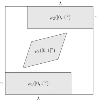
Example 3.3. We exhibit a dominated and strongly irreducible planar self-affine set X satisfying the strong separation condition and the projection condition. By Proposition 2.4 and Theorem 3.2, we thus have Cdim_A(X) = dim_A(X) = 1 + sup{dim_H(X∩(F+x)) :x∈X and F ∈X_F}.

ϕ₁([0,1]²)

ϕ₂([0,1]²)

ϕ3([0,1]²)

λ γ

λ

γ

Figure 1. Images of the unit square under the mappingsϕ_i in Example 3.3.

Fix

(i) 0< γ < ¹₂ < λ <1, (ii) a, b, d >0,

(iii) 0< v₃¹<1−a−b, (iv) γ < v₃² <1−γ−b−d, (v) ad > b², (vi) 1−2λ

1−2γ < a−d−p

(a−d)²+ 4b²

2b ,

and define

A1 = λ 0

0 γ

, A2 = λ 0

0 γ

, A3 = a b

b d

, and

ϕ₁(x, y) =A₁(x, y),

ϕ₂(x, y) =A₂(x, y) + (1−λ,1−γ), ϕ3(x, y) =A3(x, y) + (v₃¹, v₃²)

for all (x, y) ∈ R². Let X ⊂[0,1]² be the self-affine set associated to the tuple (ϕ₁, ϕ₂, ϕ₃); see Figure 1 for illustration.

Let us first show that the tupleA= (A1, A2, A3) is dominated and strongly irreducible. Since A₁ andA₂ preserve only the x-axis and y-axis and, by (ii),A₃ does not preserve neither axis nor their union, it follows thatAis strongly irreducible. By (v), the eigendirections of the symmetric matricesA₁,A₂, and A₃ corresponding to the largest eigenvalues in absolute value are

u₁ =u₂= (1,0) and u₃ =

a−d+p

(a−d)²+ 4b²

2b ,1

, respectively. Thus there existε >0 such that the closedε-neighborhood of

{span{tu₁+ (1−t)u₃} ∈RP¹ : 06t61}

gets mapped into its interior by all the matrices. Therefore,Ais dominated.

Let us then show thatX satisfies the strong separation condition and the projection condition.

The conditions (i)–(iv) guarantee that ϕi([0,1]²)∩ϕj([0,1]²) = ∅ whenever i6= j implying the

strong separation condition. To see that the projection condition holds, recall that, by the definition ofYF in (2.2),

[

i∈S

n∈N{1,2,3}ⁿ

A⁻¹_i Y_F ⊂ {span{(t,1)} ∈RP¹: a−d−p

(a−d)²+ 4b²

2b 6t60}.

Let Z be the self-affine set associated to the tuple (ϕ₁, ϕ₂). By (vi), it is enough to show that projspan{(t,1)}^⊥(Z) is a non-trivial closed line segment for all ^1−2λ_1−2γ < t 6 0. Up to a linear transformation, it is enough to show thatPt(Z) = [0,1−t] for all ^1−2λ_1−2γ < t60, where Pt(x, y) = x−ty for all (x, y)∈R². To see this, fix ^1−2λ_1−2γ < t60 and notice that it is sufficient to prove

Pt(ϕi([0,1]²)) = [

i∈{1,2}

Pt(ϕii([0,1]²)) (3.1) for all i∈S

n∈N{1,2}ⁿ. Indeed, if (3.1) holds, then P_t(Z) =P_t

^∞

\

n=1

[

i∈{1,2}ⁿ

ϕ_i([0,1]²)

=

∞

\

n=1

[

i∈{1,2}ⁿ

P_t(ϕ_i([0,1]²)) =P_t([0,1]²) = [0,1−t].

To prove (3.1), fix n∈N andi=i1· · ·in∈ {1,2}ⁿ. Write v1 = (0,0) andv2 = (1−λ,1−γ), and observe that

ϕ_i([0,1]²) =A_i([0,1]²) +ϕ_i(0) =Aⁿ₁([0,1]²) +

n

X

k=1

A_i|k−1v_in

= [0, λⁿ]×[0, γⁿ] + n

X

k=1

v_i¹

kλ^k−1,

n

X

k=1

v_i²

kγ^k−1

. Therefore,

Pt(ϕi([0,1]²)) =Pt

[0, λⁿ] +

n

X

k=1

v_i¹_kλ^k−1

×

[0, γⁿ] +

n

X

k=1

v²_ikγ^k−1

=

n

X

k=1

v_i¹_kλ^k−1−t

n

X

k=1

v_i²_kγ^k−1+ [0, λⁿ−tγⁿ].

Similarly, we see that

Pt(ϕi1([0,1]²)) =

n

X

k=1

v_i¹_kλ^k−1−t

n

X

k=1

v_i²_kγ^k−1+ [0, λⁿ⁺¹−tγⁿ⁺¹] and

Pt(ϕi2([0,1]²)) =

n

X

k=1

v_i¹_kλ^k−1+ (1−λ)λⁿ−t

n

X

k=1

v_i²_kγ^k−1−t(1−γ)γⁿ+ [0, λⁿ⁺¹−tγⁿ⁺¹].

Thus, P_t(ϕ_i([0,1]²)) = P_t(ϕ_i1([0,1]²))∪P_t(ϕ_i2([0,1]²)) if and only if (1−λ)λⁿ−t(1−γ)γⁿ 6 λⁿ⁺¹−tγⁿ⁺¹ or, equivalently, ^λ_γⁿn^(1−2λ)(1−2γ) 6t. Since ^1−2λ_1−2γ < t60, this holds for all n∈Nby (i).

4. Tangent sets

In this section, we develop the machinery to study the tangential structure of self-affine sets and prove Theorem 3.1. We begin with the following Poincar´e recurrence type lemma which allows us to approximate a given point (i, F) arbitrary well by the elements of the orbit of a generic point (j, L) under the dynamics introduced by the skew-product T: Σ×RP¹ →Σ×RP¹ defined in (2.4).

Lemma 4.1. Let A = (A₁, . . . , A_N) ∈ GL₂(R)^N and ν be a fully supported Bernoulli measure having simple Lyapunov spectrum. If µF is the Furstenberg measure with respect to ν, then there exists a set Θ⊂Σ×RP¹ with ν×µ_F(Θ) = 1 such thatϑ₁(j) exists,

χ₁(ν) =− lim

n→∞

1

nlogkA⁻¹_j|

n|ϑ₁(j)k⁻¹, χ2(ν) =− lim

n→∞

1

nlogkA⁻¹_j|

n|Lk⁻¹ for all(j, L)∈Θ, and there exists a countable dense set F so that

#{n∈N:Tⁿ(j, L)∈[i]×B(F,¹_k)}=∞ for all(j, L)∈Θ, i∈Σ∗, F ∈ F, and k∈N.

Proof. Since spt(µF) is a compact subset ofRP¹, such a countable dense setF ⊂spt(µF) exists.

Note thatν×µ_F([i]×B(F, r))>0 for alli∈Σ∗, F ∈ F, andr >0. The existence of the claimed set Θ⊂Σ×RP¹ now follows from Oseledets’ Theorem, Birkhoff Ergodic Theorem, and countability

of the parametersi∈Σ∗,F ∈ F, and k∈N.

Observe that the statement of Lemma 4.1 actually holds for everyF ∈spt(µF). We stated the lemma in the form we apply it later. We shall often use a lineL⊂R² to divide the plane into two half-planes (in the obvious way). In such situations we refer to these half-planes ashalf-planes determined byL.

Lemma 4.2. Let X be a planar self-affine set satisfying the strong separation condition and the projection condition. If ν is a fully supported Bernoulli measure, then the set

Bi ={F ∈RP¹:there exist k∈Σand n∈N such that πk∈F+πiand π[k|_n]is contained in one of the closed half-planes determined by F+πi} is at most countable for ν-almost alli∈Σ.

Proof. Let C = conv(X) be the convex hull of X and denote its interior by C^o. Let us first show that C^o∩X 6= ∅. Suppose to the contrary that C^o∩X = ∅. Then X ⊂ ∂C := C\C^o. By [24, Remark 3.4], we know thatX is not contained in a line and hence,∂C is not a line segment.

Let V ∈ S

n>n0

S

i∈ΣnA⁻¹_i YF. Since the projection condition holds, proj_V^⊥X is a non-trivial closed line segment and hence, there exist x1, x2 ∈∂C such thatx1−x2 ∈ V, the line segment connectingx₁ and x₂ is not contained in∂C, and x₁ ∈X orx₂∈X. Without loss of generality, we may assume that x₁ ∈X.

There are now two cases, eitherx2 ∈X or x2 ∈/ X. If x2 ∈/ X, then there exists an open arc J such that x₂ ∈J and J ⊂∂C\X, and whose endpoints w₁, w₂ ∈ R² are contained in X but w1−w₂ ∈/V. Since{x₁}=T

n∈Nϕi|_n(X) for somei∈Σ, there existsn∈Nsuch thatx1∈ϕi|_n(X) andV +x intersectsJ for allx∈ϕ_i|n(∂C)∩∂C. Observe thatϕ_i|n(X)⊂∂C is a self-affine set associated to the tuple (ϕ_i|n◦ϕ₁◦ϕ⁻¹_i|

n, . . . , ϕ_i|n◦ϕ_N ◦ϕ⁻¹_i|

n) and satisfies the strong separation condition. Thus,ϕ_i|n(X) cannot be a closed arc segment. Indeed, if ϕ_i|n(X) was a closed arc, then it is a union of closed arcs ϕ_i|n(ϕ_i(X)) which, by the strong separation condition, are pairwise disjoint, a contradiction. But this means that there exists an open arcI ⊂ϕ_i|n(∂C)∩∂C such thatX∩I = ∅, the endpoints v1, v2 ∈R² of I are in X and v1−v2 ∈/ V, and V +x intersects J for allx ∈ I. Thus, proj_V^⊥(X) ⊂ proj_V^⊥(∂C \(I ∪J)) = proj_V^⊥∂C \(proj_V^⊥I ∩proj_V^⊥J), where proj_V⊥I∩proj_V⊥J is clearly non-empty and open, and have both endpoints in proj_V⊥X contradicting the projection condition. Therefore,C^o∩X 6=∅provided that x2∈/ X.

If x₂ ∈ X, then, as {x₂} = T

m∈Nϕ_j|m(X) for some j ∈ Σ, there exists m ∈ N such that proj_V⊥ϕ_j|m(X)⊂(proj_V⊥X)^o andx₁∈/ ϕ_j|m(X). Againϕ_j|m(X) cannot be a closed arc and thus, there exists an open arcJ ⊂ϕ_j|m(∂C)∩∂C such thatJ∩X=∅ and the endpointsw1, w2 ∈R² of J are contained inX so thatw1−w2∈/ V. By the projection condition, for anyy∈J, V +y must