Working on strongly irreducible planar self-affine sets satis- fying the strong open set condition, we calculate the Birkhoff spectrum of continuous potentials and the Lyapunov spectrum

SELF-AFFINE SETS

BAL ´AZS B ´AR ´ANY, THOMAS JORDAN, ANTTI K ¨AENM ¨AKI, AND MICHA L RAMS

Abstract. Working on strongly irreducible planar self-affine sets satis- fying the strong open set condition, we calculate the Birkhoff spectrum of continuous potentials and the Lyapunov spectrum.

1. Introduction

Let Σ ={1, . . . , N}^Nbe the collection of all infinite words obtained from letters{1, . . . , N}, and let σ be the left-shift operator on Σ. The classical theorem of Birkhoff states that if µ is an ergodic σ-invariant probability measure, then ¹_nPn−1

k=0Φ(σ^ki) converges to the average R

ΣΦ dµ of Φ for every L¹ potential Φ : Σ → R^M and for µ-almost every i ∈ Σ. However, there are plenty of ergodicσ-invariant measures, for which the limit exists but converges to a different quantity. Furthermore, there are many words i∈Σ which are not generic for any ergodic measure or even for which the limit limn→∞ 1

n

Pn−1

k=0Φ(σ^ki) does not exist at all. Thus, one may ask how rich is the set of points

E_Φ(α) =n

i∈Σ : ¹_n

n−1

X

k=0

Φ(σ^ki)→α asn→ ∞o .

This ’richness’ is usually calculated in terms of topological entropy or Haus- dorff dimension. For a σ-invariant set A ⊂ Σ we denote the topological entropy ofσ on A by h_top(A) and the Hausdorff dimension of a setA⊂R^d by dimH(A). For the precise definitions, see Bowen [11] and Mattila [25].

The functions α 7→ h_top(E_Φ(α)) and α 7→ dim_H(E_Φ(α)) are respectively called the topological entropy spectrum and Hausdorff dimension spectrum of the Birfhoff averages of Φ. For simplicity they are also called the Birkhoff spectrum of Φ.

The topological entropy spectrum of Birkhoff averages has been intensely studied by several authors and is well understood for continuous potentials and vector valued continuous potentials; see Takens and Verbitskiy [29], Barreira, Saussol, and Schmeling [7] and Feng, Fan, and Wu [14], where [14]

considers the endpoints of the spectrum.

2010 Mathematics Subject Classification. Primary 28A80; Secondary 37L30, 37D35, 28D20.

Key words and phrases. Self-affine set, multifractal analysis, Birkhoff average, Lyapunov exponent, thermodynamic formalism.

1

In order to be able to study the Hausdorff dimension of the sets, where the limit of the Birkhoff average exists and takes a predefined value, we need to introduce a geometrical structure. The simplest example for such a geometrical structure is a self-similar iterated function system satisfying some separation condition.

Let fi:R^d→R^dbe contracting homeomorphisms fori∈ {1, . . . , N}. It is well known that there exists a non-empty, compact set X ⊂R^d such that X = S_N

i=1f_i(X). Moreover, there is a H¨older continuous map π: Σ → X, defined by π(i₁i₂· · ·) = limn→∞f_i1 ◦ · · · ◦f_in(0). If f_i(X)∩f_j(X) =∅ for i6= j, then the inverses of fi’s are well-defined. Therefore, π is invertible and its inverse is also H¨older continuous. Thus, the mapping T:X → X, T(π(i)) =π(σi), is well-defined, and one can study Hausdorff dimension of the sets

πE_Φ(α) =n

x∈X: lim

n→∞

1 n

n−1

X

k=0

Φ◦π⁻¹(T^k(x)) =αo .

Barreira and Saussol [6], Feng, Lau, and Wu [17], and Olsen [26] studied the setting where the f_i’s are conformal. In [6], the function Φ is H¨older continuous with codomain R, the paper [17] considers the case where Φ may be continuous and addresses the endpoints of the spectrum, and [26]

considers far more general Φ including the case where the codomain is R^d. In the conformal situation, a particular case of the Birkhoff averages, which is especially interesting from the dynamical systems’ theory point of view, is the Lyapunov spectrum, which is obtained by taking the potential i7→ −logkD_π(σi)fi|₁k. The Birkhoff average of this potential is called the Lyapunov exponent, and it is denoted by χ(i). The Lyapunov spectrum satisfies

dim_H(πEχ(α)) = htop(Eχ(α))

α ,

where E_χ(α) is the set of points i∈Σ for whichχ(i) =α.

The goal of this paper is to investigate the non-conformal situation. We consider the linear case, that is, the mappings fi are assumed to satisfy f_i(x) = A_ix+v_i, where v_i ∈ R^d and A_i ∈ GL_d(R) so that kA_ik < 1 for all i ∈ {1, . . . , N}. In this case, we have at the moment a very limited knowledge on the Hausdorff spectrum of Birkhoff averages. Barral and Mensi [4] studied the Birkhoff spectrum on Bedford-McMullen carpets. This result was generalised for Gatzouras-Lalley carpets by Reeve [28]. Moreover, Jordan and Simon [22] studied the case of planar affine iterated function systems with diagonal matrices for generic translation vectors vi. As far as we are aware of, the only known result about non-diagonal matrices comes from K¨aenm¨aki and Reeve [24], who investigated irreducible matrices with generic translation vectors (see Section 2 for the precise definition of irreducibility).

In the d-dimensional non-conformal situation, the Lyapunov exponents are in general not given by a Birkhoff average of some potential. However, under some domination conditions, it is still true. Barreira and Gelfert [5]

studied the topological entropy spectrum of the maximal Lyapunov exponent for non-linear, planar systems under certain domination condition, and Feng [15] studied it in the case of non-negative matrices in higher dimensions.

Later, Feng and Huang [16] calculated the topological entropy spectrum of maximal Lyapunov exponent in high generality. D´ıaz, Gelfert and Rams [13] investigated the non-dominated case for d = 2 providing results on topoligical entropy spectrum of the difference of the Lyapunov exponents and showing that the equality of Lyapunov exponents happens with positive but not maximal topological entropy for generic non-dominated systems.

In the main results of this paper, we calculate the Birkhoff and Lyapunov spectra for planar affine iterated function systems satisfying strong irreducibil- ity and the strong open set condition. After introducing some notation and preliminaries in Section 2.1, we formulate the results in Section 2.2. The key idea in the proof of the Birkhoff spectrum is to first calculate it on a family of affine iterated function systems which satisfy the dominated splitting condition. This is done in Section 4. The general case can then be approximated by systems satisfying the dominated splitting; see Section 5.

This idea, with suitable modifications, is also applied in the proof of the Lyapunov spectrum; see Section 6. Finally, we partially handle the boundary case in Section 7.

2. Main results

Throughout the rest of the paper, we restrict ourselves to planar systems.

2.1. Notation. A tuple Θ = (A1+v1, . . . , AN+vN) of contractive invertible affine self-maps on R² is called an affine iterated function system (affine IFS). The associated tuple of matrices (A1, . . . , AN) is therefore an element of GL₂(R)^N and satisfies maxi∈{1,...,N}kA_ik<1. As already mentioned in the introduction, there exists a unique non-empty compact setX⊂R² such that

X=

N

[

i=1

(Ai+vi)(X).

In this case, the set X is called a self-affine set. We say that Θ satisfies a strong open set condition (SOSC) if there exists an open set U ⊂ R² intersectingX such that the unionSN

i=1(Ai+vi)(U) is pairwise disjoint and is contained in U. Furthermore, Θ satisfies the strong separation condition (SSC) if (Ai+vi)(X)∩(Aj+vj)(X) =∅whenever i6=j.

We say that A = (A1, . . . , AN) ∈ GL2(R)^N is irreducible if there does not exist a 1-dimensional linear subspace V such that A_iV = V for all i∈ {1, . . . , N}; otherwiseAisreducible. The tupleAisstrongly irreducible if there does not exist a finite union of 1-dimensional subspaces,V, such that AiV =V for all i∈ {1, . . . , N}. In a reducible tupleA, all the matrices are simultaneously upper triangular in some basis. For tuples with more than one element, strong irreducibility is a generic property.

We say that A= (A1, . . . , AN) ∈GL2(R)^N is normalized if |det(Ai)|= 1 for i ∈ {1, . . . , N}. A matrix A is called hyperbolic if it has two real eigenvalues with different absolute value, elliptic if it has two complex eigenvalues, andparabolicif it is neither elliptic nor hyperbolic. The subgroup generated by Ais relatively compact if and only if the generated subgroup contains only elliptic matrices or orthogonal parabolic matrices. Otherwise we call it non-compact. For a hyperbolic matrixA, lets(A) be the eigenspace corresponding to the eigenvalue with the largest absolute value and let u(A) be the eigenspace corresponding to the smallest absolute valued eigenvalue.

Let Σ ={1, . . . , N}^Nbe the collection of all infinite words obtained from integers{1, . . . , N}. Ifi=i1i2· · · ∈Σ, then we define i|_n=i1· · ·in for all n∈N. The empty wordi|₀ is denoted by ∅. Define Σ_n={i|_n:i∈Σ} for alln∈N and Σ∗ =S

n∈NΣn∪ {∅}. Thus Σ_∗ is the collection of all finite words. The length of i∈Σ∗∪Σ is denoted by |i|. The longest common prefix ofi,j∈Σ∗∪Σ is denoted byi∧j. The concatenation of two words i∈Σ∗ and j∈Σ∗∪Σ is denoted by ij. Let σ be the left shift operator defined byσi=i₂i₃· · · for alli=i₁i₂· · · ∈Σ. If i∈Σ_nfor some n, then we set [i] ={j∈Σ :j|_n=i}. The set [i] is called acylinder set. The shift space Σ is compact in the topology generated by the cylinder sets. Moreover, the cylinder sets are open and closed in this topology and they generate the Borelσ-algebra.

WriteAi=Ai1· · ·Ain for all i=i1· · ·in∈Σn andn∈N. The canonical projection π: Σ → X is defined by π(i) = P∞

n=1A_i|n−1v_in for all i = i₁i₂· · · ∈Σ. It is easy to see thatπ(Σ) =X. If µis a measure on Σ, then we denote the pushforward measure of µunderπ byπ∗µ=µ◦π⁻¹.

LetM_σ(Σ) denote the collection of allσ-invariant probability measures on Σ andE_σ(Σ) be the collection of ergodic elements inM_σ(Σ). Letµ∈ M_σ(Σ) and recall that theKolmogorov-Sinai entropy of µand σ is

h(µ) :=h(µ, σ) =− lim

n→∞

1 n

X

i∈Σ_n

µ([i]) logµ([i]).

A probability measure µ on (Σ, σ) is Bernoulli if there exist a probability vector (p1, . . . , pN) such that

µ([i]) =p_i1· · ·p_in

for alli=i₁· · ·i_n∈Σ_nandn∈N. It is well-known that Bernoulli measures are ergodic. We say that µ ∈ M_σⁿ(Σ) is an n-step Bernoulli if it is a Bernoulli measure on (Σ, σⁿ). In this case, we write

˜ µ= _n¹

n−1

X

k=0

µ◦σ^−k (2.1)

and note that ˜µ∈ E_σ(Σ),h(µ, σⁿ) =nh(˜µ, σ), andR

ΣSnfdµ=nR

Σfd˜µfor all continuousf: Σ→R, whereS_nf =Pn−1

k=0f◦σ^k is theBirkhoff sum. In addition, if A= (A₁, . . . , A_N)∈GL₂(R)^N andµ∈ M_σ(Σ), then we define

theLyapunov exponents ofA with respect toµand σ to be χ1(µ) :=χ1(µ, σ) =− lim

n→∞

1 n

Z

Σ

logkA_i|nkdµ(i), χ₂(µ) :=χ₂(µ, σ) =− lim

n→∞

1 n

Z

Σ

logkA⁻¹_i|

nk⁻¹dµ(i).

(2.2)

We define a function χ:M_σ(Σ)→R² by settingχ(µ) = (χ₁(µ), χ₂(µ)) for all µ∈ M_σ(Σ). TheLyapunov exponents ati∈Σ are defined by

χ1(i) =−lim inf

n→∞

1

nlogkA_i|nk, χ₁(i) =−lim sup

n→∞

1

nlogkA_i|nk, χ₂(i) =−lim inf

n→∞

1

nlogkA⁻¹_i|

nk⁻¹, χ₂(i) =−lim sup

n→∞

1

nlogkA⁻¹_i|

nk⁻¹.

Ifχ_k(i) =χ_k(i), then we writeχk(i) for the common value. Recall that, by Kingman’s subadditive ergodic theorem, ifµ∈ E_σ(Σ), then (χ1(i), χ2(i)) = χ(µ) for µ-almost all i∈Σ. Since any two different ergodic measures are mutually singular, it is an interesting question to try to determine the size of a level set

Eχ(α) ={i∈Σ : (χ1(i), χ2(i)) =α}

for a given value α from the set P(χ) =

α∈R² :i∈Σ and (χ₁(i), χ₂(i)) =α . The Lyapunov dimension of µ∈ M_σ(Σ) is defined to be

dim_L(µ) = min h(µ)

χ₁(µ),1 +h(µ)−χ1(µ) χ₂(µ)

. We say that a potential ϕ: Σ∗ →[0,∞) is submultiplicative if

ϕ(ij)≤ϕ(i)ϕ(j)

for alli,j∈Σ∗. Recall that ifA∈GL₂(R), then the lengths of the semiaxes of the ellipse A(B(0,1)) are given by kAk and kA⁻¹k⁻¹. We define the singular value function with parameter sto be

ϕ^s(A) =







kAk^s, if 0≤s <1, kAkkA⁻¹k^−(s−1), if 1≤s <2,

|det(A)|^s/2, if 2≤s <∞.

Intuitively,ϕ^s(A) represents a measurement of the s-dimensional volume of the image of the unit ball underA. Sinceϕ^s(A) =|det(A)|^s−1kAk^2−sfor 1≤ s <2, we see that the functioni7→ϕ^s(A_i) defined on Σ∗ is submultiplicative.

By a slight abuse of notation, if the tuple (A₁, . . . , A_N)∈GL_d(R)^N is clear from the content, we refer to the function i7→ϕ^s(A_i) also byϕ^s.

We also need a more general class of potentials. Define ψ^q(i) =kA_ik^q1kA⁻¹_i k^−q2

for all q= (q1, q2)∈R². This is a generalisation of ϕ^s: by taking s⁰(s) =







(s,0), if 0≤s <1, (1, s−1), if 1≤s <2, (s/2, s/2), if 2≤s <∞,

(2.3)

it is easy to see that ψ^s0(s)=ϕ^s.

If Φ : Σ→Ris continuous, then we define the pressure by P(logϕ^s+ Φ) = lim

n→∞

1

nlog X

i∈Σ_n

ϕ^s(i) sup

j∈[i]

exp(S_nΦ(j)),

where the limit exists by subadditivity. For q= (q₁, q₂)∈R², one defines the pressure by

P(logψ^q) = lim

n→∞

1

nlog X

i∈Σn

ψ^q(i).

Note that if q1 ≥q2, thenψ^q is submultiplicative, and if q1 < q2, thenψ^q is supermultiplicative, which also guarantees the existence of the limit.

Given a continuous potential Φ : Σ→R^M, we let P(Φ) ={α∈R^M :i∈Σ and lim

n→∞

1

nS_nΦ(i) =α}

={α∈R^M :µ∈ M_σ(Σ) and Z

Σ

Φ dµ=α}

be the set of possible values of Birkhoff averages. Note that the equality above follows from [27, Theorem 2.1.6 and Remark 2.1.15]. Write

E_Φ(α) ={i∈Σ : lim

n→∞

1

nS_nΦ(i) =α}

for all α∈R^M.

We use Bowen’s definition [11] of topological entropy which is defined for non-compact and non-invariant sets. It follows from Takens and Verbitskiy [29, Theorem 5.1] that

h_top(E_Φ(α)) = lim

ε↓0lim inf

n→∞

1

nlog #{i|_n∈Σ_n:|α−_n¹S_nΦ(i)|< ε}, (2.4) where | · | denotes the Euclidean norm in R^M. Note that the result is for continuous potentials having range in R but it easily extends to the case where the range is in R^M. Recall that, by Bowen [11], we have

h_top(E)≥sup{h(µ) :µ∈ M_σ(Σ) and µ(E) = 1}.

The topological closure of a setA is denoted byA, the boundary by∂A, and the interior by A^o.

2.2. Main theorems. We are now ready to formulate our main theorems.

The results determine the Hausdorff dimensions of the canonical projections of EΦ(α) andEχ(α).

Theorem 2.1 (Birkhoff spectrum). Let (A₁+v₁, . . . , A_N+v_N) be an affine IFS on R² satisfying the SOSC andΦ : Σ→R^M be a continuous potential.

If (A₁, . . . , A_N)∈ GL₂(R)^N is strongly irreducible such that the generated subgroup of the normalized matrices is not relatively compact, then P(Φ)is compact and convex, and

dimH(πEΦ(α)) = sup{dim_L(µ) :µ∈ M_σ(Σ)and Z

Σ

Φ dµ=α}

= sup{dim_L(µ) :µ∈ E_σ(Σ)and Z

Σ

Φ dµ=α}

= sup{s≥0 : inf

q∈R^M

P(logϕ^s+hq,Φ−αi)≥0}

for all α∈ P(Φ)^o⊂R^M. Furthermore, the function α7→dim_H(πE_Φ(α)) is continuous on P(Φ)^o.

Theorem 2.2 (Lyapunov spectrum). Let (A1 +v1, . . . , A_N +v_N) be an affine IFS onR² satisfying the SOSC. If(A1, . . . , AN)∈GL2(R)^N is strongly irreducible such that the generated subgroup of the normalized matrices is not relatively compact, then

dim_H(πE_χ(α)) = sup{dim_L(µ) :µ∈ M_σ(Σ) andχ(µ) =α}

= sup{dim_L(µ) :µ∈ E_σ(Σ) andχ(µ) =α}

= sup{s≥0 : inf

q∈R²

{P(logψ^s0(s)−q)− hq, αi} ≥0}

= min

h_top(E_χ(α)) α1

,1 +h_top(E_χ(α))−α₁ α2

for all α = (α1, α2) ∈ P(χ)^o ⊂R², where s⁰:R+ → R² is defined in (2.3).

Furthermore, if α∈ P(χ)∩ {(α₁, α₂)∈R² :α₁ =α₂}, then dim_H(πE_χ(α)) = lim

ε↓0sup{dim_L(µ) :µ∈ M_σ(Σ)and |χ(µ)−α| ≤ε}.

Moreover,P(χ) is convex and compact, and the functionα7→dimH(πEχ(α)) is continuous onP(χ)^o∪(P(χ)∩ {(α₁, α₂)∈R² :α₁=α₂}).

2.3. Further discussion. If the generated subgroup of the normalised ma- trices is compact, then we haveχ₁(µ) =χ₂(µ) for any invariant measureµ.

Therefore, Theorem 2.1 is still true in this setting, but rather than following the proof in this paper, it is a simpler approach to use the standard conformal methods. Furthermore, it seems possible to discard the SOSC and consider the overlapping case; see Remark 4.5.

In the conformal setting, both the Lyapunov spectrum and the Birkhoff spectrum have a unique maximum which corresponds to the integral of the measure of maximal dimension. The non-conformal case is more involved.

For the Birkhoff spectrum, in the setting of Theorem 2.1, it is possible to show that there will be at most one maximum. If we let s = dim_H(X) and µ be the unique ergodic measure with Lyapunov dimension s then for any α ∈ P(Φ)^o ⊂ R^M, dim_H(πE_Φ(α)) = s if and only if R

ΣΦ dµ = α.

To see this first note that if α ∈ P(Φ)^o ⊂ R^M and R

ΣΦ dµ = α then dimH(πEΦ(α)) = s is an immediate consequence of Theorem 2.1. On the other hand, if dim_H(πE_Φ(α)) =sthen there exists a sequence of invariant measures µn with R

ΣΦ dµn =α for eachn∈N and limn→∞dimL(µn) =s.

Any weak^∗ limit of these measures must be invariant and have integral α.

By K¨aenm¨aki and Reeve [24, Proposition 6.8], it follows that the Lyapunov dimension must be at least s, and so the weak^∗ limit must be the unique measure of maximal Lyapunov dimensionµ andR

ΣΦ dµ=α.

In Theorem 2.1, in the case where the self-affine system is dominated and the function Φ is H¨older, it is possible to show that the spectrum varies analytically away from integer values. The argument would follow the one given in Barreira and Saussol [6] with an adaptation for the case of higher dimensions. The same argument also holds in Theorem 2.2 when the system is dominated.

In the situation, where the system is not strongly irreducible, the results are no longer always true; for example, see Reeve [28] where the author considers self-affine carpets. In the diagonal case, it would be possible to combine Hochman [20] and Jordan and Simon [22] to get results for a large class of systems based on the dimension of projections of measures onto the x-axis and y-axis.

In addition to the obtained results it is possible to adapt our methods to obtain analogous results for sets with a similar definition toE_χ(α). For example, under the same assumptions as for Theorem 2.2, the sets

Eχ,s(α) ={i∈Σ : lim

n→∞

1

nlogϕ^s(i) =α}

could be considered for s >0. The method would be very similar to first show the results for dominated system and then deduce the full result by a slight adpatation of Lemma 5.4. This approach would also work for the sets

Eχ(α) ={i∈Σ :χ2(i) =α}.

Lemma 5.4 also gives a simple proof for the continuity of the pressure P with respect to the matrix tuples in the two-dimensional case; see Feng and Shmerkin [18]. Namely, P is upper semicontinuous since, by definition, it is an infimum of continuous functions. Lemma 5.4 implies that it is a supremum of continuous functions, so it is also lower semicontinuous and hence continuous.

In Theorem 2.1, if P(Φ) has empty interior, then it means that P(Φ) will be contained in somek-dimensional hyperplane where k < m. If P(Φ) has nonempty interior in this hyperplane then our results still apply. In Theorem 2.2, if P(χ) has empty interior, then, since it is a convex set, it is either contained in a one dimensional hyperplane or a point. In the case, where it

is a one-dimensional hyperplane again we can work with the interior when restricted to this line. The proofs for these cases are virtually identical to the given ones, hence, we omit them.

As an important part of the study of the Birkhoff averages, one is also interested in the set

D_Φ=n

i∈Σ : lim

n→∞

1 n

n−1

X

k=0

Φ(σ^ki) does not existo .

In the conformal case, it holds that dimH(πDΦ) = dimH(X); see Barreira and Schmeling [8]. It would be interesting to see if the same holds also in our setting. The lower bounds we obtain rely on finding the dimension of Bernoulli measures, which cannot help for this question. The same problem appears also in the question whether dimH(πGµ) = dimL(µ), where

Gµ= n

i∈Σ : _n¹

n−1

X

k=0

δ_σki converges weakly to µ o

for all µ∈ M_σ(Σ).

For shift spaces the topological entropy spectrum for Birkhoff averages of a continuous function is concave and can be written as a Legendre transform of a suitable pressure function, see Takens and Verbitskiy [29, Section 6]. For an expanding interval Markov map the Lyapunov spectrum is a simple transform of the topological entropy spectrum for a suitable potential. This means that the Lyapunov spectrum in this setting is a straightforward transform of a concave function (however the transform does not necessary preserve the concavity). In the setting of Theorem 2.2, the function α7→h_top(E_ξ(α)) will still be concave (see Proposition 7.6) and so the Lyapunov spectrum is again a transform of a concave function but again it will not necessarily preserve concavity. It should be possible by careful case by case analysis to determine certain regions for which the Birkhoff spectrum and Lyapunov spectrum are concave but in general they will not be concave.

Finally, it is a natural question to ask whether the results could be extended to higher dimensions. There are two stumbling blocks to this. Firstly the result on the dimension of Bernoulli measures for strongly irreducible systems in B´ar´any, Hochman, and Rapaport [2] is only proved in the dimension two (see Hochman and Rapaport [21, Section 1.6] for discussion). Also the approximation via dominated systems becomes much more problematic in higher dimensions.

3. Upper bound

Throughout the paper, our only assumption about the potential Φ is that it is continuous. A standard lemma gives bounds on the variation of SnΦ insidenth level cylinders.

Lemma 3.1. For any continuous Φ : Σ→R^M,

n→∞lim

1 nmax

k∈Σn

i,j∈[k]max |S_nΦ(i)−SnΦ(j)|= 0.

Proof. Denote by Varn(Φ) the nth variation of the potential Φ, i.e.

Var_n(Φ) = max

k∈Σ_n max

i,j∈[k]|Φ(i)−Φ(j)|.

By the compactness of Σ, we have Varn(Φ)→0. The assertion follows since

1 nmax

k∈Σn

i,j∈[k]max |S_nΦ(i)−S_nΦ(j)| ≤ _n¹

n

X

k=1

Var_k(Φ)

for all n∈N.

The next proposition gives an upper bound for the dimension of πE_Φ(α) by means of the pressure. Its proof is a standard covering argument.

Proposition 3.2. Let (A1+v1, . . . , A_N+v_N) be an affine IFS on R² and Φ : Σ→R^M be a continuous potential. Then

dimH(πEΦ(α))≤sup{s≥0 : inf

q∈R^M

P(logϕ^s+hq,Φ−αi)≥0}

for all α∈ P(Φ)^o. Proof. Observe that

EΦ(α)⊂

∞

\

r=1

∞

[

n=1

∞

\

m=n

[

i∈Dm,r

[i], where

D_m,r ={i∈Σ_m :j∈[i] and|_m¹S_mΦ(j)−α|< ¹_r}.

By Lemma 3.1, there exists ζ > 0 such that |_m¹SmΦ(j)−α| < ²_r for all m≥ −logζ,i∈Σ_m, and j∈[i]. Therefore,

−2m|q|

r ≤ hq, S_mΦ(j)−mαi ≤ sup

j∈[i]

hq, S_mΦ(j)−mαi (3.1) for all i∈Dm,r and m≥ −logζ.

Let s₀(α) = sup{s≥0 : inf_q∈RM P(logϕ^s+hq,Φ−αi) ≥0} and choose s > s₀(α). Thus there existsq =q(α, s) such thatP(logϕ^s+hq,Φ−αi)<0.

Write P =P(logϕ^s+hq,Φ−αi) and letγ >0 be such that X

i∈Σm

ϕ^s(i) exp( sup

j∈[i]

hq, S_mΦ(j)−mαi)< e^{mP /2} (3.2) for all m≥ −logγ. AskA_ik ≤λ^|i|for someλ <1, we have

ϕ^s+c(i)≤ϕ^s(i)e^c|i|logλ (3.3)

for all c≥ 0. Hence, for every δ < min{γ, ζ}, we have by (3.3), (3.1) and (3.2)

H^s−2|q|/r_δ ^logλ(πE_Φ(α))≤

∞

X

m=d−logδe

X

i∈D_m,r

ϕ^{s−2|q|/rlogλ}(i)

≤

∞

X

m=d−logδe

X

i∈D_m,r

ϕ^s(i)e^−2m|q|/r

≤

∞

X

m=d−logδe

X

i∈Dm,r

ϕ^s(i) exp( sup

j∈[i]

hq, S_mΦ(j)−mαi)

≤

∞

X

m=d−logδe

e^{mP /2}.

By letting δ↓0, the upper bound above approaches to zero and hence, by letting r→ ∞, dim_H(πEΦ(α))≤s. The proof is finished as s > s0(α) was

arbitrary.

4. Birkhoff averages

We let RP¹ denote the real projective line, which is the set of all lines through the origin in R². We call a proper subsetC ⊂RP¹ a cone if it is a closed projective interval and a multicone if it is a finite union of cones. Let A = (A1, . . . , AN) ∈GL2(R)^N. We say that A is dominated if there exists a multicone C ⊂ RP¹ such that SN

i=1AiC ⊂ C^o. By [9, Theorem B], A is dominated if and only if there exist constantsC >0 and 0< τ <1 such that

|det(A_i)|

kA_ik² ≤Cτⁿ

for all i ∈ Σn and n ∈ N. Furthermore, if A is dominated, then, by [3, Lemma 2.4], the mappingV: Σ→RP¹ defined by

V(i) =

∞

\

k=0

Ai|_kC (4.1)

is H¨older continuous.

Proposition 4.1. If (A1, . . . , A_N) ∈ GL2(R)^N is dominated, then there existsC >0 such that

kA_i|V(σⁿi)k ≥CkA_ik

for all i∈Σn and n∈N. In particular, the function i7→logkA_i|1|V(σi)k is H¨older continuous and

|logkA_i|nk −SnlogkA_i|1|V(σi)k| ≤C for all i∈Σ and n∈N.

Proof. This follows from Bochi and Morris [10, Lemma 2.2] and B´ar´any and

Rams [3, Lemma 2.4].

If (A1. . . , AN)∈GL2(R)^Nis dominated, then we define Ψ = (Ψ1,Ψ2) : Σ→ R² by setting

Ψ1(i) =−logkA_i|1|V(σi)k,

Ψ₂(i) =−log|det(A_i|1)|+ logkA_i|1|V(σi)k, (4.2) for alli∈Σ. Proposition 4.1 implies that Ψ is a H¨older continuous potential

and Z

Σ

Ψ dµ=χ(µ)

for all µ∈ M_σ(Σ), where χis defined in (2.2). We also define Ψ^s(i) =







−sΨ₁(i), if 0≤s <1,

−Ψ₁(i)−(s−1)Ψ2(i), if 1≤s <2,

−s(Ψ₁(i) + Ψ2(i))/2, if 2≤s <∞, for all i∈Σ.

Given a potential Φ : Σ→R^M, we wish to find, for anyα ∈ P(Φ)^o, a fully supported n-step Bernoulli measure ν with Birkhoff average R

ΣΦ dν =α and with large Lyapunov dimension. We will use Proposition 4.1 to find such measures with Birkhoff average close to α, but to find the exact match we will need the following technical lemma which is along the lines of Hopf’s Lemma.

Lemma 4.2. Let f:R^M → (0,∞) be a C¹ convex function and g = ∇f.

For a >0 letQ={x∈R^M :f(x)≤a}. If Q is bounded and nonempty such that|g(x)|> b >0 for all x∈∂Q, then B(0, b)⊂g(Q).

Proof. Qis convex and∂Qis a smooth manifold. For anyx∈∂Q,g(x)/|g(x)|

is the outer normal to ∂Qat x. As we can perturb Qslightly to obtain a strictly convex set, we can find a (positively oriented) bijectionn:S^M−1 →

∂Q such that n⁻¹(x) is an outer vector at every x ∈ ∂Q. The map ` = g◦n/|g◦n| maps S<sup>M−1</sup> into itself and satisfies hy, `(y)i ≥ 0, hence ` is homotopic to the identity (the homotopy is given by h(y, γ) = (γy+ (1− γ)`(y))/|γy + (1−γ)`(y)|). This implies that the topological degree is deg(g, Q,0) = deg(`, S^M−1,0) = 1.

As g(x)≥b for all x∈∂Q, for everyr ∈R^M,|r|< b,g is homotopic to g−r rel 0 on ∂Q. Thus, deg(g, Q, r) = deg(g−r, Q,0) = deg(g, Q,0) = 1.

Since this impliesB(0, b)⊂g(Q), we are done.

Proposition 4.3. Let A = (A₁, . . . , A_N) ∈ GL₂(R)^N be dominated and Φ : Σ→R^M be a continuous potential. If α∈ P(Φ)^o, then for every

s <sup{s≥0 : inf

q∈R^M

P(logϕ^s+hq,Φ−αi)≥0}

there exists a fully supportedn-step Bernoulli measureν such thatdim_L(ν) = dim_L(˜ν)≥sand R

ΣΦ d˜ν =α, where ˜ν is defined in (2.1).

Proof. Let s < sup{s ≥ 0 : inf_q∈R^MP(logϕ^s+hq,Φ−αi) ≥ 0} and note that, by Proposition 4.1, we have

P(logϕ^s+hq,Φ−αi) =P(Ψ^s+hq,Φ−αi).

Since for any q∈R^m s→P(Ψ^s+hq,Φ−αi) is strictly decreasing we have that

inf{P(Ψ^s+hq,Φ−αi) :q ∈R^M}>0.

Since α∈ P(Φ)^o we can find η >0 such that for any q ∈R^M with |q|= 1 we can find an invariant measureµ such thatR

Φ dµ−α=ηq. Therefore by the variational principle for any q∈R^m

P(Ψ^s+hq,Φ−αi)≥h(µ) + Z

log Φ^sdµ+η|q|

whereh(µ)+R

log Φ^sdµis bounded uniformly below for all invariant measures.

Thus for

δ= inf{P(Ψ^s+hq,Φ−αi) :q ∈R^M}>0 we can chooseq0>0 so that

P(Ψ^s+hq,Φ−αi)≥3δ whenever |q| ≥q₀. We fix ε₁, ε₂ >0 such that

ε₁q₀+ε₂< δ/4.

Since Φ and Ψ^s are continuous, we can, by Lemma 3.1, choosen∈Nsuch that

i∈Σmaxn

j,k∈[i]max{|S_nΦ(j)−SnΦ(k)|} ≤nε1

and

i∈Σmaxn

j,k∈[i]max{|S_nΨ^s(j)−SnΨ^s(k)|} ≤nε2.

Therefore, we can find functions Φn and Ψn which are constant onnth level cylinders and where

kS_nΦ−Φ_nk_∞≤nε₁ and kS_nΨ^s−Ψ_nk_∞≤nε₂.

We now work with the pressure for σⁿwhich we denote byPn. Note that we have P_n(S_n·) =nP(·). Thus we have

inf{P_n(S_nΨ^s+hq, S_nΦ−nαi) :|q| ≤q₀}=nδ and

inf{P_n(SnΨ^s+hq, S_nΦ−nαi) :|q|=q0} ≥3nδ.

Since ε₁|q₀|+ε₂< δ/4, we see that

min{P_n(Ψn+hq,Φn−nαi) :|q| ≤q0} ∈ 3nδ

4 ,5nδ 4

(4.3) and

min{P_n(Ψ_n+hq,Φ_n−nαi) :|q|=q₀} ≥ 11nδ 4 .

Since Φn and Ψn are locally constant, and therefore H¨older continuous, the functionq 7→P_n(Ψ_n+hq,Φ_n−nαi) is analytic and convex. Moreover, for any q∗ ∈R^M we have

∇ _q=q

∗Pn(Ψn+hq,Φn−nαi) = Z

Σ

(Φn−nα) dµq∗,

where µq∗ is the equilibrium state for Ψn+hq_∗,Φn−nαi. Note that the set Q={q :P_n(Ψ_n+hq,Φ_n−nαi)≤2nδ} ⊂B(0, q₀)

is convex. By convexity and (4.3), we get

|∇P_n(Ψn+hq,Φn−nαi)|

≥ Pn(Ψn+hq,Φn−nαi)−Pn(Ψn+hq,˜ Φn−nαi)

|q−q|˜ ≥ 3nδ

8q₀ for all q∈∂Q.

Define f1, f2:Q→R^M by setting f1(q) =

Z

Σ

(Φn−nα) dµq=∇P_n(Ψn+hq,Φn−nαi) and

f2(q) = Z

Σ

(SnΦ−nα) dµq. By Lemma 4.2,f1(Q)⊃B(0,^3nδ_8q

0). Since kf₁−f2k_∞≤ε1n < 3nδ

8q₀, we have

|(1−t)f1(q) +tf2(q)| ≥ 3δn 8q0

−t|f₁(q)−f2(q)| ≥ 3δn 8q0

−ε1n >0 for allt∈[0,1] andq ∈∂Q. It follows thatf1|_∂Q andf2|_∂Q are homotopic onR^M \ {0} and hence 0∈f2(Q). This means that there exists q1∈Qsuch thatR

ΣS_nΦ dµ_q1 =nα. Now, by (4.3), 3nδ

4 ≤Pn(Ψn+hq₁,Φn−nαi)

=h(µq1, σⁿ) + Z

Σ

Ψn+hq₁,Φn−nαidµq1. So

h(µq1, σⁿ) +nδ 4 +

Z

Σ

SnΨ^sdµq1 ≥ 3nδ 4 and

h(µ_q1, σⁿ) + Z

Σ

S_nΨ^sdµ_q1 ≥0.

If 0≤s <1, then we have

dim_L(µ_q1) = h(µ_q1, σⁿ)

χ1(µq1, σⁿ) = h(µ_q1, σⁿ) R

ΣSnΨ1dµq1

≥s.

Alternatively, if 1≤s <2, then

h(µq1, σⁿ) +χ1(µq1, σⁿ) + (s−1)χ2(µq1, σⁿ)≥0 and rearranging gives that

dimL(µq1) = 1 +h(µ_q1, σⁿ)−χ₁(µ_q1, σⁿ) χ2(µq1, σⁿ) ≥s.

The case s ≥2 is left to the reader. Since µ_q1 is an equilibrium state for Ψ_n+hq₁,Φ_n−nαi, which is constant onnth level cylinders, it is aσⁿ-invariant Bernoulli measure. Takingν =µq1 finishes the proof.

We remind the reader that the (lower) Hausdorff dimension of the measure µon R² is defined by

dim_H(µ) = inf{dim_H(A) :µ(A)>0}.

In order to provide the lower bounds in the main theorems, we find invariant measures with prescribed integrals and Lyapunov exponents, for which we can calculate the Hausdorff dimension. The following theorem guarantees thatn-step Bernoulli measures can be used for this purpose.

Theorem 4.4. Let(A1+v1, . . . , AN+vN)be an affine IFS onR² satisfying the SOSC. If (A₁, . . . , A_N)∈GL₂(R)^N is strongly irreducible such that the generated subgroup of the normalized matrices is non-compact, then

dimH(π∗µ) = dimL(µ) for all Bernoulli measures µ onΣ.

Proof. This is by B´ar´any, Hochman, and Rapaport [2, Theorem 1.2].

Remark 4.5. In a very recent preprint of Hochman and Rapaport [21] the above result has been generalized to a case which allows severe overlapping.

The strong open set condition has been replaced by the assumption that the defining affine maps do not share a fixed point and are exponentially separated; see [21, Theorem 1.1]. Relying on this, instead of Theorem 4.4, would improve our main results accordingly.

We are now able to prove Theorem 2.1 for dominated systems.

Theorem 4.6. Let(A1+v1, . . . , A_N+v_N)be an affine IFS onR² satisfying the SOSC and Φ : Σ → R^M be a continuous potential. If (A1, . . . , AN) ∈ GL₂(R)^N is strongly irreducible and dominated such that the generated subgroup of the normalized matrices is non-compact, then

dim_H(πE_Φ(α)) = sup{dim_L(µ) :µ∈ M_σ(Σ)and Z

Σ

Φ dµ=α}

= sup{s≥0 : inf

q∈R^M

P(logϕ^s+hq,Φ−αi)≥0}

for all α∈ P(Φ)^o.

Proof. It follows from Propositions 3.2 and 4.3 that dimH(πEΦ(α))≤sup{s≥0 : inf

q∈R^M

P(logϕ^s+hq,Φ−αi)≥0}

≤sup{dim_L(˜ν) :ν is fully supportedn-step Bernoulli and

Z

Σ

Φ d˜ν =α}

≤sup{dim_L(µ) :µ∈ M_σ(Σ) and Z

Σ

Φ dµ=α}, where ˜ν is defined in (2.1). Let µ∈ M_σ(Σ) be such thatR

ΣΦ dµ=α. By the variational principle (see [12, 23]), if s <dim_L(µ), then

P(logϕ^s+hq,Φ−αi)≥h(µ) + lim

n→∞

1 n

Z

Σ

logϕ^s(A_i|n) dµ(i)>0 for all q∈R^M. Therefore,s≤sup{s≥0 : inf_q∈RM P(logϕ^s+hq,Φ−αi)≥ 0} and, consequently,

sup{dim_L(µ) :µ∈ M_σ(Σ) and Z

Σ

Φ dµ=α}

≤sup{s≥0 : inf

q∈R^M

P(logϕ^s+hq,Φ−αi)≥0}.

Finally, letν be a fully supportedn-step Bernoulli measure so thatR

ΣΦ d˜ν = α. Then clearly ˜ν(E_Φ(α)) = 1 and, by Theorem 4.4,

dimL(˜ν) = dimH(π∗ν)˜ ≤dimH(πEΦ(α))

finishing the proof.

5. Dominated subsystems

We begin the section with the proof of a key lemma in order to construct dominated subsystems.

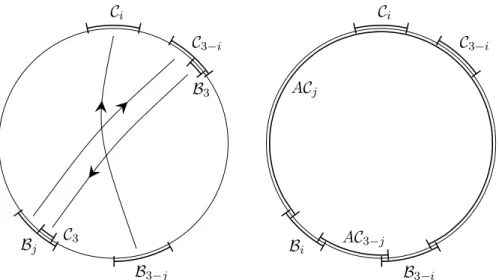
Lemma 5.1. LetA₁, A₂, A₃ ∈GL₂(R) such that there exist conesB₁,B₂,B₃ and C₁,C₂,C₃ such that

(1) B₁∩ B₂ =∅, C₁∩ C₂=∅, C₁∩ B₁ =∅, and C₂∩ B₂=∅, (2) there existi₁, j₁ ∈ {1,2} such that C₃ ⊂ B_i^o

1 and B₃⊂ C_j^o

1, (3) Ai(RP¹\ B_i)⊂ C_i^o for everyi∈ {1,2,3}.

We then have that for every A∈GL2(R) which is hyperbolic withu(A)∈ C_i^o and s(A) ∈ B_j^o there exist i, j ∈ {1,2} such that AiA3AA²_j(C₁ ∪ C₂) ⊂ (C₁∪ C₂)^o. For every other A ∈ GL₂(R) there exist i, j ∈ {1,2} such that

A²_iAA²_j(C₁∪ C₂)⊂(C₁∪ C₂)^o.

Proof. First, let us make a couple of remarks. It is easy to see thatAi(C₁∪ C₂)⊂ C_i^o for i∈ {1,2}. This means that A3−i1C₃ ⊂ C_3−i^o

1. Finally, we note that if a coneC satisfies C ∩(C₁∪ C₂) =∅, thenA₃C ⊂ C₃^o.

FixA∈GL2(R). We see that there are two possible cases:

(1) there existi, j∈ {1,2} such thatAC_j ∩ B^o_i =∅,

C_i

C_3−i

C₃ B_j

B_3−j B₃

C_i

C_3−i

B_i

B_3−i AC_3−j AC_j

Figure 1. The left-hand side image illustrates the assump- tions in Lemma 5.1 and the image on the right depicts one of the possible situations in the case (2) of the proof.

(2) for every i, j∈ {1,2} we have AC_i∩ B^o_j 6=∅.

In the case (1), since AC_j∩ B_i^o =∅, we have A_i(AC_j)⊂A_i(RP¹\ B_i)⊂ C_i^o. Thus,

A²_iAA²_j(C₁∪ C₂)⊂A²_iAC_j^o⊂ C_i^o ⊂(C₁∪ C₂)^o.

On the other hand, if the case (2) holds, then A(RP¹\(C₁∪ C₂)) ⊂ B₁^o∪ B^o₂. Since B₁ and B₂ are disjoint intervals on RP¹, one of the connected components of (RP¹\(C₁∪ C₂)) is contained in B^o₁, and the other one is contained in B^o₂. In particular, there are k, k⁰ ∈ {1,2} so that AB₁ ⊂ B_k^o and AB₂ ⊂ B_k^o0. Now, if k 6= k⁰ then A²B₁ ⊂ B^o₁ and A²B₂ ⊂ B^o₂, which is a contradiction, since it would imply that A² has two different stable eigenspaces. Similar argument can be applied for the conesC₁ andC₂, and the inverse matrix A⁻¹.

Thus, there exist unique i, j∈ {1,2}such that AB_i⊂ B_i^o andA⁻¹C_j ⊂ C_j^o. Thus, in particular, A is a hyperbolic matrix with stable and unstable eigenspacess(A)∈ B^o_i and u(A)∈ C_j^o. Moreover,AC_3−j∩(C₁∪ C₂) =∅; see Figure 1. Thus,

A3−i1A₃AA²_3−j(C₁∪ C₂)⊂A3−i1A₃AC_3−j^o ⊂A3−i1C₃^o ⊂ C_3−i^o

1 ⊂(C₁∪ C₂)^o

and the proof is finished.

Lemma 5.2. Let (A₁, . . . , A_N)∈GL₂(R)^N be strongly irreducible such that the generated subgroup of the normalized matrices is non-compact. Then

there existK ∈N and multicones B and C such that B ⊂ C^o, and for every i∈Σ∗ there exist j₁,j₂∈Σ_K such that

Aj1AiAj2C ⊂ B^o.

Proof. Since the tuple is strongly irreducible and the generated subgroup of the normalized matrices is non-compact, there existk1,k2 ∈Σ∗ such that Ak1 andAk2 are hyperbolic and the spacess(Ak1), s(Ak2), u(Ak1), u(Ak2) are all different. By taking powers, one can choose k1 andk2 so that|k1|=|k2|.

Letr >0 be so small such that

B(s(A_k1), r)∩B(s(A_k2), r) =B(u(A_k1), r)∩B(u(A_k2), r)

=B(s(Aki), r)∩B(u(Akj), r) =∅, (5.1) where B(x, r) denotes the closed ball centered at x and with radiusr. Thus, there existsL=L(r)≥1 such that

(Aki)^L(RP¹\B(u(Aki), r))⊂B(s(Aki), r)^o fori∈ {1,2}. We distinguish two cases:

(1) there exists r > 0 such that u(A_i) ∈/ B(s(A_ki), r) or s(A_i) ∈/ B(u(Aki), r) for all i∈Σ∗ and i∈ {1,2},

(2) for every r >0 there exists i∈ Σ∗ such thatu(A_i)∈ B(s(A_ki), r) ands(Ai)∈B(u(Akj), r) for some i, j∈ {1,2}.

In the case (1), by Lemma 5.1, we see that for every i ∈ Σ∗ there exist i, j∈ {1,2} so that

(A_ki)^2LA_i(A_kj)^2L(B(s(A_k1), r)∪B(s(A_k2), r))

⊂(B(s(A_k1), r)∪B(s(A_k2), r))^o.

If the case (2) holds, then fix r > 0 so that (5.1) holds. Let k3 be such that u(A_k3) ∈ B(s(A_ki), r) and s(A_k3) ∈B(u(A_kj), r). By choosing ρ >0 sufficently small, we have B(u(Ak3), ρ) ⊂B(s(Aki), r) and B(s(Ak3), ρ) ⊂ B(u(A_kj), r). Therefore, by choosingM ∈Nsufficiently large, we have

(Ak3)^M(RP¹\B(u(Aki), ρ))⊂B(s(Aki), ρ)^o.

By taking powers, we can assume that M|k3| = |k1| = |k2|. Thus, the statement of the lemma again follows by applying Lemma 5.1, with K = 2Lmax|k₁|and C=B(s(A_k1), r)∪B(s(A_k2), r).

By Lemma 5.2, there exists K ≥ 1 such that for every n > 2K and i∈Σn−2K there exist j1 =j1(i) andj2 =j2(i) such that the tuple

(A_k)_k∈Σ^D

n, where Σ^D_n ={j₁(i)ij₂(i) :i∈Σn−2K}, (5.2) is dominated and strongly irreducible. Note that Σ^D_n ⊂Σn for alln >2K. If n >2K and ϕ: Σ→Ris a subadditive potential, then we define a pressure on the dominated subsystem by setting

PD,n(logϕ) = lim

k→∞

1

klog X

i1,...,ik∈Σ^D_n

ϕ(i1· · ·ik).

Note that the condition given by Lemma 5.2 is stronger than the usual domination, see Avila, Bochi, and Yoccoz [1] and Bochi and Gourmelon [9].

In particular, we have the following uniform bound.

Lemma 5.3. Let multiconesB andC be such thatB ⊂ C^o. Then there exists Z >0 such that for every pair of matricesA andB satisfyingAC ∪BC ⊂ B^o we have

kABk ≥e^−ZkAkkBk.

Proof. This follows easily from Bochi and Morris [10, Lemma 2.2].

The lemma guarantees that in every subsemigroup of S

n∈NΣ^D_n the norm (and hence alsoϕ^sfor alls∈[0,∞)) is almost multiplicative up to a uniformly

chosen constant.

Lemma 5.4. Let Φ : Σ→R^M be a continuous potential. Then

n→∞lim

1

nPD,n(logϕ^s+hq, S_nΦ−αi) =P(logϕ^s+hq,Φ−αi),

uniformly for all (q, α, s) on any compact subset of R^M × P(Φ)×[0,∞).

Proof. Since

1

nPD,n(logϕ^s+hq, S_nΦ−nαi)≤ ¹_nP_n(logϕ^s+hq, S_nΦ−nαi)

=P(logϕ^s+hq,Φ−αi)

for all n ∈ N, the upper bound follows immediately. To show the lower bound, note that, by Lemma 5.3, we have

ϕ^s(Aij)≥e^−Zsϕ^s(Ai)ϕ^s(Aj)

for all i,j ∈S∞

k=1(Σ^D_n)^k and n∈ N. For simplicity, let us denote the kth Birkhoff sum with respect toσⁿ by S_k⁽ⁿ⁾Φ(i) =Pk−1

`=0Φ(σ<sup>`n</sup>i) . Combining