SN 2019muj – a well-observed Type Iax supernova that bridges the luminosity gap of the class
Barnabás Barna,
1,2★Tamás Szalai,
2,3Saurabh W. Jha,
4Yssavo Camacho-Neves,
4Lindsey Kwok,
4Ryan J. Foley,
5Charles D. Kilpatrick,
5David A. Coulter,
5Georgios Dimitriadis,
5Armin Rest,
6,7César Rojas-Bravo,
5Matthew R. Siebert,
5Peter J. Brown,
8,9Jamison Burke,
10,11Estefania Padilla Gonzalez,
10,11Daichi Hiramatsu,
10,11D. Andrew Howell,
10,11Curtis McCully,
10Craig Pellegrino,
10,11Matthew Dobson,
12Stephen J. Smartt,
12Jonathan J. Swift,
13Holland Stacey,
13Mohammed Rahman,
13David J. Sand,
14Jennifer Andrews,
14Samuel Wyatt,
14Eric Y. Hsiao,
15Joseph P. Anderson,
16Ting-Wan Chen,
17Massimo Della Valle,
18Lluís Galbany,
19Mariusz Gromadzki,
20Cosimo Inserra,
21Joe Lyman,
22Mark Magee,
23Kate Maguire,
23Tomás E. Müller-Bravo,
24Matt Nicholl,
25,26Shubham Srivastav,
12Steven C. Williams
27,281Astronomical Institute, Czech Academy of Science, Bocni II 1401, 141 00 Prague, Czech Republic 2Department of Optics and Quantum Electronics, University of Szeged, Dóm tér 9, Szeged, 6720 Hungary
3Konkoly Observatory, Research Centre for Astronomy and Earth Sciences, H-1121 Budapest, Konkoly Thege Miklós út 15-17, Hungary 4Department of Physics and Astronomy, Rutgers, the State University of New Jersey, 136 Frelinghuysen Road, Piscataway, NJ 08854, USA 5Department of Astronomy and Astrophysics, University of California, Santa Cruz, CA 95064, USA
6Space Telescope Science Institute, 3700 San Martin Drive, Baltimore, MD 21218, USA
7Department of Physics and Astronomy, The Johns Hopkins University, Baltimore, MD 21218, USA 8Department of Physics and Astronomy, Texas A&M University, 4242 TAMU, College Station, TX 77843, USA 9George P. and Cynthia Woods Mitchell Institute for Fundamental Physics & Astronomy, USA
10Las Cumbres Observatory, 6740 Cortona Drive, Suite 102, Goleta, CA 93117-5575, USA 11Department of Physics, University of California, Santa Barbara, CA 93106-9530, USA
12Astrophysics Research Centre, School of Mathematics and Physics, Queen’s University Belfast, Belfast, BT7 1NN, UK 13Thacher Observatory, Thacher School, 5025 Thacher Rd. Ojai, CA 93023, USA
14Steward Observatory, University of Arizona, 933 North Cherry Avenue, Tucson, AZ 85721-0065, US 15Department of Physics, Florida State University, 77 Chieftan Way, Tallahassee, FL 32306, USA 16European Southern Observatory, Alonso de Córdova 3107, Casilla 19 Santiago, Chile
17The Oskar Klein Centre, Department of Astronomy, Stockholm University, AlbaNova, SE-10691 Stockholm, Sweden 18INAF- Capodimonte, Naples, Salita Moiariello 16, 80131, Naples, Italy
19Departamento de Física Teórica y del Cosmos, Universidad de Granada, E-18071 Granada, Spain 20Astronomical Observatory, University of Warsaw, Al. Ujazdowskie 4, 00-478 Warszawa, Poland
21School of Physics & Astronomy, Cardiff University, Queens Buildings, The Parade, Cardiff, CF24 3AA, UK 22Department of Physics, University of Warwick, Coventry CV4 7AL, UK
23School of Physics, Trinity College Dublin, The University of Dublin, Dublin 2, Ireland
24School of Physics and Astronomy, University of Southampton, Southampton, Hampshire, SO17 1BJ, UK
25Birmingham Institute for Gravitational Wave Astronomy and School of Physics and Astronomy, University of Birmingham, Birmingham B15 2TT, UK
26Institute for Astronomy, University of Edinburgh, Royal Observatory, Blackford Hill, EH9 3HJ, UK
27Finnish Centre for Astronomy with ESO (FINCA), Quantum, Vesilinnantie 5, University of Turku, 20014 Turku, Finland 28Department of Physics and Astronomy, University of Turku, 20014 Turku, Finland
Accepted XXX. Received YYY; in original form ZZZ
arXiv:2011.03068v1 [astro-ph.HE] 5 Nov 2020
ABSTRACT
We present early-time (𝑡 <+50 days) observations of SN 2019muj (= ASASSN-19tr), one of the best-observed members of the peculiar SN Iax class. Ultraviolet and optical photometric and optical and near-infrared spectroscopic follow-up started from∼5 days before maximum light (𝑡
max(𝐵)on 58 707.8 MJD) and covers the photospheric phase. The early observations allow us to estimate the physical properties of the ejecta and characterize the possible diver- gence from a uniform chemical abundance structure. The estimated bolometric light curve peaks at 1.05×1042erg s−1and indicates that only 0.031 𝑀of56Ni was produced, making SN 2019muj a moderate luminosity object in the Iax class with peak absolute magnitude of 𝑀V=−16.4 mag. The estimated date of explosion is𝑡
0= 58 698.2 MJD and implies a short rise time of𝑡
rise = 9.6 days in𝐵-band. We fit of the spectroscopic data by synthetic spectra, calculated via the radiative transfer codeTARDIS. Adopting the partially stratified abundance template based on brighter SNe Iax provides a good match with SN 2019muj. However, with- out earlier spectra, the need for stratification cannot be stated in most of the elements, except carbon, which is allowed to appear in the outer layers only. SN 2019muj provides a unique opportunity to link extremely low-luminosity SNe Iax to well-studied, brighter SNe Iax.
Key words: supernovae: general – supernovae: individual: SN 2019muj (ASASSN-19tr)
1 INTRODUCTION
Although most normal Type Ia supernovae (SNe Ia) form a homoge- neous class (often referred to as ‘normal’ or ‘Branch-normal’ SNe, Branch et al. 2006), a growing number of peculiar thermonuclear ex- plosions are being discovered (Taubenberger 2017). These objects are also assumed to originate from a carbon-oxygen white dwarf (C/O WD), but do not follow the correlation between the shape of their light curve (LC) and their peak luminosity (Phillips et al.
1993) controlled by the synthesized amount of56Ni (Arnett 1982).
These peculiar thermonuclear SNe also show unusual observables compared to those of normal SNe Ia.
One of these subclasses is the group of Type Iax SNe (SNe Iax;Foley et al. 2013), or, as named after the first discovered object,
‘2002cx-like’ SNe (Li et al. 2003;Jha et al. 2006).Jha (2017) present a collection of∼60 SNe Iax, making the group probably the most numerous of the Ia subclasses. However, the exact rate of SNe Iax is highly uncertain asFoley et al.(2013) found it to be 31+−1713% of the normal SN Ia rate based on a volume-limited sample, consistent with results ofMiller et al.(2017). The peak absolute magnitudes of SN Iax cover a wide range between -14.0 – -18.4 mag, from the extremely faint SNe 2008ha (Foley et al. 2009;
Valenti et al. 2009) and 2019gsc (Srivastav et al. 2020;Tomasella et al. 2020) to the nearly normal Ia-bright SNe 2011ay (Szalai et al. 2015;Barna et al. 2017) and 2012Z (Stritzinger et al. 2015).
The distribution is probably dominated by the faint objects and the number of the brighter (MV<−17.5 mag) ones is only 2-20% of the total SNe Iax population (Li et al. 2011;Graur et al. 2017).
The expansion velocities also have a very diverse nature, showing a photospheric velocity (𝑣
phot) of 2,000–9,000 km s−1at the moment of maximum light, which is significantly lower than that of SNe Ia (typically> 10 000 km s−1,Silverman et al. 2015). A general correlation between the peak luminosity and the expansion velocity (practically,𝑣
photat the moment of maximum light) of SNe Iax has been proposed byMcClelland et al.(2010). However, the level of such correlation is under debate, mainly because of reported outliers
★ E-mail: bbarna@titan.physx.u-szeged.hu
like SNe 2009ku (Narayan et al. 2011) and 2014ck (Tomasella et al.
2016).
The spectral analysis of SNe Iax explored a similar set of lines in the optical regime as in the case of normal SNe Ia (Phillips et al.
2007;Foley et al. 2010a). However, the early phases are dominated mainly by the features of iron-group elements (IGEs), especially the absorption features of FeIIand FeIII. While SiIIand CaII are always present, their characteristic lines are not optically thick, and high-velocity features (Silverman et al. 2015) have not been observed in SNe Iax spectra.
McCully et al.(2014) reported the discovery of a luminous blue point source coincident with the location of SN 2012Z in the pre-explosion HST images. The observed source was similar to a helium nova system, leading to its interpretation as the donor star for the exploding WD. SN 2012Z could be the first ever thermonuclear SN with a detected progenitor system, and thus linked to the single degenerate (SD) scenario by direct observational evidence. The model of SNe Iax originating from WD-He star systems is supported by the generally young ages of SNe Iax environments (Lyman et al.
2018;Takaro et al. 2020), though at least one SN Iax exploded in an elliptical galaxy (Foley et al. 2010b). The detection of helium is also reported in the spectra of SNe 2004cs and 2007J (Foley et al. 2013;Jacobson-Galán et al. 2019;Magee et al. 2019), but there is a debate on the real nature of these two objects (see White et al. 2015;Foley et al. 2016). Moreover, the apparent lack of helium in the majority of known SNe Iax (Magee et al. 2019) shows the necessity of further investigation of this point.
However, one of the most critical questions regarding the Iax class is whether these SNe with widely varying luminosities could originate from the same explosion scenario? Among the existing theories, the most popular scenario (Jha 2017) in the literature is the pure deflagration of a Chandrasekhar-mass C/O WD leaving a bound remnant behind, which is supported by the predictions of hydrodynamic explosion models (Jordan et al. 2012b;Kromer et al.
2013;Fink et al. 2014;Kromer et al. 2015). A modified version of this theory, in which the progenitor is a hybrid CONe WD, has been also published in several papers to explain the origin of the faintest members of the class (see e.g.Denissenkov et al. 2015;Kromer et al. 2015;Bravo et al. 2016).
MNRAS000,1–23(2020)
As a further discrepancy compared to normal SN Ia is that SNe Iax never enter into a truly nebular phase like normal SNe Ia, instead showing both P Cygni profiles of permitted lines and emission of forbidden transitions∼200 days after the explosion (Jha et al. 2006).
A possible explanation of the late-time evolution comes fromFoley et al.(2014), who proposed a super-Eddington wind from the bound remnant as the source of the late-time photosphere. The bound remnant was originally predicted by hydrodynamic simulations of pure deflagration of a Chandrasekhar-mass WD (Fink et al. 2014).
Such a remnant may have been seen in late-time observations of SN 2008ha (Foley et al. 2014). Understanding the dual nature of these spectra requires further investigation and observations of extremely late epochs.
The deflagration scenarios that fail to completely unbind the progenitor WD are able to reproduce the extremely diverse lumi- nosities and kinetic energies of the Iax class. On the other hand, the synthetic light curves from the pure deflagration models ofKromer et al.(2013) andFink et al.(2014) seem to evolve too fast after their maxima, indicating excessively low optical depths, i.e. insufficient ejecta masses. Nevertheless, it has to be noted that only a small range of initial parameters of deflagration models leaving a bound remnant has been sampled in these studies; therefore, it cannot be excluded that with different initial conditions (ignition geometry, density, composition) larger ejecta masses (for a given56Ni mass) are possible in the deflagration scenario.
Apart from the pure deflagration, other single-degenerate (SD) explosion scenarios, which may partially explain the observables of SNe Iax, are the deflagration-to-detonation transition (DDT;
Khokhlov et al. 1991a) scenarios. In classical DDT models, the WD becomes unbound during the deflagration phase; in a varia- tion, the pulsational delayed detonation (PDD) scenario, the WD remains bound at the end of the deflagration phase, then undergoes a pulsation followed by a delayed detonation (Ivanova, Imshennik
& Chechetkin 1974;Khokhlov et al. 1991b;Höflich, Khokhlov &
Wheeler 1995). The detonation can happen via a sudden energy release in a confined fluid volume; this group of models includes gravitationally confined detonations (GCD, see e.g.Plewa, Calder &
Lamb 2004;Jordan et al. 2008), ‘pulsationally assisted’ GCD mod- els (Jordan et al. 2012a) and pulsating reverse detonation (PRD) models (Bravo & García-Senz 2006;Bravo et al. 2009). From all of these delayed detonation scenarios, only PDD models have been used for direct comparison with the data of an SN Iax (SN 2012Z, Stritzinger et al. 2015).
A common feature of all the DDT scenarios is the stratified ejecta structure caused by the mechanism of the transition from deflagration-to-detonation. On the other hand, one of the character- istic ejecta properties of the pure deflagration scenarios, is the well- mixed ejecta, resulting in nearly constant chemical abundances.
Indications for the mixed ejecta structure based on the near-infrared light curves have been reported since the discovery of SNe Iax (Li et al. 2003;Jha 2017). As it was shown byKasen(2006), theIJHK light curves provide a diagnostic tool for the mixing of IGEs, which elements drive the formation of a secondary maximum by drastic opacity change due to their recombination (see e.g.Pinto & Eastman 2000;Höflich, Khokhlov & Wheeler 1995;Höflich et al. 2017). Al- though several parameters (e.g. progenitor metallicity, abundance of IMEs) have also a significant impact on its formation, the exis- tence of the NIR secondary peak is mainly a consequence of the concentration of IGEs in the central region of SN Ia ejecta.Phillips et al.(2007) showed, that the NIR LCs of SN 2005hk, where the first and second maxima are indistinguishable, is similar to that of the SN Ia model containing 0.6𝑀of56Ni in a completely homoge-
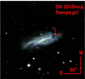
Figure 1.The𝑔𝑟 𝑖composite image of the field with the VV 525 galaxy and SN 2019muj obtained by Swope telescope at the Las Campanas Observatory.
nized composition structure (Kasen 2006). The authors argued that despite the different model, the lack of a separated secondary peak in the NIR LCs is a direct evidence for mixed ejecta structure of SNe Iax.
At the same time, the pure deflagration producing a bound rem- nant picture might contradict the bright SN Iax 2012Z (Stritzinger et al. 2015), in which the velocity distribution of intermediate mass elements (IMEs) do not indicate significant mixing in the outer ejecta.Barna et al.(2018) performed abundance tomography for a small sample of SNe Iax and found a stratified structure as a feasible solution for the outer regions of SNe Iax, however, the impact of the outermost layers are strongly affected by the choice of the density profile.
Despite the fact that the former results in this question are contradictory, constraining the chemical structure could be the key to either confirm the assumption of the pure deflagration scenario or reject it. Note that with the term (pure) deflagration we refer only on the weak deflagration scenarios hereafter, which leave behind a bound remnant (Fink et al. 2014;Kromer et al. 2015), and thus, provide a promising explanation for the SN Iax class.
A promising way to test the theory whether SN Iax share a similar origin (i.e. the pure deflagration of a CO/CONe𝑀
ChWD) is the investigation of the link between the two extremes of the Iax class, the relatively luminous and extremely faint objects. A continuous distribution of physical and chemical properties, as well as their possible correlations with the peak luminosity, favor the idea that SNe Iax may form a one (or maybe a few) parameter family. So far, these efforts are limited by the lack of well-observed, moderately luminous SNe Iax in between the extremes. The subject of our current study, SN 2019muj, now provides a good opportunity to carry out a detailed analysis of an SN Iax belongs to this luminosity gap.
The paper is structured in the following order. In Section2, we introduce SN 2019muj and give an overview of the collected data.
The light curves, spectra, and the estimated ultraviolet (UV)-optical
spectral energy distributions (SEDs) are shown in Section3. We summarize our conclusions in Section4.
2 OBSERVATIONS AND DATA REDUCTION 2.1 SN 2019muj
SN 2019muj (ASASSN-19tr) was discovered (Brimacombe et al.
2019) by the All Sky Automated Survey for SuperNovae (ASAS-SN;
Shappee et al. 2014) on 7 August 2019, UT 09:36 (MJD 58 702.4).
The location in the sky (R.A. 02:26:18.472, Dec.−09:50:09.92, 2000.0) is associated with VV 525, a blue star-forming spiral galaxy (see Fig.1) with morphological type of SAB(s)dm: (de Vaucouleurs et al. 1991) at redshift of𝑧=0.007035. Considering the low redshift, the K-correction is assumed negligible (Hamuy et al. 1993;Phillips et al. 2007). We adopted𝑑=34.1±2.9 Mpc for the distance of the galaxy fromTully et al.(2013,2016) (using the lower uncertainty value from the two studies) calculated by the Tully-Fisher method, assuming𝐻
0=70 km s−1Mpc−1. This value is slightly higher than the distance of𝑑
z=30.2 Mpc estimated from the measured redshift.
Hereafter, we use the former distance for spectral modelling and the calculation of the quasi-bolometric LC.
The SN is in the outskirts of the galaxy at a 48” projected separation (8 kpc) from its center (see Fig. 1). Because of the lack of significant Na ID line absorption at the redshift of the galaxy, we assume the host galaxy reddening at the SN position as 𝐸(𝐵−𝑉)host=0.0, while the Galactic contribution is adopted as 𝐸(𝐵−𝑉)Gal =0.023 fromSchlafly & Finkbeiner(2011). More- over, because the SN is well-separated from its host galaxy, image subtraction was not required during the data reduction.
At discovery, the apparent magnitude of SN 2019muj was 17.4 mag in theg-band. Based on the first spectrum, obtained at MJD 58702.79, the Superfit classification algorithm (Howell et al.
2005) found SN 2019muj similar to SN 2005hk around a week before maximum, thus, categorized as a SN Iax (Hiramatsu et al.
2019). These properties indicated SN 2019muj to be the brightest SN Iax with pre-maximum discovery since the discovery of SN 2014dt and intensive follow-up campaigns were started by several collaborations and observatories.
2.2 Photometry
The field of SN 2019muj was observed by the Asteroid Terrestrial- impact Last Alert System program (ATLAS; Tonry et al. 2018) before its discovery, providing a deep (∼21 mag in orange-band) non-detection limit before MJD 58 700 (see in Fig.2). The moni- toring in𝑜- and𝑐-bands continued through the whole observable time range.
The ATLAS data provide a strong constraint on the explosion epoch. ATLAS detected SN2019muj on MJD 58 702.53, just a few hours after the ASAS-SN discovery. As with all ATLAS transients, forced photometry was performed (as described inSmith et al. 2020) around the time of discovery, with the fluxes presented in TableA1 and plotted in Fig.2. There is a marginal 1.8𝜎detection on MJD 58 700.52, two days before discovery. This can either be interpreted as a detection at𝑜=20.5±0.6 mag or a 3𝜎upper limit at𝑜 <20 mag. Our analysis is not affected by either choice, as discussed further in Sec.3.1.
SN 2019muj was also observed with the Neil Gehrels Swift Ob- servatory Ultraviolet/Optical Telescope (UVOT) (hereafterSwift; Burrows et al. 2005;Roming et al. 2005) on 13 epochs between
Figure 2.The pre-maximum ATLAS photometry incyan-andorange-filters at the location of SN 2019muj. The dashed lines represent the fit of the early c-,o- andg-band LCs (latter observations are also plotted ) with power-law index n=1.3 (blue) and n=2.0 (red). Before MJD 58 700, the arrows show the 3𝜎upper limits. Note that the first detection has only 2𝜎significance.
For further details see Sec.3.1.
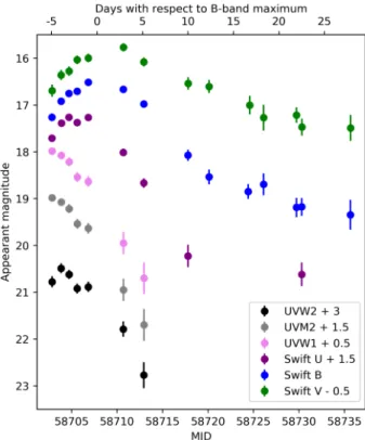
Figure 3.Swift photometry of SN 2019muj.
MJD 58 702.8 and 58 735.7. The Swiftdata were reduced using the pipeline of the Swift Optical Ultraviolet Supernova Archive (SOUSA;Brown et al. 2014), without subtraction of the host galaxy flux.Swiftlight curves (see Fig.3) provide unique UV information in UVW2, UVM2 and UVW1 filters and supplementary informa- tion to the ground-based data in𝑈 𝐵𝑉 (see TableA2). Note that flux conversion factors are spectrum dependent and the UVW2 and UVW1 filters are heavily contaminated by the optical fluxes (Brown et al. 2010,2016). This red leak may cause high uncertainties for the magnitudes of the wide bands.
MNRAS000,1–23(2020)
Ground-based photometric follow-up was obtained with the Sinistro cameras on Las Cumbres Observatory network (LCO) of 1-m telescopes at Sutherland (South Africa), CTIO (Chile), Sid- ing Spring (Australia), and McDonald (USA;Brown et al. 2013), through the Global Supernova Project (GSP). Data were reduced us- inglcogtsnpipe(Valenti et al. 2016), a PyRAF-based photometric reduction pipeline, by performing PSF-fitting photometry. Images in Landolt filters were calibrated to Vega magnitudes, and zero- points were calculated nightly from Landolt standard fields taken on the same night by the telescope, the corresponding zeropoints and color terms are also calculated in the natural system. Since the target is in the Sloan field, zeropoints for images in Sloan filters were calculated by using Sloan AB magnitudes of stars in the same field as the object. The estimated uncertainties take into account zero points noise, Poisson noise, and the read out noise.
We imaged 2019muj from MJD 58 702.5 to 58 908.0 with the Direct 4k×4k imager on the Swope 1-m telescope at Las Campanas Observatory, Chile. We performed observations in Sloan𝑢𝑔𝑟 𝑖fil- ters and JohnsonBVfilters. All bias-subtraction, flat-fielding, image stitching, registration, and photometric calibration were performed usingphotpipe(Rest et al. 2005) as described inKilpatrick et al.
(2018). No host-galaxy subtraction was performed, which would cause no significant differences, as SN 2019muj is appeared at the edge of the galaxy. We calibrated our photometry in the Swope natural system (Krisciunas et al. 2017) using photometry of stars in the same field as 2019muj from the Pan-STARRS DR1 catalog (Flewelling et al. 2016) and transformed using the Supercal method (Scolnic et al. 2015). Final photometry was obtained usingDoPhot (Schechter, Mateo & Saha 1993) on the reduced images. For better comparison, theBV magnitudes are then transformed to the Vega magnitudes (Blanton & Roweis 2007). The uncertainties are com- puted by combining the statistical uncertainties in the photometry, and the systematic uncertainties due to the calibration and transfor- mations used.
Additional optical imaging was collected by Thacher Observa- tory (Swift & Vyhnal 2018) in Ojai, CA from 9 August 2019 to 31 August 2019. The observations were taken in Johnson𝑉and Sloan 𝑔𝑟 𝑖 𝑧filters. All reductions were performed inphotpipe(Rest et al.
2005) following the same procedures as the Swope data but with photometric calibration in the PS1 system for𝑔𝑟 𝑖 𝑧and using PS1 magnitudes transformed to Johnson 𝑉 band using the equations inJester et al.(2005). In addition, the Thacher telescope camera is non-cryogenic, and so we performed dark current subtractions using 60 second dark frames obtained in the same instrumental configuration and on the same night as our science frames.
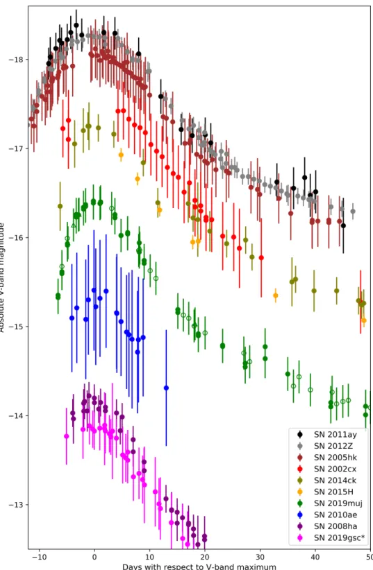
The ground-based photometric data including the 𝐵𝑉 𝑅and 𝑢𝑔𝑟 𝑖 𝑧magnitudes can be found in TablesA3andA4respectively, while the LCs are shown in Fig.4. We compare the absolute𝑉-band LC of SN 2019muj to a selection of other SNe Iax that populate the observed range of absolute magnitudes of this class in Fig.5.
2.3 Spectroscopy
Optical spectroscopy of SN 2019muj was obtained by the 9.2-m Southern African Large Telescope (SALT) with the Robert Stobie Spectrograph (RSS;Smith et al. 2006) through Rutgers University program 2019-1-MLT-004 (PI: SWJ). The observations were made with the PG0900 grating and 1.5” wide longslit with a typical spec- tral resolution𝑅 = 𝜆/Δ𝜆 ≈ 1000. Exposures were taken in four grating tilt positions to cover the optical spectrum from 3500 to 9300 Å. The data were reduced using a custom pipeline based on
Figure 4.Ground-based photometry of SN 2019muj. The filled circles, open circles, and triangles represent the observations of LCO, Swope and Thacher observatories, respectively.
standard Pyraf spectral reduction routines and the PySALT package (Crawford et al. 2010).
During the first 50 days after explosion, spectra were also obtained five times with the ESO Faint Object Spectrograph and Camera version 2 (EFOSC2,Buzzoni et al. 1984) at the 3.6-m New Technology Telescope (NTT) of European Southern Observatory as part of theePESSTO+collaboration (Smartt et al. 2015). These epochs were observed with grisms #11 (covering 3300-7500 Å and
#16 (6000-9900 Å), or #13 (3500-9300 Å) (see TableA5). The data reduction of the NTT spectra was performed using the PESSTO pipeline1(Smartt et al. 2015).
LCO optical spectra were taken with the FLOYDS spectro- graphs mounted on the 2-m Faulkes Telescope North and South at Haleakala (USA) and Siding Spring (Australia), respectively,
1 https://github.com/svalenti/pessto
Figure 5.Comparisons of absolute𝑉-band light curves of SNe Iax. References to the listed SNe Iax can be found inSzalai et al.(2015) for SN 2011ay, Yamanaka et al.(2015) andStritzinger et al.(2015) for SN 2012Z,Phillips et al.(2007) for SN 2005hk,Li et al.(2003) for SN 2002cx,Tomasella et al.(2016) for SN 2014ck,Magee et al.(2016) for SN 2015H,Stritzinger et al.(2014) for SNe 2008ha and 2010ae. Note that in the case of SN 2019gsc (Srivastav et al.
2020;Tomasella et al. 2020), the𝑉-band LC is estimated from𝑔- and𝑟-band magnitudes adopting the transformation presented inTonry et al.(2012).
MNRAS000,1–23(2020)
through the Global Supernova Project. A 2” slit was placed on the target at the parallactic angle (Filippenko et al. 1982). One- dimensional spectra were extracted, reduced, and calibrated follow- ing standard procedures using the FLOYDS pipeline2(Valenti et al. 2014).
Observations using the Kast spectrograph on the Shane-3m telescope of the Lick Observatory (Miller & Stone 1993) were made using the 2”-wide slit, the 452/3306 grism (blue side), the 300/7500 grating (red side) and the D57 dichroic. These data were reduced using a customPyRAF-based KAST pipeline3, which ac- counts for bias-subtracting, optical flat-fielding, amplifier crosstalk, background and sky subtraction, flux calibration and telluric correc- tions using a standard star observed on the same night (procedure described inSilverman, Kong & Filippenko 2020) and at a similar airmass.
Finally, two NIR spectra were taken with the FLAMINGOS-2 spectrograph (Eikenberry et al. 2008) on Gemini-South. The data acquisition and reduction are similar to that described inSand et al.(2018). The JH grism and 0.72” width longslit were employed, yielding a wavelength range of∼1.0 – 1.8𝜇m and𝑅 ∼1000. All data was taken at the parallactic angle with a standard ABBA pat- tern, and an A0V telluric standard was observed near in airmass and adjacent in time to the science exposures. The data were reduced in a standard way using theF2 PyRAFpackage provided by Gem- ini Observatory, with image detrending, sky subtraction of the AB pairs, spectral extraction, wavelength calibration and spectral com- bination. The telluric corrections and simultaneous flux calibrations were determined using theXTELLCORpackage (Vacca, Cushing &
Rayner 2020).
The optical spectra of SN 2019muj are plotted in Fig.8, while the log of the spectroscopic observations can be found in TableA5.
Our spectroscopic data were not always taken under spec- trophotometric conditions; clouds and slit losses can lead to errors in the overall flux normalization. As an example, the pupil illu- mination of SALT, moreover, changes during the observation, so even relative flux calibration from different grating angles can be difficult. Synthetic photometry of the spectra can differ from the measured photometry by a few tenths of a magnitude. For these reasons, we choose to color match all of our spectroscopic data to match the observed photometry. After this color-matching, the syn- thetic photometry of the spectra reproduces the photometric data to better than 0.05 mag across optical filters.
All the spectra are scaled and color-matched to the observed broadband photometry. Subsequently, the spectra were corrected for redshift and reddening according to the extinction function of Fitzpatrick & Massa (2007). All data will publicly released via WIseREP4.
3 DISCUSSION AND RESULTS 3.1 Photometric analysis
The ATLAS photometry provides a reliable and deep non-detection limit (𝑜 > 19.7 mag, using 3𝜎 upper limit) on MJD 58 696.58 and a marginal (2𝜎significance) detection on MJD 58 700.52 (as shown in Fig.2and Tab.A1). Assuming the so-called expanding fireball model, the observed flux increases as a quadratic function of
2 https://github.com/svalenti/FLOYDS_pipeline
3 https://github.com/msiebert1/UCSC_spectral_pipeline 4 https://wiserep.weizmann.ac.il/
Figure 6.The color evolution of SN 2019muj compared to that of SNe Iax that provide examples of more and less luminous events with respect to SN 2019muj. All magnitudes are corrected for galactic and host extinction with data taken fromStritzinger et al.(2014) for SN 2008ha andPhillips et al.
(2007) for SN 2005hk.
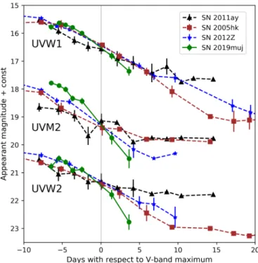
Figure 7.The observed UVW2-, UVM2- and UVW1-band light curves of SNe 2011ay (Szalai et al. 2015), 2012Z (Stritzinger et al. 2015), 2005hk (Phillips et al. 2007) and 2019muj. For better comparison, the light curves are shifted along both the horizontal and vertical axes to match at the moment of their V-band maximum.
time (𝐹 ∼𝑡2
exp) before the epoch of maximum light (Arnett 1982;
Riess et al. 1999;Nugent et al. 2011). Note that because of the lack of coverage in the first few days after explosion, the fitting of different LCs may deliver a different𝑡
exp. To determine the time of the explosion more accurately, we simultaneously fit theg-,c- ando-band LCs including the earliest observation and the best pre-
Figure 8.Spectroscopic follow-up of SN 2019muj obtained with SALT/RSS, Lick/Kast, NTT/EFOSC2 and LCO/FLOYDS spectrographs. The epochs show the days with respect to B-maximum. The observation log of spectra can be found in Tab.A5. The positions of strong telluric lines are marked with⊕.
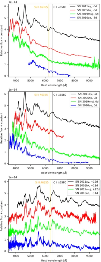
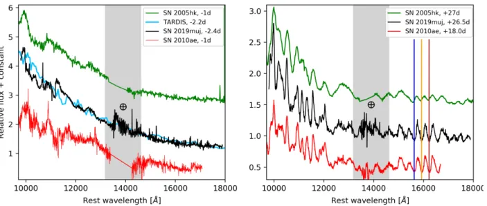
Figure 9.Comparison between spectra of Type Iax SNe 2011ay, 2005hk, 2010ae, and 2019muj obtained at similar epochs. References can be found inSzalai et al.(2015),Phillips et al.(2007) andStritzinger et al.(2014), respectively. The orange and black vertical lines show the absorption minima of the Si II𝜆6355 and C II𝜆6580 lines in the SN 2019muj spectra. With no visible absorption of the Si II𝜆6355, the orange line show its position blueshifted with 5600 km s−1(the𝑣
photof the first TARDIS model, see below).
MNRAS000,1–23(2020)
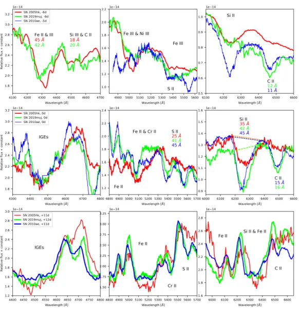
Figure 10.Zoomed insets of the spectra of SNe 2005hk, 2010ae, and 2019muj plotted in Fig.9. For better comparison, the spectra of SNe 2005hk and 2010ha are scaled to those of SN 2019muj, and also shifted to match the photospheric velocity of SN 2019muj estimated from the Doppler-shift of the C II𝜆6580 absorption. The black labels show the ions forming the prominent absorption features. In some cases, where the emission peaks provide clear delimiters for the spectral feature, the pseudo-equivalent widths of the lines are also estimated and shown with the corresponding color codes. Examples for the different pseudo-continuum are indicated with dashed lines in the plot of the Si II𝜆6355 feature in the middle row.
maximum time resolution. The fitting function is:
𝐹g=𝑎· 𝑡−𝑡
exp
𝑛
, (1)
where𝑎is a fitting parameter, while 𝑛= 2 is kept fixed at first.
The resulting date of explosion is found to be t0 =58 694.4 MJD, which seems too early regarding to the constraints provided by theo-band LC. However, another critical aspect of this analysis is the choice of power-law index. Detailed studies reported different power-law indices for samples of normal SNe Ia with mean values of n = 2.20 – 2.44 (Firth et al. 2015;Ganeshalingam, Li & Filipenko 2011). However, our pre-maximum dataset for SN 2019muj is not sufficient to handle𝑛as a free parameter, which would lead to highly unlikely results (𝑛=0.7 with constrained date of MJD 58 700.5).
As another approach, a fixed value for𝑛 <2 can be chosen.
In the case of SN 2015H,Magee et al.(2016) presented the most detailed pre-maximum LC for a SN Iax and found𝑛=1.3 as the best-fit power-law index. If we assume similarity to SN 2015H, and adopt the same vaue of𝑛for Eq.1constraining the date of explosion as MJD 58 698.1, which is a more realistic date and compatible with
the ATLAS forced photometry. Note that using𝑛=1.3 is still an arbitrary choice and no meaningful uncertainty can be estimated.
Thus, we do not claim MJD 58 698.1 as the explosion date of SN 2019muj, instead, we use it only for comparison with the results of other methods hereafter (see in Sec.3.2and3.3).
We fit the LCs with low-order polynomial functions from the first observation until two weeks after their maxima. The resulting LC parameters can be found in TableA6. According to the peak absolute magnitude in V-band, SN 2019muj is less luminous than the majority of studied SNe Iax having peak M𝑉 greater than−17 mag. Between these more luminous members of the class and the few extremely faint objects (M𝑉 >−15 mag), there is a gap of well- studied SNe Iax. According to the peak absolute magnitude (𝑀
V=
−16.42 mag), the closest relatives of SN 2019muj are SNe 2004cs and 2009J (Foley et al. 2013). However, SN 2009J has only post- maximum spectral epochs, which are insufficient to characterize the chemical properties via abundance tomography. SN 2004cs is also categorized as an SN Iax based on its only spectrum obtained at
day +42 day, andWhite et al.(2015) argue that the object does not even belong to the Iax class. Thus, SN 2019muj provides a unique opportunity to link the moderately bright SNe Iax to the brighter ones.
The estimated value of the decline rate isΔ𝑚
15 =2.4 mag in 𝐵-band and 1.0 mag in𝑟-band. These values indicate a faster dimming compared to SN 2005hk (1.56 mag in𝐵-band, 0.7 mag in 𝑟-bandPhillips et al. 2007) and all the more luminous SNe Iax with detailed photometric analysis (Foley et al. 2013). At the same time, the decline rates of SN 2019muj are comparable with those of SNe 2010ae, 2008ha (2.43 and 2.03 mag in𝐵-band; 1.01 and 1.11 mag in𝑟-band, respectively,Stritzinger et al. 2014) and 2019gsc (1.14 in𝑟-bandTomasella et al. 2020), the less energetic explosions in the class. As a conclusion, the decline rate is not well correlated to luminosity over the full range of SNe Iax.
The𝐵−𝑉intrinsic colour evolution of SN 2019muj is com- pared again to a more luminous (SN 2005hk,Phillips et al. 2007) and a fainter (SN 2008ha,Stritzinger et al. 2014) object. All SNe Iax show similar colour evolution in general (Foley et al. 2013):
the originally blue colour curve gets redder with time until 10–15 days after 𝐵-maximum, then a nearly constant color phase starts.
As can be seen in Fig.6, the𝐵−𝑉 evolution of SN 2019muj is almost identical to that of SN 2005hk over the first∼60 days. The only minor difference is the slightly bluer colour of SN 2019muj during the constant phase starting at 15 days after 𝐵-maximum.
However, the actual extent of the discrepancy is uncertain because of the highly scattered photometry at this phase. On the other hand, SN 2008ha is redder with∼0.6–0.7 mag at every epoch before the peak. It shows a similar𝐵−𝑉value of∼1.25 mag as SN 2019muj during the constant phase, though we note the lack of observations for SN 2008ha between 25 and 40 days after maximum.
SN 2019muj is only the fourth SN Iax in the literature with UV-photometry obtained by Swift. In Fig.7, the UVW2, UVM2 and UVW1 LCs are compared to those of SNe 2011ay, 2012Z and 2005hk. All three SNe are more luminous than SN 2019muj. As one can observe, the post-maximum LCs of SN 2019muj show a faster fading, which could be a sign of a steep density profile of the outer ejecta.
3.2 Spectroscopic analysis
Observed spectra of SN 2019muj are scaled and color-matched to the observed broad-band photometry. The resulting series of spectra are plotted in Fig.8, while the log of each observation is listed in Tab.A5.
In Fig.9, the spectra of three objects are compared to those of other SNe Iax that have spectra close in time to SN 2019muj and that provide examples of more and less luminous events with respect to SN 2019muj. Although the same spectral lines appear in all objects, their relative optical depths as well as the shape of the continuum vary from object to object. For better comparison, some spectral features at each epochs are displayed in the insets of Fig.
10.
At 6 days before the maximum, SN 2019muj shows only weak signs of IMEs. The spectrum over 5500 Å is nearly featureless, with C II 𝜆6580 as the only easily identifiable line. The shorter wavelengths are dominated by wide FeIIand FeIIIfeatures, which, together with the blue continuum, suggest the presence of a hot medium (𝑇 > 12 000 K) close to the assumed photosphere. The appearance of the prominent IGE lines (e.g features at∼4300 and
∼5000 Å), as well as their pseudo-equivalent widths (pEW) are strikingly similar to those of SN 2005hk (Phillips et al. 2007) at this
epoch. Note that the pEW-measurements (for a brief description see e.g.Childress et al. 2013) adopted mainly for normal SNe Ia are questionable in the case of SNe Iax, because of the the severe overlaps of the wide absorption features.
At the same time, SN 2010ae (Stritzinger et al. 2014), the extremely faint SN Iax involved in this comparison, shows strong Si II𝜆6355 line and “W” feature of SII, but restrained IGE absorption lines. These features, which typically require lower photospheric temperatures (𝑇 <11 000 K), are not identifiable in the spectrum of SN 2019muj. All these attributes make probable that SN 2019muj tends to be more similar to the more luminous SNe Iax compared to the subluminous objects of the Iax class at the pre-maximum epochs.
The only common feature in both spectra is the significant C II 𝜆6580 line, which indicates relatively high carbon abundance in the outermost region of SN 2019muj. However, the limited wavelength range of the spectrum of SN 2010ae (and the lack of spectra of other extremely faint SNe Iax at this epoch) makes this comparison incomplete.
The match changes around the maximum when the structures and the estimated pEWs of the IME features of SN 2019muj re- semble more closely those of SN 2010ae, than those of SN 2015hk.
The strength of the C II𝜆6580 feature still provide a good match with that of SN 2010ae, while this feature is barely identifiable in the spectrum of SN 2005hk. At the same time, the IGE dom- inated absorption feattures below 6000 Å show a diverse nature.
The pseudo-emission peaks between 4300 and 4700 Å are in better agreement with the same features of SN 2005hk, while the more narrow Fe II absorption lines between 4700 and 5150 Å are more similar to those of SN 2010ha. At∼12 days after the maximum, the whole range spectral range of SN 2019muj is nearly a perfect match to that of SN 2010ae, while the SN 2005hk spectrum shows several more dominant pseudo-emission peaks (e.g. at 4700 and 5700 Å.)
The different nature of SN 2019muj before and after maximum light might be the result of the steeper density structure. The thin outer region allows insight to the deeper, thus, hotter layers, which changes as the photosphere starts forming in the more dense regions.
Such density structure may resemble more with that of the more luminous objects in the outer region with a cut-off at the highest velocities (see the N5def and N20def deflagration models and the abundance tomographies of SNe Iax,Fink et al. 2014;Barna et al.
2018), and the profile quickly increase toward the innermost regions (see the N1def and the hybrid N5def deflagration models,Fink et al.
2014;Kromer et al. 2015). It can not be stated whether this behavior is regular among the moderately luminous SNe Iax, or not, without studying more objects with approximately the same luminosity.
The best candidates for this purpose are SNe 2014ck (Tomasella et al. 2016) and 2015H (Magee et al. 2016) so far, both SNe had a relatively moderate luminosity (still a magnitude brighter than SN 2019muj) and detailed observational data. However, constraining the density profile (see below) of multiple objects is beyond the scope of this study.
In order to test the physical structure of the ejecta, we fit the spectral time series with synthetic spectra calculated via the 1D Monte Carlo radiative transfer codeTARDIS(Kerzendorf & Sim 2014;Kerzendorf et al. 2019;Vogl et al. 2019) in multiple ways.
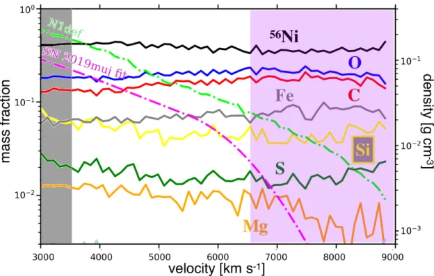
First, we use the abundance template proposed by Barna et al.
(2018) for the sample of more luminous SNe Iax. The template (see Fig.11) is paramterized by a velocity shift of the abundance struc- ture, measured by the velocity where the56Ni abundance becomes dominant. In the case of 2019muj, we use this velocity shift of the abundance template as a free parameter for fitting the spectra. The assumed density function is the same as those used byBarna et al.
MNRAS000,1–23(2020)
Figure 11.The adopted abundance template fromBarna et al.(2018) shifted with 6500 km s−1(i.e. the transition velocity between the56Ni dominated inner and the O dominated outer regions). The green, cyan and magenta dashed lines represent the density profiles of the N1def (Fink et al. 2014), the N5def_hybrid (Kromer et al. 2015), and the feasible fitTARDISmodel (this paper) scaled to texp= 100 s, respectively. Note that the lack of earlier spectra and the steep cut-off in the adopted density profile above∼6500 km s−1makes the constraints on abundance structure uncertain in this outer region (highlighted with purple area).
Moreover, the latest TARDIS model has photospheric velocity of 3600 km s−1, thus, we cannot test the chemical abundances below this limit (highlighted with grey area).
Figure 12.The chemical abundances of the N1def pure deflagration model (Fink et al. 2014) as comparison to Fig.11. The density profiles of N1def and our TARDIS model are also shown with dashed lines. Similarly to Fig.11, the uncertain (above∼6500 km s−1) and unseen (below 3600 km s−1) regions are highlighted with purple and grey colors, respectively.
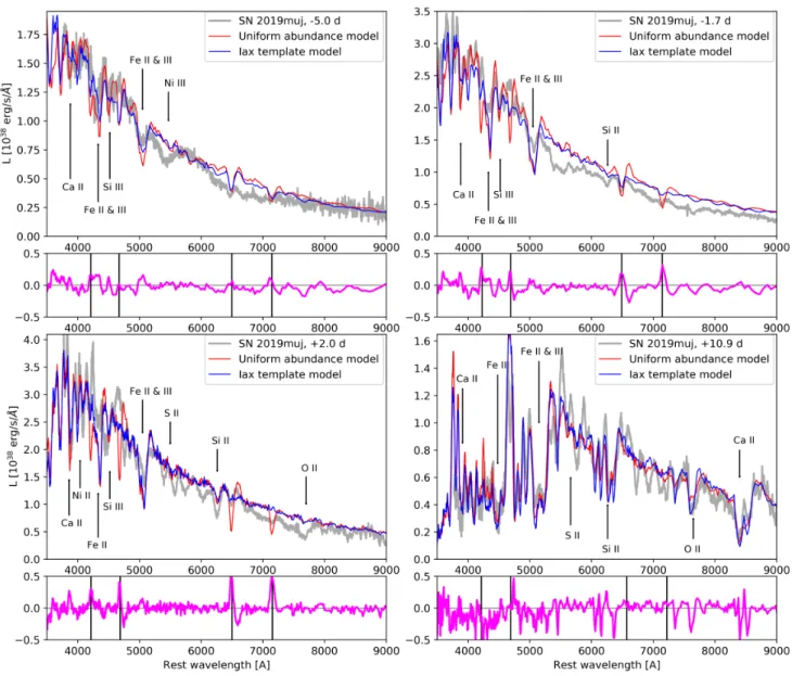
Figure 13.Four of the observed spectra of SN 2019muj obtained around maximum (grey), corrected for reddening and redshift, theTARDISsynthetic spectra assuming the abundance template fromBarna et al.(2018) (blue) and the impact of assuming uniform abundances based on the N1def model fromFink et al.
(2014) (red). The purple residuals show the difference between the two synthetic spectra in each panel. Vertical lines indicate the absorption minima of the C II lines𝜆4268,𝜆4746,𝜆6580 and𝜆7234 in the residual plots. Key spectral lines formed by other ions in the template model are indicated by black arrows.
(2018, note that the related Eq. 1 in the cited paper is incorrect) for reproducing the density structure of various deflagration models ofFink et al.(2014). The density function contains an exponential inner part, which continues with a shallow cut-off past the velocity 𝑣cut:
𝜌(𝑣 , 𝑡
exp)=
𝜌0·𝑡
exp 𝑡0
−3
·exp
−𝑣𝑣
0
for𝑣≤𝑣
cut
𝜌0·𝑡
exp 𝑡0
−3
·exp
−𝑣𝑣
0
·8
−8(𝑣−𝑣cut)2 𝑣2
cut for𝑣 > 𝑣
cut
(2) where𝜌
0is the reference density at the reference time of𝑡
0 =100 s,𝑣is the velocity coordinate and 𝑣
0 is reference velocity, which defines the slope of the density profile. In our fitting strategy, we use 𝜌0,𝑣
0and𝑣
cutas free parameters, while the date of the explosion
is adopted from the LC analysis. Luminosities and photospheric velocities are constrained individually for each spectrum.
Note that our approach of spectral fitting is only a simpli- fied version of the technique called abundance tomography (Stehle et al. 2005), because the chemical abundances are controlled via the template. Moreover, our fitting strategy does not result in a
‘best-fit’ model, because the whole parameter-space cannot be fully explored manually. Instead, we aim to find a feasible solution for the main characteristics of SN 2019muj assuming physical and chemi- cal structure which reproduced the main spectral features of several epoch in the case of more luminous SNe Iax.
We find a feasible solution assuming explosion date of MJD 58 697.5±0.5, which is in good agreement with the previously estimated value from the early LC fitting (MJD 58 698.1). The core density is assumed to be 𝜌
0 = 0.55 g cm−3, while the slope of the function in the inner region is𝑣
0 = 1800 km s−1. The density MNRAS000,1–23(2020)
Figure 14.The two infrared spectra obtained with Gemini-South/FLAMINGOS-2 spectrograph, compared to to Type Iax SNe 2005hk (Kromer et al. 2013) and 2010ae (Stritzinger et al. 2014) obtained at similar epochs. The TARDIS synthetic spectrum fitted to the optical spectrum and extended to the longer wavelengths is also plotted in the first panel. The epochs show the days with respect to𝐵-band maximum. The blue, orange and brown vertical lines show the absorption minima of the Co II𝜆15795,𝜆16064 and𝜆16361 lines for the second epoch. The wavelength range heavily affected by major telluric absorption lines are marked with grey stripe.
profile starts to deviate from the pure exponential function above 𝑣cut= 5500 km s−1. In accord with the expectations based on the loose correlation between the ejecta structure and the luminosity, these parameters are lower for SN 2019muj compared to those of previously analyzed SNe Iax (Barna et al. 2018). The constructed density profile also falls short of reaching the density function of the N1def model (Fink et al. 2014), but stays above the density function of the N5def_hybrid model (Kromer et al. 2015), directly developed for a possible explanation of the extremely faint SNe Iax (Fig.11). Note that the photospheric velocity of the latest TARDIS model of this analysis limits the part of the ejecta we can study.
Thus, we cannot gain any knowledge neither about the density or the chemical abundances below 3600 km s−1.
As it was indicated in Sec.1, the impact of the outer regions on the synthetic spectrum strongly depend on the choice of density at high velocities. The adopted density profile has a steep cut-off above∼6500 km s−1(see in Fig.11), which makes the abundance structure highly uncertain in this region. Thus, one should test, whether the abundances of specific chemical elements are indeed sensitive to the outermost velocity region. After constraining the set of fitting parameters for the abundance template, we calculate synthetic spectra with constant abundances using the same physical properties. The mass fractions of these models are adopted from the N1def model ofFink et al.(2014) (see in Fig.12), averaging and normalizing the abundances of the chemical elements listed in Fig.11. The comparison between the two sets of synthetic spectra is plotted in Fig.13.
The template models show a relatively good agreement with the observed spectra, especially a week after maximum light, where the synthetic spectra reproduce almost all the absorption features.
At the earliest epochs, an excess of carbon is found despite the mass fraction decrease inward of the photosphere. This suggests that stronger limitation of carbon abundance is required to produce the spectral lines correctly. Around maximum light, the absorption features of IMEs do not or just slightly appear, which may require a more complex treatment of the temperature and density profile.
At the same time, the spectra calculated from the constant abundance model match similarly well to the observed data, apart from the spectral features of C II (see Fig.13). Due to the steep cut- off in the adopted density profile, testing the ejecta structure far over the photosphere of the first epoch (𝑣
phot=6 000 km s−1) is highly uncertain as it is indicated in Figs.11and12. In the regions probed in our work we cannot tell the difference between the stratified and constant abundance model as our spectra do not go early enough, except in the case of carbon. As it is shown in Fig.13, carbon forms too strong absorptions in the case of the constant abundance model around the maximum light. This exceed in the uniform abundance models would result from the relatively high 𝑋(𝐶) ≈ 0.13 mass fraction below 6000 km s−1 in the constant profile. This confirms the assumption ofBarna et al.(2018) that a significant amount of unburned material in the ejecta of SNe Iax is likely found only in the outermost layers.
As a result, our analysis seems to favour the implied a stratified structure over the constant abundance model, as stratified abundance profile is required to reproduce the main spectral features of car- bon. In the case of other chemical elements, the differences between the two models can be probed only with earlier spectral observa- tions. Apart from carbon, the uniform abundance profiles of the N1def model describe well the chemical structure of SN 2019muj in general. Considering the possible explosion scenarios (see Sec.
1), which can explain some of the observables of SNe Iax, the constrained abundance profiles of SN 2019muj may not contradict strongly with the predictions of the pure deflagration scenario, but definitely require some further tuning in the hydrodynamic models at least in the case of unburned material.
The self-consistentTARDISmodels also provide us an estima- tion of the photospheric velocity based on the simultaneous fits of several spectral lines and the flux continuum. The evolution of vphot is monotonically decreasing, with a steeper descent before the mo- ment of the maximum light. The derived behaviour of vphot(see Fig.
15) shows good agreement with the average velocity estimated from the blueshift of the SiII𝜆6355 absorption minima. Moreover, the
Figure 15.The evolution of photospheric velocity of SN 2019muj (𝑀 V=
−16.42 mag) and five relatively bright SNe Iax (Barna et al. 2018) with peak absolute brightness covering a range from−17.3 (SN 2015H) to−18.4 mag (SN 2011ay). The velocities (illustrated with filled circles) were con- strained via abundance tomography analysis performed withTARDIS. The photospheric velocities of the extremely faint SN 2019gsc (𝑀
V∼ −13.8 mag) constrained via spectral fitting withTARDISare also plotted (Srivastav et al. 2020). The crosses (between 5 and 221 days) and the star (at 34.4 days) show the photospheric velocity estimated from the shift of the absorption minima of Si II𝜆6355 and the NIR Co II lines, respectively.
vphotof the CoIIfeature in the NIR regime at +26.5 days also sup- ports this velocity evolution. The velocity profile of SN 2019muj fits into the trend of other SNe Iax, which showed a relation be- tween the peak luminosity and the value of vphot at V-maximum (McClelland et al. 2010;Foley et al. 2013). This result suggests that this correlation is tight not only for the most luminous SNe Iax, but probably for the whole class. However, to achieve more general conclusions regarding to the luminosity-velocity relation, more SNe Iax (including the reported outliers, e.g. SNe 2009ku and 2014ck, Narayan et al. 2011;Tomasella et al. 2016) have to be studied with the same technique.
The velocity estimation could be further improved by analyz- ing the near-infrared (NIR) spectral features. The two spectra of SN 2019muj obtained in the NIR regime are shown in Fig.14. There are only a few SNe Iax with near-infrared (NIR) spectra: such obser- vations have been presented in the case of SNe 2012Z (Stritzinger et al. 2015), 2005hk (Kromer et al. 2013), 2008ge (Stritzinger et al.
2014), 2014ck (Tomasella et al. 2016), 2015H (Magee et al. 2016) and 2010ae (Stritzinger et al. 2014). Although TARDIS modeling is unreliable for fitting spectra at infrared wavelengths due to the black body approximation, the synthetic spectra could be used for identifying spectral features. Thus, we shift the flux of the TARDIS synthetic spectrum created for the -1.7 day epoch to match with the -2.4 day NIR spectrum. The shape of the continuum is of the synthetic and observed spectra are surprisingly similar, despite that real flux of the the synthetic spectrum is scaled with approximately an order of magnitude. However, the synthetic spectrum shows very weak spectral lines, which mostly overlap each other, making the precise line identification unfeasible. Note that the epoch of the lat- est optical spectrum fit with our TARDIS is 10.9 days after B-band maximum, thus, the comparison for the second NIR spectrum is not possible.
In Fig.14, we also compare the two NIR spectra of SN 2019muj
Figure 16.The SED of SN 2019muj calculated from UV/optical photometry at three different epochs, compared to the spectra obtained at the closest epochs (grey and black). The epochs indicate the time with respect to𝐵- band maximum (MJD 58 707.8). The flux values estimated from the Swift UVW2 and UVW1 bands are represented by two green points on each panel.
to those of SNe 2005hk and 2010ae obtained at similar epochs. Al- though, even the two comparative spectra are very similar at few days before the maximum light (it was also shown byStritzinger et al. 2014), there are some differences between 10 000 and 12 000 Å dominated by Mg II and Fe II lines (Tomasella et al. 2016), where the absorption features are stronger, especially those at∼11 300 Å, which barely noticeable in the spectrum of SN 2019muj. These properties make SN 2019muj resembling to the more luminous SN 2005hk at the earlier epoch. Similarly to the optical spectral evolu- MNRAS000,1–23(2020)
Figure 17.The bolometric LC of SN 2019muj and the best-fit Arnett-model described with Eq.3. The light curve peaks at MJD 58707.2. For comparison, the UVOIR LC of the N1defFink et al.(green,2014) and N5def_hybdrid Kromer et al.(cyan,2015) deflagration models are also plotted.
tion (Fig.9), SN 2019muj at NIR wavelengths also turns to be more similar to the fainter SN 2010ae, as their spectra obtained at few weeks later (+26.5 and +18 days, respectively) are almost identical.
At these epochs, the most prominent NIR features are the set of CoIIlines, which appear with significantly lower relative strength in the spectrum of SN 2005hk. The CoIIfeatures do not overlap and allow us to measure the photospheric velocity with at post- maximum epochs (Stritzinger et al. 2014;Tomasella et al. 2016).
Among the reported lines, CoII𝜆15795,𝜆16064 and𝜆16361 can be easily identified in the later NIR spectrum of SN 2019muj. Based on the blueshifts of the absorption minima, the photospheric veloc- ity is𝑣
phot =2500 km s−1at+26.5 days after𝐵-band maximum light. We compare this value with other methods to investigate the evolution of the photosphere below.
3.3 Bolometric light curve and SED
We calculated F𝜆flux densities from theSwift,𝑈 𝐵𝑉and𝑔𝑟 𝑖dered- dened magnitudes based on Bessel, Castelli & Plez (1998) and Fukugita et al.(1996), respectively, and created SEDs for several epochs. Note thatSwiftwide band magnitudes are not used for this calculation, because of the potentially high uncertainties (see Sec.
2.2). For a given date, if SN 2019muj was not observed in some of the filters, we use the corresponding value from the fitting of a low-order polynomial function to the observed magnitudes. The SEDs are directly compared to the spectra (corrected for reddening) in Fig.16. Integrating the SED functions to the total flux and scaling it according to the assumed distance, a quasi-bolometric LC is es- timated (Fig.17). The derived luminosities are fit with the analytic LC model introduced byChatzopoulos, Wheeler & Vinkó(2012), which is based on the radioactive decay diffusion model ofArnett (1982) andValenti et al.(2008). The function has the following form:
𝐿(𝑡)=𝑀
Ni·exp
−𝑥2
· h
1−exp
−𝐴/𝑡2 exp
i
·h (𝜖
Ni−𝜖
Co)
∫ 𝑥
0
2𝑧·exp
𝑧2−2𝑧 𝑦
𝑑 𝑧
+𝜖
Co
∫ 𝑥
0
2𝑧·exp
𝑧2−2𝑧 𝑦+2𝑧 𝑠
𝑑 𝑧 i
(3)
where𝑡
exp is the time since the explosion, MNiis the radioactive nickel mass produced in the explosion, while𝜖
Coand𝜖
Niare the energy generation rates by the decay of the radioactive isotopes of cobalt and nickel. Gamma-ray leakage from the ejecta is considered in the last term of the equation, where 𝐴 = (3𝜅𝛾𝑀
ej) / (4𝜋𝑣2) includes the gamma-ray opacity𝜅𝛾, the expansion velocity𝑣and the mass of the ejecta𝑀
ej. The additional parameters are𝑥=𝑡/𝑡
d, 𝑦=𝑡
d/ (2𝑡
Ni),𝑧=1/2𝑡
d, and𝑠=𝑡
d· (𝑡
Co−𝑡
Ni)/(2𝑡
Co𝑡
Ni), where tdis the effective diffusion time.
The fit of the bolometric LC is plotted in Fig.17, while the best-fit parameters are listed in TableA7. The date of explosion is found as MJD 58 698.2±0.5. This is in good agreement with the date estimated from the spectral fitting (MJD 58 697.5±0.5) and almost perfectly matches with the estimated value from the early LCs (MJD 58 698.1). Accepting MJD 58 698.2 as opposed to the one provided by the fireball model allows us to adjust the power- law fit of the early LCs, yielding𝑛≈1.26. The rise times of SNe Iax are significantly shorter than those of normal SNe Ia, and this trend is confirmed in SN 2019muj, with𝑡
rise = 9.6±0.6 days in the𝐵-band (see Tab.A6). SN 2019muj also fits well to the trend of SNe Iax showing a loose correlation between their rise times and peak absolute magnitudes (see e.g.Tomasella et al. 2016;Magee et al. 2016, for V- and r- band comparisons).
Based on the bolometric LC fit, the amount of56Ni produced during the explosion (MNi=0.031±0.005 M) is low, even within the Iax class. It is approximately half of the estimated nickel mass of SN 2015H (0.06 M,Magee et al. 2016),∼30% of that of SN 2014ck (0.1 M,Tomasella et al. 2016) and only∼14% of that of the brightest type Iax SN 2011ay (0.225 M,Szalai et al. 2015).
At the same time, this nickel mass is an order of magnitude higher than those of the extremely faint SNe 2008ha and 2019gsc (0.003 𝑀,Foley et al. 2013;Srivastav et al. 2020), which confirms the placement of SN 2019muj in the gap of the luminosity distribution of SNe Iax. Nevertheless, the initial56Ni mass of SN 2019muj matches reltively well with the value of MNi=0.0345 Mof the N1def pure deflagration model calculated byFink et al.(2014) via hydrodynamical simulations. The similarity to N1def occurs not just on the peak brightness, but also on the post-maximum evolution of the LC (Fig.17). This match further supports the idea that despite the possible discrepancies in the chemical abundances, SN 2019muj is the product of the pure deflagration scenario.
Assuming a correlation between𝑀
ejand𝑀
Nias in the model grid ofFink et al.(2014), we may set the 𝑀
ej = 0.0843 M of the N1def model as an upper limit for SN 2019muj. Note however that the synthetic LCs of these pure deflagration models decline too rapidly compared to the SNe Iax LCs. The increased transparency of the ejecta is probably the simple consequence of the insufficient ejecta masses in the hydrodynamic simulations. Another method was proposed byFoley et al.(2009) taking advantage that both the rise time and the expansion velocity are proportional to the ejecta mass (Arnett 1982), which leads to:
𝑀ej∝𝑣
exp×𝑡2
rise. (4)
Assuming that the mean opacity of the ejecta is uniform among thermonuclear SNe, this simplification allows to estimate the ejecta mass by comparing the bolometric rise time (𝑡
rise=9.0 days, see in Fig.17) and expansion velocity (here we adopt𝑣
exp=5000 km s−1) to those of normal SNe Ia. Following the formula presented by Ganeshalingam et al.(2012), we estimate𝑀
ej=0.17 M, while the kinetic energy of the ejecta is𝐸
kin=4.4×1049erg. The discrepancy between ejecta masses calculated by this method and that of N1def deflagration model assumed as upper limit for SN 2019muj is similar