On the Persistence of the Electromagnetic Field

On the Persistence of the Electromagnetic Field

Márton Gömöri

László E. Szabó

∗Institute of Philosophy, Research Center for the Humanities, Hungarian Academy of Sciences, Budapest

∗∗Department of Logic, Institute of Philosophy, Eötvös University, Budapest

Abstract

According to the standard realistic interpretation of classical electro- dynamics, the electromagnetic field is conceived as a real physical entity existing in space and time. The problem we address in this paper is how to understand this spatiotemporal existence, that is, how to describe the persistence of a field-like physical entity like electromagnetic field.

First, we provide a formal description of the notion of persistence: we derive an “equation of persistence” constituting a necessary condition that the spatiotemporal distributions of the fundamental attributes of a persist- ing physical entity must satisfy. We then prove a theorem according to which the vast majority of the solutions of Maxwell’s equations, describ- ing possible spatiotemporal distributions of the fundamental attributes of the electromagnetic field, violate the equation of persistence. Finally, we discuss the consequences of this result for the ontology of the electromag- netic field.

1 Introduction

There is a long debate in contemporary metaphysics whether and in what sense instantaneous velocity can be regarded as an intrinsic property of an object at a given moment of time (Butterfield 2006; Hawley 2001, pp. 76–80; Sider 2001, pp. 34–35; Arntzenius 2000; Tooley 1988). What is important from this debate to our present concern is—in which there seems to be a consensus—that

[T]he notion of velocity presupposes the persistence of the object concerned. For average velocity is a quotient, whose numerator must be the distance traversed by the given persisting object [. . .]

So presumably, average velocity’s limit, instantaneous velocity, also presupposes persistence. (Butterfield 2005, p. 257).

We will argue in this paper that the opposite is also true:persistence presupposes velocity. More precisely, as we will see, in case of a spatially extended physical object, persistence presupposes, at least, the existence of a field of local and instantaneous velocity; regardless if this local instantaneous velocity is consid- ered as an intrinsic property of the object concerned, or not. Velocity occurs as

1

a “kinematic” feature of the way in which the object persists. This is in accor- dance with our natural intuition: if a material object like a small particle exists, it exists in space and time; if it persists, it must occur somewhere in space at different moments of time. So it must have some (not necessarily non-zero) average velocity characterizing its spatiotemporal existence.

In section 2 we give a formal description of persistence in terms of the spa- tiotemporal distributions of quantities that track the identity of the persisting object through time. We derive an “equation of persistence” constituting a nec- essary condition the distributions of tracking quantities must satisfy in every space-time point where the extended object persists. It turns out however that this condition is not necessarily satisfied by some field-like physical entities.

In section 3 we discuss the case of electromagnetic field. We show that the equation of persistence is satisfied in some particular states of the electromag- netic field. This is however the exception: we will prove a theorem according to which the vast majority of the solutions of Maxwell’s equations violate the equation of persistence. In section 4 we discuss the possible consequences con- cerning the ontology of electromagnetic field.

2 Formal description of persistence

Physics literature has practically no explicit discussion of the problem of per- sistence. There must be however an implicit intuition of persistence behind such everyday notions of physics as the velocity of a moving object, the world line or world tube of a material body, the lifetime of a particle, the track of a particle in a cloud chamber, the speed of a neutrino, the deformation of a rod, the cooling of a hot iron ball, etc. If these notions make sense at all – without which there would be no meaningful physical theory – there must be a sense of persistence; some criteria,some facts of the physical world, that entitle the physicist to say that the substance occupying regionAat momenttand the one occupying region A^∗ att^∗ constitute the same physical object. Claims of this sort, in which we assert that an object existing at one time is the same object as the one existing at some other time, are called claims of diachronic sameness.

Metaphysicians offer two major interpretations of persistence: endurantism and perdurantism. According to endurantism a concrete particular persists through time by existing wholly and completely at each moment of time of its existence. In other words, persistence through time is construed as thenu- merical identityof a thing existing at one time with a thing existing at another time. As opposed to endurantism, according to perdurantism assertions of di- achronic sameness are not assertions of literal identity at all; a concrete partic- ular is constituted by a sequence ofnumerically different temporal parts(phases, stages, or temporal slices). Endurantism is usually combined with presentism or three dimensionalism, while perdurantism with eternalism or four dimen- sionalism.

Although it is not at all obvious what the final ontology of the world is ac- cording to our best physical theories (e.g. Kuhlmann 2015), it is not far from the truth to say that the world view of contemporary physics is closer to per- durantism + four dimensionalism.

Perdurantism + four dimensionalism (also called “worm-view”) has to explain how temporal “parts”, as independent entities, constitute a four-

Figure 1: Which head belongs to which tail? Entity A is obviously not similar to entity D in all respects; as A is a head and D is a tail, for example. But the fact that A belongs to the same caterpillar as D entails that some intrinsic properties of A and D are common; for example, the cells in A and D have the same genome. What is true about the spatial parts is true about the temporal parts. The fact that caterpillar AD is the same being as butterfly F entails that they have the same genome.

dimensional “whole”. In other words: what makes the “temporal parts” parts of one and the same four-dimensional object? The dominant views are based on three components: spatiotemporal continuity, qualitative similarity, and causal relations. The crucial question is how qualitative similarity should be understood. Qualitative identity, the maximal level of qualitative similarity, can be too strong a requirement for diachronic sameness; arbitrary kind and level of qualitative similarity can be too weak. Further restrictions to qualita- tive similarity might be needed (e.g. Swartz 1991, pp. 337–357).

It is not our intention, however, to give a general criterionsufficientfor di- achronic sameness. For our present purposes we only need to assume that, in every particular case, there issomelevel of qualitative similarity that isneces- saryfor diachronic sameness. To make explicit what we mean by the “necessary level of qualitative similarity”, we stipulate the following.

Tracking principle If two things in region A at moment t and in region A^∗ at t^∗are the same physical object, then there is a certain package of tracking properties intrinsic to both things, in region A at time t and in region A^∗at time t^∗.

That is to say, diachronic sameness is tracked by sameness in some key prop- erties. This claim quadrates with the wider metaphysical view that qualitative similarity should be understood as “partial identity” (e.g. Heil 2003, p. 156).

Literally speaking, the tracking principle, as a necessary condition for di-

achronic sameness, is also compatible with endurantism. It simply follows from the Leibniz principle: if two things in two different spatiotemporal re- gions are numerically identical, then, by the indiscernibility of identicals, they must have allproperties in common; a fortiori,they must sharesomeof their properties. (It is not our concern here to discuss the tension between diachronic identity, the Leibniz principle, and change in time.)

First of all, however, the tracking principle can be learned from the prac- tice of physics. For when the physicist asserts that the particle emitted here is the same particle as the one detected over there, what she asserts is the exis- tence of some key properties—the particle’s mass, charge, spin, lepton number, etc.—instantiated both at the events of emission and detection. (Consider the analogy depicted in Fig. 1.) When the physicist talks about velocity, world line, lifetime, deformation, etc.—notions that presuppose the persistence of a physical object—, there always exists a package of key intrinsic properties char- acterizing the object in question in terms of which the physicist can express its diachronic sameness. In fact, from a physics point of view, each particular ap- plication of the tracking principle can be conceived as a part of the constitutive a priori¹that provides thevery meaningof a physical term like velocity, world line, lifetime, deformation, etc. Again, it must be emphasized that the tracking principle, even when conceived as a constitutive principle for physics, is only supposed to specify anecessarycondition for identity through time, butnota sufficient one. Two electrons have the same intrinsic properties, but in many cases the physicist is able to discern them based on other considerations like spatiotemporal continuity.

From metaphysical point of view, the difference between necessity and suf- ficiency is even more fundamental. Imagine a particle moving along a path.

Assume that the particle is annihilated at a moment of time; and, immediately, anotherparticle is created with exactly the same intrinsic properties, continuing along the same path. (‘Another’ means ‘numerically distinct’ for the enduran- tist, and ‘belonging to a different worm’ for the perdurantist.) As this example shows, even if spatiotemporal continuity is provided, and even if the pack- age of tracking properties covers all intrinsic properties (qualitative identity), the tracking condition does not constitute a sufficient metaphysical criterion of diachronic sameness.

Note also that the principle says nothing about the content of the package of tracking properties in question. In particular, it is not necessarily identical with the complete package of properties determining the synchronic identity of the object; neither in the sense of a four-dimensional worm, nor in the sense of its temporal parts in region Aat timetor in regionA^∗at timet^∗. Further, the existence of such a package does not imply that the object cannot change in time: it can change in all the various properties not contained in the tracking package. (Consider again the analogy depicted in Fig. 1.)

In what follows we shall translate the condition provided by the tracking principle to mathematical terms. Without loss of generality we may assume that each of the tracking properties in question can be characterized as such that a certain (real valued) quantity fitakes a certain value; more precisely, the spatiotemporal distribution of this quantity, fi(r,t), takes a certain local value at a spatiotemporal locus. Accordingly, we are going to express a necessary

1In the sense of Reichenbach 1965.

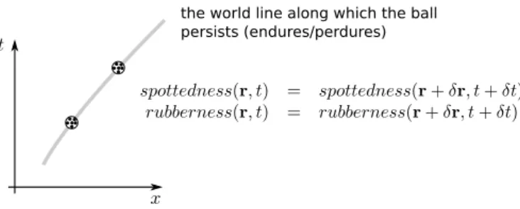
the world line along which the ball persists (endures/perdures)

Figure 2:A small, “point-like” ball can be tracked by its spottednes, rubberness, etc.

condition for diachronic sameness in terms of these distributions of tracking quantities. We proceed in three heuristic steps.

I.

First we consider the persistence of a point-like physical object.

Let f1,f2, ...,fnbe the package of tracking quantities. In line with the track- ing principle we assume that

fi(r,t) = fi(r^∗,t^∗) (1)

(i=1, 2, . . . ,n)

for any two points(r,t)and(r^∗,t^∗)along the world-line of the persisting object (Fig. 2). Introducing theaverage velocityasv= ^r_t^∗∗^−r−t, we can write:

fi(r,t) = fi(r+vδt,t+δt) (2) (i=1, 2, . . . ,n)

withδt=t^∗−t.

Assume that all functionsf₁,f2, ...,fnare smooth (if not, they can be approx- imated as closely as required for physics by smooth functions). Taking (2) for a small, infinitesimal interval of time, and expressing it in a differential form—by which, moreover, we comply with the required spatiotemporal continuity—we have

−∂_tfi(r,t) = ∇fi(r,t)·v(t) (3) (i=1, 2, . . . ,n)

wherev(t)is the instantaneous velocity. In components:

−∂_tfi(r,t) = Vx∂_xfi(r,t) +Vy∂_yfi(r,t) +Vz∂_zfi(r,t) (4) (i=1, 2, . . . ,n)

Of course, the concrete world-line along which the object persists may be var- ied. Thus, equations (3) with some instantaneous velocity constitute anecessary condition the tracking quantities must satisfy in every space-time point where the object persists. Let us call them theequations of point-like persistence.

the world tube in which the ball persists (endures/perdures)

Figure 3: A spotted ball, as an extended object, can be characterized by the distribu- tions of whiteness and blackness

II.

Now we make a straightforward extension of the above results to the case of a spatially extended object. Assume that the fine-grained structure of an extended object also can be described in terms of the distributions of some, probably more fundamental, quantities (Fig. 3). And, therefore, the diachronic sameness of the persisting object can be tracked in terms of a suitable pack- age of these distributions, f1,f2, ...,fn. It is a straightforward generalization of the idea expressed in equation (3) to say that if an extended object persists then there must exist a velocity vectorv(t)for every moment of time, such that equation (3) is satisfied in all space-time points (r,t)belonging to the space- time tube swept by the extended object.

However, this describes only a particular situation when the extended ob- ject persists like a rigid body in translational motion. The instantaneous ve- locityv(t)is the same everywhere in the spatial region occupied by the object.

Consequently, the spatial distributions f_i(r,t = const)are simply translating with a universal velocity, without deformation. Of course, generally this is not necessarily the case. For example, the ball in Fig. 4 preserves its identity even though it rotates and inflates.

III.

Concerning the general case, imagine an extended object with a more complex behavior. LetΣtandΣt+δtdenote the spatial regions occupied by the object at timetandt+δt. The object can change in various senses. Even ifΣt =_Σt+δt, the spatial distributions of its local properties may change, in the sense that for several distributions f_i(r,t) 6≡ f_i(r,t+δt). Moreover,ΣtandΣt+δtmay differ not only in their location but also in size and shape. All these changes manifest themselves in the spatiotemporal distributions of local properties, that is, in the distributions fi(r,t). For example, all changes, the translation, the rotation, and the inflation of the ball in Fig. 4 are expressible in terms of the distributions

( )

( )

the world "tube" in which the ball persists (endures/perdures)

Figure 4:The ball preserves its identity even though it may rotate or inflate

likewhiteness(r,t)andblackness(r,t).

Now, how can we describe the persistence of such an object? What con- ditions the distributions fi(r,t)must satisfy in order to count the two things inΣtand Σt+δt as identical, or as two temporal parts of the same object? In line with the tracking principle, the conditions we are looking for have to ex- press, in terms of a relation between the values of f_i(_r,t)_inΣtand the values of f_i(r,t+δt)in Σt+δt, thatΣt and Σt+δt share some key properties. On the basis of our previous considerations in points Ior IIand the examples like the inflating-rotating ball, we claim that the general form of such conditions is the following. There must exist a package of relevant, tracking distributions

f₁,f2, ...,fnand a mappingϕ_t,t+δt:Σt→_Σt+δt, such that

fi(r,t) = fi(ϕ_t,t+δt(r),t+δt) (5) (i=1, 2, . . . ,n)

(5) expresses the metaphysical intuition that the extended object can be con- ceived as the mereological sum of its “local parts”, each of which itself being a persisting entity, whose identity over time is described by function ϕ_t,t+δt. Notice that the only non-trivial requirement imposed on ϕt,t+δtby (5) is that it must be common for all tracking distributions fi(r,t). Intuitively this means that if a local part of the object atrinstantiates some local tracking properties then its counterpart at pointϕ_t,t+δt(r)instantiates the same local tracking prop- erties—in harmony with the tracking principle’s requirement. Note however that this fact by no means implies that the extended object necessarily consists of atomic entities—pointlike or non-pointlike—persisting in the sense of points IorII. Just the contrary, the general notion of persistence defined by (5) satis- fies a kind of downward mereological principle: if the whole extended object persists in the sense of (5) then all (arbitrarily small) local parts of the object persist in the same sense.

Assuming that ϕ_t,t+δt(r)is smooth and ϕt,t = id_Σt—by which we, again, comply with spatiotemporal continuity—, one can express (5) in the following

differential form:

−∂_tfi(r,t) = ∇fi(r,t)·v(r,t) (6) (i=1, 2, . . . ,n)

wherev(r,t) =∂t^∗ϕt,t^∗

t^∗=t

(r). v(r,t)can be interpreted as the instantaneous velocity field characterizing the motion of the local part of the extended entity at the spatiotemporal locus(r,t).

Taking into account that the concrete mappingϕ_t,t+δt : Σt → Σt+δt may be varied, equations (6) with some suitable instantaneous velocity fieldv(r,t) constitute a necessarycondition the distributions of tracking quantities must satisfy in every space-time point where the extended object persists. Let us call them theequations of persistence.²

3 Covariance

To get closer to real physical examples, we bring a new perspective. Without serious loss of generality we assume that not only the spatiotemporal quan- tities, r,t, but all other physical quantities, including the tracking quantities f1,f2, ...,fn are defined relative to a given inertial frame of referenceK.³ Let K⁰ be another inertial frame of reference. All physical quantitiesξ₁,ξ₂, . . .ξ_m in K have a counterpart in K⁰, denoted by ξ⁰₁,ξ⁰₂, . . .ξ⁰_m respectively. Let Λ denote the transformation law, that is a one-to-one map from the space of quantities(ξ₁,ξ₂, . . .ξm)to the space of quantities ξ⁰₁,ξ⁰₂, . . .ξ⁰_m

, interconnect- ing the physically equivalent points in the two spaces. (Lorentz transforma- tion is a typical example.) That is to say, the values of ξ₁,ξ₂, . . .ξm—all to- gether—uniquely determine the values ofξ⁰₁,ξ₂⁰, . . .ξ⁰_m, and vice versa.

Consider a subset of physical quantities

ξs₁,ξs₂, . . .ξs_k ⊂ {ξ₁,ξ2, . . .ξm}. We will say that

ξs₁,ξs₂, . . .ξs_k is closed against the transformation law, ifΛ generates a one-to-one map between the space of ξs₁,ξs₂, . . .ξs_k

and the space of

ξ_s⁰₁,ξ⁰_s2, . . .ξ⁰_sk

; that is, the values ofξs₁,ξs₂, . . .ξs_k uniquely determine the values ofξ⁰_s1,ξ⁰_s2, . . .ξ⁰_sk, and vice versa.⁴

2In a mathematical sense the equation of persistence (6) is of the same form as a continuity equation without source and conductive current densities,

∂tf_i(r,t) +∇(f_i(r,t)_v(r,t)) =0

in the particular case when∇v(r,t) =0, that is the velocity field describes an “incompressible”

flow. It must be emphasized however that the two equations have different contents. Concep- tually, the equation of persistence is about the quantities tracking the object in question. Such a quantity is not necessarily a density-like quantity, in the sense that its volume integral is not nec- essarily a meaningful physical quantity, especially not a conserved one. Moreover, the equation of persistence and the continuity equation are independent: for a given set of quantities, one equa- tion may hold without the other. The coarse-grained density of the spreading gas we will discuss in section 5 is an example where the continuity equation holds but not the equation of persistence.

In contrast, the whiteness and blackness of an inflating spotted ball (Fig. 4) are quantities that sat- isfy the equation of persistence but not the continuity equation (the velocity field describing an inflating object is not divergence free).

3In the present analysis we restrict ourselves to classical (Galileo covariant) and special rela- tivistic physics, and set aside the possible generalization for general relativity.

4For example, consider

t,x,y,z,Ex,Ey,Ez,Bx,By,Bz whereEx,Ey,Ez andBx,By,Bzare the

It is a universal principle of contemporary physics that all natural laws are covariant; which means that the physical equations preserve their forms against the transformationΛ.⁵ Accordingly, the equation of persistence must be covariant. As the following considerations show, this requirement is auto- matically satisfied, given that the set of tracking quantities f1,f2, ...,fnis closed against the transformation law.

Indeed, the notion of persistence we arrived at is independent of the choice of the reference frame, and in fact it is fully compatible with the princi- ple of covariance. One way to see this is the following. Let A and B de- note those points of spacetime whose coordinates in frame K are (r,t) and (ϕ_t,t+δt(r),t+δt), respectively. Equation (5) says that at pointsAandBeach quantity f_i takes the same value. Assume that the transformation of quan- tities in package f₁,f2, ...,fn is closed against the transformation law, that is the values of f1,f2, ...,fntogether (taken at a given spacetime point) uniquely determine the values of the corresponding quantities f₁⁰,f₂⁰, ...,f_n⁰ in another in- ertial frameK⁰ (at the same spacetime point). Due to the fact that the trans- formation law is a one-to-one map, the f_i⁰-s will also take the same values in spacetime pointsAandB, given that the fi-s do so. This in turn is nothing but saying that equation (5) also holds in inertial frameK⁰—with a suitable map ϕ⁰_t0,t⁰+δt⁰ :Σ⁰_t0 → Σ⁰_t0+δt⁰, whereΣ⁰_t0 andΣ⁰_t0+δt⁰ are the spatial regions occupied by the object in question at timet⁰andt⁰+δt⁰in frameK⁰.

In order to show another way of demonstrating that the equations of persis- tence (6) are covariant we focus on the most important particular case: special relativistic physics. Applying the basic notions of Minkowski spacetime, we can rewrite (6) in terms of four-velocity and four-gradient:

V_α∂^αf_i = 0 (7)

(i=1, 2, . . . ,n)

Assume again that the transformation of quantitiesf₁,f₂, ...,fnis closed against Lorentz transformation, that is

f_i⁰ =

∑

Lijfj (8)

with suitable coefficientsL_ij. (Here we assume, as it is usually the case, that the Lorentz transformation is linear.) Then, for the primed expressionV_α⁰∂^0αf_i⁰one receives

V_α⁰∂^0αf_i⁰=V_α⁰∂^0α

∑

L_ijf_j

!

=_∑ⁿ

j=1

L_ij V_α∂^αf_j

= 0 (9)

(i=1, 2, . . . ,n)

where we used the invariance of the Minkowksi scalar product and (7). This means that the equations of persistence also hold in frameK⁰, given that they

electric and magnetic field strengths in K. Now, for example,

Ex,Ey,Ez is not closed against the Lorentz transformation, while subset

Ex,Ey,Ez,Bx,By,Bz is closed; the values of Ex,Ey,Ez,Bx,By,BzinKuniquely determine the values ofE⁰_x,E⁰_y,E⁰_z,B⁰_x,B_y⁰,B_z⁰. Similarly,{t,x,y,z} is a closed subset, while{x,y,z}is not.

5For a more precise formulation see Gömöri–Szabó 2015.

do so inK; that is, they are covariant. Further, assuming that the transforma- tions of the fi-s are such that they can be identified with components of suitable four-tensors, one can cast the equations of persistence in a manifestly covariant form. For example, the equations of persistence (24)–(25) written down for the electromagnetic field in the next section have the covariant form

Vα∂^αF^βγ = 0 (10)

(β,γ=0, 1, 2, 3) whereF^βγis the Faraday tensor.

Thus, the upshot of the above analysis is that persistence admits a covariant formulation iffthe tracking quantities f1,f2, ...,fnconstitute a closed set against the transformation laws.With this result in mind in what follows we shall continue to use the 3+1 notation.

4 The Case of a General Electrodynamic System

As a concrete physical example, we will deal with electromagnetic field. Ac- cording to the standard realistic interpretation of classical electrodynamics,

“the interaction between charged particles are mediated by the electromag- netic field, which is ontologically on a par with charged particles and the state of which is given by the values of the field strengths” (Frisch 2005, p. 28). Thus, electromagnetic field is conceived as a real extended physical substance pos- sessing two intrinsic physical properties, the field strengthsEandB, in every space point at every moment of time.

We will consider the electromagnetic field as a part of a coupled system of charged particles and the field; described by the Maxwell–Lorentz equations (for this form of the equations, see for example Gömöri and Szabó 2013):

∇ ·E(r,t) =

∑

qⁱδ

r−rⁱ(t) (11)

c²∇ ×B(r,t)−∂_tE(r,t) =

∑

qⁱδ

r−rⁱ(t)vⁱ(t) (12)

∇ ·B(r,t) = 0 (13)

∇ ×E(r,t) +∂_tB(r,t) = 0 (14) mⁱγ

vⁱ(t)aⁱ(t) = qⁱn E

rⁱ(t),t

+vⁱ(t)×B

rⁱ(t),t

−c⁻²vⁱ(t)vⁱ(t)·E

rⁱ(t),to

(15) (i=1, 2, . . . ,n)

where,γ(. . .) = 1−^(...)_c2²⁻

1

2,qⁱ is the electric charge andmⁱ is the rest mass of thei-th particle.

If electromagnetic field is conceived as a persisting physical entity, some of its intrinsic properties, as tracking properties, have to satisfy the equation of persistence. Now,EandBare fundamental, in the sense that all other known physical properties of the field (energy, momentum, etc.) supervene onEand

B. Moreover,EandBtogether constitute a closed set of quantities against the Lorentz transformation. So, the natural expectation is that the six field strength components Ex,Ey,Ez,Bx,By,Bz constitute a package of tracking quantities;

and, therefore, they satisfy equation (6), in addition to the Maxwell–Lorentz equations (11)–(15).

Let us first investigate an example where this works well: the static and uniformly moving ‘charged particle + the coupled electromagnetic field’ sys- tem. Consider the static solution when the chargeqis atrestat point(x₀,y₀,z₀) in a given inertial frame of referenceK:

Ex(t,x,y,z) = ^q(x−x₀)

(x−x0)²+ (y−y0)²+ (z−z0)²

3/2

Ey(t,x,y,z) = ^q(y−y₀)

(x−x0)²+ (y−y0)²+ (z−z0)²

3/2

Ez(t,x,y,z) = ^q(z−z0)

(x−x0)²+ (y−y0)²+ (z−z0)²

3/2

Bx(t,x,y,z) =0 By(t,x,y,z) =0 Bz(t,x,y,z) =0

(16)

The stationary field of a chargeqmoving at constant velocityV= (V, 0, 0) relative toKcan be obtained (Jackson 1999, pp. 661–665) by solving the equa- tions of electrodynamics with the time-depending source. The solution is the following:

Ex(t,x,y,z) = ^qX0

X₀²+ (y−y0)²+ (z−z0)²

3/2

Ey(t,x,y,z) = ^γq(y−y0)

X₀²+ (y−y₀)²+ (z−z₀)²

3/2

Ez(t,x,y,z) = ^γq(z−z0)

X₀²+ (y−y0)²+ (z−z0)²

3/2

Bx(t,x,y,z) =0

By(t,x,y,z) =−c⁻²VEz(t,x,y,z) Bz(t,x,y,z) =c⁻²VEy(t,x,y,z)

(17)

where (x₀,y₀,z₀) is the initial position of the particle at t = _0, X₀ = γ(x−(x0+Vt))andγ=1−^V_c2²⁻

12

.

Now, it is easy to verify that both the static solution (16) and the stationary solution (17) satisfy the equations of persistence (6) with constant and homo- geneous velocity field V = (0, 0, 0) and V = (V, 0, 0),⁶ respectively, in the

6It must be pointed out that velocityVconceptually differs from the speed of lightc. Basically,c

Figure 5: The stationary field of a uniformly moving point charge is in collective motion together with the point charge

following sense:⁷

−∂tE(r,t) = DE(r,t)V (18)

−∂tB(r,t) = DB(r,t)_V (19) Or, in the form of (5),

E(r,t) = E(r−Vδt,t−δt) (20) B(r,t) = B(r−Vδt,t−δt) (21) Thus, in this particular example the necessary conditions of the persistence of the electromagnetic field are clearly satisfied.

But, this example obviously represents a special electrodynamic configura-

is a constant of nature in the Maxwell–Lorentz equations, which can emerge in the solutions of the equations; and, in some cases, it can be interpreted as the velocity of propagation of changes in the electromagnetic field. For example, in our case, the stationary field of a uniformly moving point charge, in collective motion with velocityV, can be constructed from the superposition of retarded potentials, in which the retardation is calculated with velocityc. Nevertheless, the two velocities are different concepts. To illustrate the difference, consider the fields of a charge at rest (16), and in motion (17). The speed of lightcplays the same role in both cases. Both fields can be constructed from the superposition of retarded potentials in which the retardation is calculated with velocity c. Also, in both cases, a small local perturbation in the field configuration would propagate with velocityc. But still there is a consensus to say that the system described by (16) is at rest while the one described by (17) is moving with velocityV(relative toK.) A good analogy would be a Lorentz contracted moving rod:Vis the velocity of the rod, which differs from the speed of sound in the rod.

7InDE(r,t)andDB(r,t),Ddenotes the spatial derivative operator (Jacobian for variablesx,y andz). That is, in components we have:

−∂_tEx(r,t) = Vx∂_xEx(r,t) +Vy∂_yEx(r,t) +Vz∂_zEx(r,t)

−∂tEy(r,t) = Vx∂xEy(r,t) +Vy∂yEy(r,t) +Vz∂zEy(r,t) ..

.

−∂tBz(_r,t) = _Vx∂xBz(_r,t) +_Vy∂yBz(_r,t) +_Vz∂zBz(_r,t)

−∂t$(r,t) = Vx∂x$(r,t) +Vy∂y$(r,t) +Vz∂z$(r,t)

tion. Indeed, equations (18)–(19) imply that

E(r,t) = _E0(_r−Vt) (22) B(r,t) = B0(r−Vt) (23) with some time-independentE0(_r)andB0(_r). In other words, the field must be a stationary one, that is, a translation of a static field with velocityV. In fact, this corresponds to the very special “rigid” way of persistence we described in pointIIof the previous section. But, (22)–(23) is certainly not the case for a general solution of the equations of classical electrodynamics. The behavior of the field can be much more complex. Whatever this complex behavior is, one might hope that it satisfies the general form of persistence described in point III; that is, the equations of persistence are satisfied with a more general local and instantaneous velocity fieldv(r,t):

−∂tE(r,t) = DE(r,t)_v(r,t) (24)

−∂_tB(r,t) = DB(r,t)v(r,t) (25) In other words, if electromagnetic field is a real persisting physical entity, existing in space and time, then for all possible solutions of the Maxwell–Lorentz equations (11)–(15) there must exist, at least, a local instanta- neous velocity fieldv(r,t)satisfying (24)–(25). That is, substituting an arbitrary solution⁸ of (11)–(15) into (24)–(25), the overdetermined system of equations must have a solution forv(r,t).

One encounters however the following difficulty:

Theorem 1. There exists a solution of the coupled Maxwell–Lorentz equations (11)–(15) for which there cannot exist a local instantaneous velocity fieldv(r,t)satis- fying the persistence equations (24)–(25).

Proof. As a proof, we give a surprisingly simple example. Consider the electric field in a parallel-plate capacitor being charged up by a constant current. The electric field strength is:

E(r,t) =E0t (26)

whereE0is a constant vector determined by the current and the properties of the capacitor (Fig. 6). It is easy to check that there is no space-time point(r,t) whereE(r,t)would satisfy the equation of persistence (24) with some velocity v(r,t).

One might think that this is an exceptional case, due to the idealization of the real physical situation. But, as the next theorem shows, this is not so exceptional.

8Without entering into the details, it must be noted that the Maxwell–Lorentz equations (11)–(15), exactly in this form, havenosolution. The reason is that the field is singular at pre- cisely the points where the coupling happens: on the trajectories of the particles. The generally accepted answer to this problem is that the real source densities are some “smoothed out” Dirac deltas, determined by the physical laws of the internal worlds of the particles—which are, sup- posedly, outside of the scope of classical electrodynamics. With this explanation, for the sake of simplicity we leave the Dirac deltas in the equations. Since our considerations here focus on the electromagnetic field, satisfying the four Maxwell equations, we only have to assume that there is a coupled dynamics—approximately described by equations (11)–(15)—and that it constitutes an initial value problem. In fact, Theorem 2 could be stated in a weaker form, by leaving the concrete form and dynamics of the source densities unspecified.

Figure 6: Linearly increasing electric field strengths in a parallel-plate capacitor charged up by a constant current

Theorem 2. There is a dense subset of solutions of the coupled Maxwell–Lorentz equations (11)–(15) for which there cannot exist a local instantaneous velocity field v(r,t)satisfying the persistence equations (24)–(25).

Proof. The proof is almost trivial for a locus(r,t)where there is a charged point particle. However, in order to avoid the eventual difficulties concerning the physical interpretation, we are providing a proof for a point(r∗,t∗)where there is assumed no source at all.

Consider a solution r¹(t),r²(t), . . . ,rⁿ(t),E(r,t),B(r,t)of the coupled Maxwell–Lorentz equations (11)–(15), which satisfies (24)–(25). At point (r∗,t∗), the following equations hold:

−∂tE(r∗,t∗) = DE(r∗,t∗)v(r∗,t∗) (27)

−∂tB(r∗,t∗) = DB(r∗,t∗)v(r∗,t∗) (28)

∂tE(_r∗,t∗) = c²∇ ×B(_r∗,t∗) ₍₂₉₎

−∂_tB(r∗,t∗) = ∇ ×E(r∗,t∗) (30)

∇ ·_E(_r∗,t∗) = 0 (31)

∇ ·B(r∗,t∗) = 0 (32) Without loss of generality we can assume—at pointr∗and timet∗—that oper- atorsDE(_r∗,t∗)andDB(_r∗,t∗)are invertible andvz(_r∗,t∗)6=0.

Now, consider a 3×3 matrixJsuch that

J=





∂xEx(r∗,t∗) Jxy Jxz

∂xEy(r∗,t∗) ∂yEy(r∗,t∗) ∂zEy(r∗,t∗)

∂xEz(r∗,t∗) ∂yEz(r∗,t∗) ∂zEz(r∗,t∗)



 (33) with

Jxy = ∂yEx(r∗,t∗) +λ (34)

Jxz = ∂zEx(r∗,t∗)−λvy(r∗,t∗)

vz(r∗,t∗) ⁽³⁵⁾ by virtue of which

Jxyvy(r∗,t∗) +Jxzvz(r∗,t∗) = vy(r∗,t∗)∂yEx(r∗,t∗)

+vz(r∗,t∗)∂zEx(r∗,t∗) (36)

Therefore, Jv(r∗,t∗) = DE(r∗,t∗)v(r∗,t∗). There always exists a vector field E^#_λ(r) such that its Jacobian matrix at point r∗ is equal to J. Obviously, from (31) and (33), ∇ ·E^#_λ(r∗) = 0. Therefore, there exists a solution of the Maxwell–Lorentz equations, such that the electric and magnetic fieldsE_λ(r,t) andB_λ(_r,t)satisfy the following conditions:⁹

E_λ(r,t∗) = E^#_λ(r) (37) B_λ(r,t∗) = _B(r,t∗) (38) At(r∗,t∗), such a solution obviously satisfies the following equations:

∂tE_λ(r∗,t∗) = c²∇ ×B(r∗,t∗) (39)

−∂tB_λ(r∗,t∗) = ∇ ×E^#_λ(r∗) (40) therefore

∂tE_λ(r∗,t∗) =∂tE(r∗,t∗) (41) As a little reflection shows, ifDE^#_λ(_r∗)_{, that is}J, happened to be not invert- ible, then one can choose asmallerλsuch thatDE^#_λ(_r∗)becomes invertible (due to the fact thatDE(r∗,t∗)is invertible), and, at the same time,

∇ ×E^#_λ(r∗)6=∇ ×E(r∗,t∗) (42) Consequently, from (41) , (35) and (27) we have

−∂tE_λ(r∗,t∗) =DE_λ(r∗,t∗)v(r∗,t∗) =DE^#_λ(r∗)v(r∗,t∗) (43) andv(r∗,t∗)is uniquely determined by this equation. On the other hand, from (40) and (42) we have

−∂tB_λ(r∗,t∗)6=DB_λ(r∗,t∗)v(r∗,t∗) =DB(r∗,t∗)v(r∗,t∗) (44) becauseDB(r∗,t∗)is invertible, too. That is, forE_λ(r,t)andB_λ(r,t)there is no local and instantaneous velocity at pointr∗and timet∗.

At the same time,λcan be arbitrary small, and lim

λ→0E_λ(r,t) = E(r,t) (45)

lim

λ→0B_λ(r,t) = B(r,t) (46)

Therefore solution r¹_λ(t),r²_λ(t), . . . ,rⁿ_λ(t),E_λ(r,t),B_λ(r,t) can fall into an arbitrary small neighborhood of r¹(t),r²(t), . . . ,rⁿ(t),E(r,t),B(r,t).¹⁰

9E^#_λ(r)andB_λ(r,t∗)can be regarded as the initial configurations at timet∗; we do not need to specify a particular choice of initial values for the sources.

10Notice that our investigation has been concerned with the general laws of Maxwell–Lorentz electrodynamics of a coupled particles + electromagnetic field system. The proof was essentially based on the presumption that all solutions of the Maxwell–Lorentz equations, determined byany initial state of the particles + electromagnetic field system, corresponded to physically possible configurations of the electromagnetic field. It is sometimes claimed, however, that the solutions must be restricted by the so called retardation condition, according to which all physically ad- missible field configurations must be generated from the retarded potentials belonging to some pre-histories of the charged particles (Jánossy 1971, p. 171; Frisch 2005, p. 145). There is no obvi- ous answer to the question of how Theorem 2 is altered under such additional condition.

5 Ontology of Classical Electrodynamics

The consequence of this result is embarrassing: the two fundamental electro- dynamic quantities, the field strengths E(_r,t) _{and B}(_r,t), do not satisfy the equations of persistence (6). Therefore, the electromagnetic field tracked by the field strengths cannot be regarded as a persisting physical object; in other words, electromagnetic field—for example, the field within the capacitor in Fig. 6—cannot be regarded as being a real physical entity existing in space and time. This seems to contradict the usual realistic interpretation of classical elec- trodynamics.

So, there are three options.

(i) One can abandon the realist understanding of electrodynamics:

There is no such a persisting physical entity as “electromagnetic field”.

(ii) Although, we think, in pointIII we formulated the most general form of how an extended physical object can persist, one may try to imagine a more sophisticated way of persistence.¹¹

(iii) Electromagnetic field is a real physical entity, persisting in the sense we formulated persistence in point III, but it cannot be tracked by the field strengths E(r,t) andB(r,t). That is, there must exist some quantities other than the field strengths, perhaps outside of the scope of classical electrodynamics, tracking the electromagnetic field. This suggests that classical electrodynamics is an ontologi- cally incomplete theory.

How to conceive properties, different from the field strengths, which are ca- pable of tracking the electromagnetic field? One might think of them as some

“finer”, more fundamental, properties of the field, not only tracking it as a per- sisting extended object, but also determining the values of the field strengths.

However, the following easily verifiable theorem shows that this determina- tion cannot be so simple:

11In pointIIIthe equations of persistence were based on the metaphysical intuition that an ex- tended object can be conceived as the mereological sum of its local parts, each of which itself being a persisting entity. One might object that in case of the electromagnetic field this intuition is not justified: the electromagnetic field should rather be seen as one single indivisible entity spread- ing over the whole of space, whose persistence simply means that the field, as a whole, is present at all instants of time. This fact then might be translated as the condition that the field strengths takesomevalues in all spatiotemporal regions, which is clearly respected by all solutions of the Maxwell–Lorentz equations.

We believe nonetheless that this is not the way we usually think about the electromagnetic field, and in fact one has good physical grounds to talk about the local parts of the field as entities themselves. We make three observations: 1) In electrodynamics we attribute properties to the local parts of the electromagnetic field—the parts of the field occupying certain spatial regions—that we attribute toentitiesin other cases. Such properties, for example, are energy and momentum.

2) Part of the reason why one believes that the electromagnetic field is a real physical entity is that it makes manifest the idea oflocalaction—that of the continuous propagation of physical actions in space and time. The idea of local action makes no sense unless there exists a local entity, the local part of the field, that mediates the physical action. 3) Another aspect of locality in electrodynamics is that the state of the electromagnetic field given on a segment of Cauchy surface determines the state of the field in the future dependence domain of the surface in question. Clearly, this idea requires that we must be able to assign local states of the electromagnetic field to spatiotemporal regions (to the surface and domain of dependence in question). Such an assignment only makes sense if there exists something, a local entity, that is capable of being in those local states.

Figure 7:A puff of gas is sprayed into an empty room through a little pipe

Theorem 3. Let f1,f2, ...,fn be a package of quantities for which there exists a local instantaneous velocity fieldv(r,t)satisfying the equations of persistence(6)in a given space-time region. If a quantityΦis a functional of the quantities f₁,f₂, . . . ,fnin the following form:

Φ(r,t) =_Φ(f₁(r,t),f₂(r,t), ...,fn(r,t)) thenΦalso obeys the equation of persistence

−∂tΦ(r,t) = ∇_Φ(r,t)v(r,t)

with the same local instantaneous velocity field v(r,t), within the same space-time region.

Therefore,E(r,t)andB(r,t)cannot supervene pointwise upon some more fundamental tracking quantities satisfying the persistence equations. How- ever, they might supervene in some non-local sense. For example, imagine that E(r,t)andB(r,t)provide only a course-grained characterization of the field, but there exist some more fundamental fields ˜E(r,t)and ˜B(r,t), such that

E(r,t) = ˆ

Ωr

E˜(r,ˆ t)d³(ˆr) (47)

B(r,t) = ˆ

Ωr

B˜ (r,ˆ t)d³(ˆr) (48)

whereΩris a neighborhood ofr. In this case, the more fundamental quantities E˜(r,t) and ˜B(r,t) may satisfy the equations of persistence, whileE(r,t)and B(r,t), supervening on ˜E(r,t)and ˜B(r,t), may not.

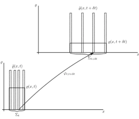
It is worthwhile to mention that one has very similar situation in the case of continuum mechanics. Consider the following simple example. A puff of gas is sprayed into an empty room through a little pipe (Fig. 7). As the gas is spreading, the density of the gas$(x,t)is continuously decreasing in every point of the instantaneous region occupied by the gas (Fig. 8). Consequently,

$(x,t)does not satisfy the equation of persistence. This means that the density distribution, which is one of the basic quantities of the continuum mechanical description of the gas, cannot be in the package of intrinsic properties tracking the gas.

In contrast, assuming that the gas consists of a huge number of small rigid particles, thefine-graineddensity distribution ˜$(x,t) looks like as depicted in Fig. 8 and satisfies the equation of persistence (6) with a suitable local and instantaneous velocity field, the value of which at every point in a region oc- cupied by a particle is equal to the instantaneous velocity of the particle con- cerned. The course-grained density supervenes on the fine-grained density;

Figure 8: The density of the gas$(x,t)is continuously decreasing in every point of the regionΣtoccupied by the gas. Consequently,$(x,t)does not satisfy the equation of persistence. In contrast, the fine-grained density distribution$˜(x,t), reflecting the molecular structure of the gas, does satisfy the equation of persistence

not pointwise, but in the style of (47)–(48):

$(r,t) = ¹ Ω

ˆ

Ωr

˜

$(r,ˆ t)d³(rˆ)

whereΩr denotes a sphere of volumeΩ with centerr, large enough relative to the fine-grained structure, but small enough to have a meaningful smooth approximation.

It is worth noting that while continuum mechanics alone is thus incapable of accounting for the persistence of the gas, the continuum mechanical descrip- tionitself also tacitly assumes that the gas constitutes a persisting entity. The reason is that the continuum mechanical description refers to a velocity field, as one of its fundamental quantities. For example, the coarse-grained density

$(x,t)of the spreading gas obeys a continuity equation

∂t$(r,t) +∇($(r,t)_v(r,t)) =0

expressing that the quantity of the gas remains constant upon spreading out.

Here $(r,t)v(r,t) is the convection current density attached to the local mo- tion of the gas at space-time point(r,t). Nowwhosevelocity is v(r,t)? One might think that within continuum mechanics v(r,t) can be interpreted as the velocity of the local part of a persisting continuum located at rat timet.

However, continuum mechanics itself fails to support such an interpretation:

the coarse-grained quantities featuring the continuum mechanical description, among them$(x,t), fail to satisfy the equations of persistence, as the example of the spreading gas demonstrates, and hencev(r,t)is not definable in terms of the properties of the continuum described by continuum mechanics. It is thus no surprise that this is not the way the fundamental fieldv(r,t)is finally explicated (cf. Truesdell and Toupin p. 227 vs. p. 327). Instead,v(_r,t)_{is expli-} cated by going beyond the domain of the continuum mechanical description,

in terms of the molecular structure of the gas: v(r,t)is defined on the basis of the velocities of the particles of the gas, located aroundrat timet, by means of some averaging procedures (see Murdoch 2012, Section 3.6).

The upshot of all this is that the continuum mechanical description of the gas in terms of the course-grained quantities is ontologically incomplete.

This incomplete description can be completed by appealing to the fine-grained structure of the gas (cf. Murdoch 2012, Chapter 3; Batterman 2006). The per- plexing question is: what could be a similar fine-grained structure of a classical electromagnetic field?

Acknowledgment

The research was partly supported by the (Hungarian) National Research, De- velopment and Innovation Office, No. K100715 and No. K115593.

References

Arntzenius, Frank (2000): Are There Really Instantaneous Velocities? The Monist83, pp. 187–208.

Batterman, Robert W. (2006): Hydrodynamics versus Molecular Dynamics:

Intertheory Relations in Condensed Matter Physics,Philosophy of Science 73, pp. 888-904.

Butterfield, Jeremy (2005): On the Persistence of Particles, Foundations of Physics35, pp. 233–269.

Butterfield, Jeremy (2006): The Rotating Discs Argument Defeated, British Journal for the Philosophy of Science57, pp. 1–45.

Frisch, Mathias 2005: Inconsistency, Asymmetry, and Non-Locality, Oxford: Ox- ford University Press.

Gömöri, Márton and Szabó, László E. (2013): Operational understanding of the covariance of classical electrodynamics, Physics Essays 26, pp.

361–370.

Hawley, Katherine (2001): How Things Persist. Oxford: Oxford University Press.

Heil, John (2003): From an Ontological Point of View. Oxford: Clarendon Press.

Jackson, John D. (1999): Classical Electrodynamics (Third edition). Hoboken, NJ:

John Wiley & Sons.

Kuhlmann, Meinard (2015): Quantum Field Theory, The Stanford Encyclopedia of Philosophy (Summer 2015 Edition), Edward N. Zalta (ed.), URL =

<https://plato.stanford.edu/archives/sum2015/entries/quantum- field-theory/>.

Murdoch, A. Ian (2012): Physical foundations of continuum mechanics. Cam- bridge: Cambridge University Press.

Reichenbach, Hans (1965): The Theory of Relativity and A Priori Knowledge.

Berkeley and Los Angeles: University of California Press.

Sider, Theodore (2001): Four-Dimensionalism. Oxford: Oxford University Press.

Swartz, Norman (1991): Beyond Experience – Metaphysical Theories and Philo- sophical Constraints (Second Edition). Toronto: University of Toronto Press.

Tooley, Michael (1988): In Defense of the Existence of States of Motion,Philo- sophical Topics16, pp. 225–254.

Truesdell, Cifford and R. A. Toupin 1960: The Classical Field Theories. In S.

Flügge (ed.),Encyclopedia of Physics Vol. III.Berlin: Springer.