We investigate these representations of the polycyclic monoids, and we generalize some results from [16]

(1)

ON STRONG AFFINE REPRESENTATIONS OF THE POLYCYCLIC MONOIDS

MIKL ´OS HARTMANN AND TAM ´AS WALDHAUSER

Abstract. Jones and Lawson have discovered in [16] that certain representations of the so-called polycyclic monoids are closely related to some permutative representations of the Cuntz algebrasOnstudied by Bratteli and Jorgensen in [4].

We investigate these representations of the polycyclic monoids, and we generalize some results from [16]. We give a (sharp) upper bound on the number of atoms in case one of the parameters tends to infinity and present an infinite family of representations having only one atom. Furthermore, by making use of a C++

program we present some observations regarding the number of atoms in the case n= 3.

1. Introduction

Letd1, . . . , dn be a complete system of residues modulon(i.e., integers that represent each residue class modulon) and letfi: Z→nZ+di, x7→nx+di. The union of the inverse mapsf_i⁻¹constitutes a transformationR:Z→Zdefined byR(x) =^x−d_n ⁱ, whered_i is the unique element of the setD={d1, . . . , d_n} such thatx≡d_i (modn).

In this paper we investigate the set B_∞(D) of periodic points ofR:

(1.1) B_∞(D) :=

x∈Z:R^`(x) =xfor some`∈N .

Determining the number and structure of periodic orbits of R is a highly nontrivial problem, which is of interest on its own, and it is also connected to the study of representations of the polycyclic monoids and of the Cuntz C^∗-algebras as well as to generalized radix representations and the corresponding “digit tilings” of Euclidean spaces. We briefly describe these connections below, but in the rest of the paper we refer only to the elementary setup outlined above, in order to make the paper more accessible and self-contained.

1.1. Radix representations. Iterating the mapRon a given integerxand recording at each step the element ofD that we used, we obtain a sequencea0, a1, . . .∈D such thatRⁱ(x)≡ai (modn) for everyi∈N0. It is then straightforward to verify thatx= a0+na1+· · ·+n^k−1a_k−1+n^kR^k(x) for allk∈N. Ifx≥0 andD={0,1, . . . , n−1}is the canonical residue system modulon, thenR^k(x) = 0 for sufficiently largek, hence we get x=a0+na1+· · ·+n^k−1ak−1, which is just the usual base-n representation of x. For other choices of D andx, we may not have a finite representation, but we can still regard the formal infinite sum x = a0+na1 +· · ·+n^k−1ak−1+. . . as a generalized n-ary representation of x corresponding to the digit setD. It turns out that the sequence of digits a₀, a₁, . . . is always ultimately periodic, and then one can interpret the infinite radix representation as a geometric series (see Remark 2.10).

Several authors have studied similar, and even more general radix representations:

K´atai and Szab´o [18] considered number systems for Gaussian integers; Gilbert generalized their results to quadratic number fields [11] and also investigated radix representations in arbitrary algebraic number fields [10]. Another widely investigated generalization concerns base-N representations of elements ofZ^ν, whereN is aν×ν

2010Mathematics Subject Classification. 20M18, 20M30, 46L05, 11A63, 37P35.

Key words and phrases. Polycyclic monoids; Cuntz inverse semigroups; affine representations;

Cuntz algebras; permutative representations; atoms of representations; branching function systems;

discrete dynamical systems; periodic points; Cantor set; fractals; radix representations; self-affine tiles.

1

(2)

expanding integer matrix (i.e., every eigenvalue ofN has absolute value greater than one) and the setD of “digits” is a system of representatives of the cosets corresponding to the subgroupNZ^ν ofZ^ν. We refer the reader to the survey paper by Vince [30]

and the references therein for more information on this topic.

1.2. Fractals, tilings and wavelets. Radix representations are closely related to tilings and self-affine sets, which in turn have applications in the theory of wavelets.

First, let us consider once more the standard n-ary number system with digit set D ={0,1, . . . , n−1}, this time considering x∈Rinstead ofx∈Z. If x≥0, thenx has a (possibly infinite and possibly not unique) base-nexpansion x=n^kak+· · ·+ a0+n⁻¹a₋₁+. . . withai∈D. Numbers having no digits to the left of the “decimal”

point (i.e.,ai= 0 for alli≥0) form the interval [0,1], whereas numbers with no digits to the right of the “decimal” point (i.e.,ai = 0 for alli <0) constitute the setN0of nonnegative integers. The subgroup of Rgenerated by N0 is the latticeZ, and it is clear thatRis the union of translates of [0,1] by elements ofZ; moreover, any two of these translated intervals intersect only in a set of measure zero (in fact, in at most one point), i.e., [0; 1] tiles R.

Now if D = {d1, . . . , d_n} is an arbitrary complete system of residues modulo n, then the interval [0,1] shall be replaced by the set

(1.2) T(D) :=

^∞ X

i=1

n⁻ⁱa_i:a_i∈D

.

(This set depends on D as well as on n, but n shall always be clear from the context, and we will sometimes also omit D from the notation when there is no risk of ambiguity.) Note thatTis a self-affine set (a union of smaller copies of itself):

T= d₁ n +1

n·T ∪ · · · ∪ d_n n + 1

n·T.

Bandt [2] proved that T is a compact set with nonempty interior, and Lagarias and Wang [24] showed that the boundary ofThas measure zero. This implies thatTis Jor- dan measurable, and Gr¨ochening and Haas [13] determined its (Jordan or Lebesgue) measure:

(1.3) µ(T) = gcd{di−dj: 1≤i, j≤n}.

Again, T yields a tiling of R (hence the notation T), but this time we need to use translates by the latticeµ(T)·Z(translates byZwould give aµ(T)-fold covering of R) [13, 22, 24].

Similar tiling phenomena occur in the ν-dimensional case outlined in the previous subsection (see, e.g., [23, 22, 24, 30]); in this case we do not have a simple formula for the measure of the corresponding tile T, but Bondarenko and Kravchenko provided an algorithm to compute µ(T) [3]. The tileT is again a self-affine set, often with a fractal structure, and its topological and geometrical properties have been studied by many authors [1, 2, 8, 14, 20]. Gr¨ochenig and Madych [12] established a one-to-one correspondence between certain wavelet bases ofL²(R^ν) and tilesTofR^ν of measure one. Further results relating tilings and wavelets can be found in [7, 21].

1.3. Operator algebras. TheCuntz C^∗-algebraOn isthe C^∗-algebra generated by n pairwise orthogonal isometries on a Hilbert space. More precisely, let H be an infinite-dimensional separable Hilbert space, and let Si(i= 1, . . . , n) be bounded lin- ear operators on H such that S_i^∗Si = I for every i and S1S₁^∗ +· · ·+SnS_n^∗ = I.

This implies that S_i^∗Sj = 0 wheneveri 6=j, and Cuntz [5] has proven that the C^∗- algebra On generated byS1, . . . , Sn is (up to isomorphism) independent of the choice of these isometries – hence the definite article in the first sentence of this paragraph.

The so-called permutative representations of On are defined by Siej =ef_i(j), where {ej:j∈Z}is an orthonormal basis ofH. Thus, in this case the isometriesSipermute the elements of the orthonormal basis. These operators satisfy the defining relations of On if and only if each f_i is injective and their ranges form a partition of Z. In

(3)

particular, the mapsf_i(x) =nx+d_i (i= 1, . . . , n) yield permutative representations of O_n whend₁, . . . , d_n be a complete system of residues modulon. Bratteli and Jor- gensen [4] have studied such representations and their relationship to the dynamics of the mapRand to the structure of the tileT, also in theν-dimensional case mentioned in Subsection 1.1 (we borrow some notation from this paper, in particular, the symbol B_∞ for the set of periodic points). Let us recall a proposition from [4] that will play a crucial rule in Section 6.

Proposition 1.1 ([4]). If D is a complete system of residues modulo n, then the negatives of the integers in T(D) are exactly the periodic points of R: B_∞(D) =

−T(D)∩Z.

Jeong [15] generalized results of [4] about irreducible subrepresentations of permutative representations and obtained an upper bound for the number of periodic points as well as a sufficient condition for R to have only one periodic point. Continued fractions can be regarded as a “base-∞” number system, where the set of digits is N. Kawamura, Hayashi and Lascu [19] adopted this point of view to explore a connection between continued fractions and permutative representations of O_∞; here quadratic irrationals correspond to periodic points.

1.4. Semigroups. For each n≥2 thepolycyclic monoid P_n is defined as a monoid with zero by the presentation

P_n=ha₁, . . . , a_n, a⁻¹₁ , . . . , a⁻¹_n :a⁻¹_i a_i= 1 anda⁻¹_i a_j= 0, i6=ji.

These monoids were introduced by Nivat and Perrot in [29] and have been rediscov- ered by Cuntz [5], hence they are sometimes referred to as the Cuntz inverse semigroups. Besides the Cuntz algebras, the monoidsPnare also related to the Thompson groupsV_n,1[25, 26] and pushdown automata [17]. The important role played by these monoids within semigroup theory is underlined by a result of Meakin and Sapir [28]

showing that congruences of free monoids correspond to certain submonoids of polycyclic monoids (this was generalized to right congruences in [27]), which allows one to translate general questions about monoids to questions about submonoids of polycyclic monoids.

ArepresentationofPnis a monoid homomorphism fromPnto a symmetric inverse monoid, i.e., to the monoid of all partial bijections on a setX. All such representations can be constructed in the following way. LetXbe an infinite set and letX1, . . . , Xn, Y be disjoint subsets ofX such that their union isX and the subsetsXihave the same cardinality as X. For every 1≤i≤n, let fi:X →Xi be a bijection which we will consider to be a partial bijection onX. In this case we can define a representation of Pn by sendingaito fi anda⁻¹_i tof_i⁻¹. IfY =∅then we say that the representation is strong[26]. Thus a strong representation can be given by the data (X;f1, . . . , fn), which is called abranching function system [4]. The strong representations given by (X;f1, . . . , fn) and X˜; ˜f1, . . . ,f˜n

are equivalent if there is a bijection ϕ: X → X˜ such that f_iϕ=ϕf˜_i fori= 1, . . . , n.

Lawson [27] described representations of the polycyclic monoids in terms of strong ones, hence it suffices to study strong representations. Affine representations constitute an important class of strong representations. These are given by X =Z^ν and fi(x) =Nx+di, whereN is a nonsingularν×ν matrix over Zandd1, . . . ,dn is a system of representatives of the cosets corresponding to the subgroupNZ^ν ofZ^ν (cf.

Subsections 1.1 and 1.2). Heren= [Z^ν: NZ^ν] equals the determinant ofN.

In this paper we consider only one-dimensional affine representations, i.e., the case ν = 1. As we shall see, even this seemingly simple case raises highly nontrivial problems, and we are still very far from a full understanding of the one-dimensional strong affine representations of Pn. In the remainder of this section we review some results from the literature that are specific to this one-dimensional case, and we briefly and informally explain our contributions to this topic.

(4)

1.5. Main results. The structure of the one-dimensional strong affine representation of P_n corresponding to (Z;f₁, . . . , f_n) withf_i(x) =nx+d_i, whereD={d₁, . . . , d_n} is a complete system of residues modulon, is to a large extent determined by the set B_∞(D) of periodic points (see Section 2 for more details). Bandt [2] already mentions that R has only a finite number of periodic orbits and hints at the importance of studying these orbits in connection with radix representations and tilings, and several authors considered sporadic examples, mainly for n = 3 (see, e.g., [4, 12, 30]). Let us also mention the recent paper by Dutkay and Haussermann [6] where the case n= 4, D ={0, m} with mbeing an odd integer is analyzed. Clearly, here D is not a complete system of residues modulon(hence the mapR is only partially defined), but the periodic orbits ofRstill have interesting number-theoretic properties and they have relevance to the harmonic analysis of a certain fractal measure.

Our work is motivated by the papers [4] and [16], which appear to contain the only systematic studies of the periodic points, namely, for n = 2. In this case one can assume without loss of generality thatD={0, p}, wherepis an odd positive integer (see Fact 2.2). Bratteli and Jorgensen [4] proved thatB_∞(0, p) ={−p, . . . ,−1,0}and that the period of an arbitraryx∈B_∞(0, p) equals the order of 2 modulop/gcd (x, p).

It is well known (and a nice exercise in number theory) that this order is the same as the period of the binary expansion of the fractionx/p. Jones and Lawson [16] showed that this is not a coincidence: the structure of the cycle containing x is strongly related to the digits in the binary expansion ofx/p. Two other special cases are also considered in [4], namely,B_∞(0,1, . . . , n−1) ={−1,0}andB_∞(1,3,5) ={−2,−1}.

In all of the special cases mentioned above,d1, . . . , dnis an arithmetic sequence. In Section 3 we generalize the results of [4, 16] by proving that the setB_∞(D) consists of the integers in the interval I :=

−_n−1^dⁿ ,−_n−1^d¹

wheneverd₁, . . . , d_n is an arithmetic sequence (Theorem 3.1), and we also relate the structure of the cycle containing the integer x∈B_∞(D) to the n-ary expansion of the fraction ^(n−1)x+d_d ¹

n−d1 (Theorem 3.3).

It is easy to see that we have B_∞(D) ⊆ I for every D (Fact 2.4), hence we can say that for arithmetic sequences the set of periodic points is as large as possible.

We show in Section 4 that we may have such a large set of periodic points even if d1, . . . , dnis not an arithmetic sequence. We will characterize explicitly the sequences satisfying B_∞(D) =I ∩Z (Theorem 4.1), and we will see that these sequences are in some sense not far from being arithmetic (Remark 4.2). In Section 6 we study the asymptotic behaviour of the number of periodic points as one of the parameters, say d_n, tends to infinity, whiled₁, . . . , d_n−1are fixed. We prove that|B∞(D)|=O d^logn ⁿ² (Theorem 6.4), and we also provide infinite series of examples showing that this upper bound cannot be improved (Theorem 6.5). For a lower bound, we have the trivial estimate|B_∞(D)| ≥1, and we will prove in Section 5 that in general one cannot have a better lower bound, since it is possible to letd_n tend to infinity in such a way that the number of periodic points stays constant 1 (Theorem 5.1).

2. Preliminaries

We recall some facts from [4, 16, 27] that we shall need in the sequel; we present these in terms of branching functions systems, which provide a combinatorial frame- work for studying permutative representations of the CuntzC^∗-algebrasOnand strong representations of the polycyclic monoidsPn, hence familiarity with the theory of operator algebras or semigroups is not assumed.

Abranching function systemis a tuple (X;f1, . . . , fn), whereXis an infinite set and fi: X →X(i= 1, . . . , n) are injective maps such that their ranges form a partition ofX. One can visualize a branching function system as a directed graph with colored edges: the vertices are the elements of X, and an arrow of coloriis drawn fromxto y iffi(x) =y; we shall frequently refer to this graph in the following. We say that two branching function systems areequivalent if the corresponding colored graphs are isomorphic (where the isomorphism is required to preserve colors); this corresponds to the usual notion of equivalence of representations of semigroups.

(5)

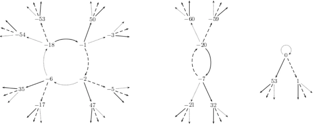
Figure 1. A part of the graph of the branching function system with parameters (d1, d2, d3) = (0,1,53)

Observe that the definition of a branching function system requires that for every vertex there are noutgoing edges (one of each of the ncolors, leading to ndifferent vertices) and that there is exactly one incoming edge. These two properties imply that there can be at most one cycle in every connected component of the graph and this cycle must be directed. (By a cycle we mean a closed path, as usual in graph theory.

However, note that this terminology is different from that of [4, 16]; see Remark 2.1.) It is straightforward to verify that if a connected component contains a cycle, then the order of the colors appearing in the cycle determine that connected component up to isomorphism. (See Figure 1; it shows only a finite part of the graph of a branching function system with n = 3, but the missing parts are easy to imagine: an infinite ternary tree is rooted at the vertices −54,−53,50,−3, etc. The numbering of the vertices will be explained later.) Let us note that cycle-free components can be more complicated; however, for the special branching function systems that we consider in this paper, each component contains a cycle (see Fact 2.4).

The inverses of the maps f_i are partial bijections onX whose union is a surjective map R:X →X, whereR(x) is the unique elementy ∈X such that there existsi∈ {1, . . . , n}withf_i(y) =x. The branching function system (X;f₁, . . . , f_n) can also be studied via the discrete dynamical system (X;R). Thetrajectory x, R(x), R²(x), . . . of a point x can be seen as a walk in the graph that starts from x and follows the arrows backwards. Letσ(x) = (j0, j1, . . .) be the sequence of the colors of the edges in this walk: x=fj₀(R(x)),R(x) =fj₁ R²(x)

, etc.; this defines the so-called coding map σ:X → {1, . . . , n}^N⁰. We say thatxis aperiodic point if the trajectory of xis periodic, i.e., if xis a fixed point of R^`(x) for some `∈ N. If ` is the least positive exponent such that R^`(x) = x, then (and only then) x lies on a cycle of length ` in the graph. Following [4], we denote the set of periodic points by B_∞. Using the terminology of discrete dynamical systems, we shall say that a setA⊆X ispositively invariant ifR(A)⊆A, andAis said to beabsorbingif for everyx∈X, the trajectory ofxlies eventually inA, i.e., we have

R^t(x), R^t+1(x), . . . ⊆Afor somet∈N. Remark 2.1. Let us define two equivalence relations ∼and ≈onX byx∼y ⇐⇒

∃s, t:R^s(x) =R^t(y) andx≈y ⇐⇒ ∃t:R^t(x) =R^t(y). In [4, 16] the main objects of study are the blocks of∼and≈, which were called there cycles and atoms, respectively. Our terminology is different: we use the term cycle in the graph-theoretical sense, and we refer to the blocks of∼as connected components. For branching function systems corresponding to one-dimensional affine representations of P_n, there is a one-to-one correspondence between atoms and periodic points (see Scholium 3.9 of [4] and Proposition 4.9 of [16]). Since we deal only with this case, we work with the simpler concept of a periodic point instead of that of an atom.

Now let us turn to the special branching function systems mentioned in Subec- tion 1.5. The notation that we introduce here will be used throughout the paper

(6)

without further mention. Let n ≥ 2 be a positive integer, let D ={d1, . . . , d_n} be a complete system of residues modulo n, and letq_i and r_i denote the quotient and the remainder of d_i, when divided by n, i.e., d_i =nq_i+r_i and 0≤r_i < n. Clearly, we have {r₁, . . . , r_n} ={0, . . . , n−1}. The functions f_i(x) :=nx+d_i(i= 1, . . . , n) define a branching function system (Z;f1, . . . , fn), and the corresponding dynamical system is (Z;R), whereR(x) = ^x−d_nⁱ withdi being the uniqe element of Dsuch that x≡di (modn). As an example, see Figure 1, which shows the graph of the branching function system corresponding to n = 3 and (d1, d2, d3) = (0,1,53), where dotted, dashed and solid arrows represent f1, f2 and f3, respectively. Iterations ofR can be seen in the figure by following the arrows backwards. For instance, the trajectory of 50 is 50,−1,−18,−6,−2,−1,−18,−6,−2, . . .andσ(50) = (3,3,1,1,2,3,1,1,2, . . .).

In the following we collect some basic facts about these branching function systems.

These results all appeared in [4, 16, 27]; for the reader’s convenience we restate and reprove them. Unless otherwise mentioned, we will always assume thatd₁<· · ·< d_n. Fact 2.2. The following sequences give rise to equivalent branching function systems:

a) d₁, . . . , d_n;

b) −d₁,−d₂, . . . ,−d_n;

c) d1+k(n−1), d2+k(n−1), . . . , dn+k(n−1), for arbitraryk∈Z.

Proof. It is easy to check that the mapsβ:Z→Z, x7→ −xandγ:Z→Z, x7→x−k establish isomorphisms from the graph corresponding to a) to the graph corresponding

to b) and c), respectively.

By this fact, one can always assume that the parameters d1<· · ·< dn are chosen such that 0≤d1< n−1. LetI denote the interval

−_n−1^dⁿ ,−_n−1^d¹

, letA(D) =I ∩Z and let B_∞(D) be the set of periodic points, as defined in (1.1); sometimes we will write simplyAandB_∞whenever the parametersd1, . . . , dnare clear from the context.

(From Figure 1 we see thatB∞(0,1,53) ={−20,−18,−7,−6,−2,−1,0}and we have A(0,1,53) ={−26, . . . ,0}.)

Lemma 2.3. The setA is a finite positively invariant absorbing set.

Proof. Since d₁ <· · · < d_n, we have ^x−d_nⁿ ≤R(x)≤ ^x−d_n¹ for every x∈ Z. From these inequalities one can deduce the following implications:

a) x < −dn

n−1 =⇒ x < R(x) < −d1

n−1; b) −dn

n−1 ≤ x ≤ −d1

n−1 =⇒ −dn

n−1 ≤ R(x) ≤ −d1

n−1; c) −d₁

n−1 < x =⇒ −d_n

n−1 < R(x) < x.

The second implication immediately yields thatAis positively invariant. Ifx /∈ A then either x < R(x) < R²(x) <· · · < R^t(x)∈ Aor x > R(x) > R²(x) >· · · >

R^t(x)∈ Afor somet∈Nby a) or c) depending on whetherx <−_n−1^dⁿ orx >−_n−1^d¹ . In both cases b) shows that the rest of the trajectory of xstays inA.

Fact 2.4. The graph corresponding to the branching function system determined byD has finitely many connected components, and each component contains a cycle. These cycles are all contained in A(D), i.e., we have

B∞(D)⊆ A(D).

The trajectory of every integer x∈Z is eventually periodic: there exist `, t∈N such that R^i+`(x) =Rⁱ(x) wheneveri≥t.

Proof. For every x ∈ Z, the trajectory of x is finite, since Rⁱ(x) belongs to the finite set A for almost everyi, by Lemma 2.3. This implies that every trajectory is eventually periodic, hence each connected component contains a cycle. These cycles are contained in A, thus there are finitely many cycles and finitely many connected

components.

(7)

According to Fact 2.4, B_∞ is a nonempty set consisting of finitely many cycles, and every trajectory eventually winds around one of these cycles. This implies that the sequenceσ(x) is also eventually periodic for everyx∈Z. We show below how to use these facts to see that σ(x) uniquely determinesx, i.e., that the coding map is injective. (Representations ofOnwith an injective coding map are called multiplicity- free representations in [4].)

Fact 2.5. Suppose that the trajectory of x becomes `-periodic after t terms, i.e., R^t+`(x) =R^t(x), and letσ(x) = (j0, j1, . . .). Then we have

(2.1) x=dj₀+ndj₁+· · ·+n^t−1djt−1−dj_tn^t+· · ·+djt+`−1n^t+`−1

n^`−1 .

Proof. From the definition of R and σ one can deduce by induction on k that x = dj₀+ndj₁+· · ·+n^k−1djk−1+n^kR^k(x) holds for allk∈N. Applying this formula for k=tandk=t+`we obtain

x=dj₀+ndj₁+· · ·+n^t−1djt−1+n^tR^t(x)

=d_j₀+nd_j₁+· · ·+n^t−1d_j_t−1+n^td_j_t+· · ·+n^t+`−1d_j_t+`−1+n^t+`R^t+`(x). By our assumption we haveR^t+`(x) =R^t(x), hence 1−n^`

n^tR^t(x) =n^tdj_t+· · ·+

n^t+`−1d_j_t+`−1 follows, and this proves (2.1).

If x ∈ B_∞ lies on a cycle of length `, then the sequence σ(x) is `-periodic, that is, σ(x) = (j₀, . . . , j_`−1, j₀, . . . , j_`−1, . . .), so we can describe it by a finite word w =j₀· · ·j_`−1 over the alphabet {1, . . . , n}, which we will refer to as the word corresponding to x. This word can be read from the graph by recording the colors of the edges on the cycle, starting from xand following the arrows backwards. Words corresponding to periodic points on the same cycle are conjugates, i.e., they can be obtained from each other by cyclic shifts. (For example, the words corresponding to

−1,−2,−6 and−18 on Figure 1 are 3112, 2311, 1231 and 1123, respectively.) Since our branching function systems have finitely many connected components, each containing a cycle (see Fact 2.4), their structure can be completely described by the words corresponding to periodic points (or cycles). Therefore, exploring periodic points and the corresponding words is essential in the study of representations of Pn andOn.

If a wordwis not the repetition of a shorter word, i.e., it cannot be written in the form w=u· · ·u=u^k(k≥2), then w is said to be a primitive word. Observe that every word is the power of a unique primitve word. The next corollary of Fact 2.5 states that the word corresponding to a periodic point is always primitive, and we also get a characterization of those primitive words that correspond to a periodic point.

(Note that primitivity of the word corresponding toxmeans that the shortest period of σ(x) is the same as he shortest period of the sequencex, R(x), R²(x), . . .. In an arbitrary branching function system it is possible that the former is a proper divisor of the latter; however, this cannot happen for the special branching function systems considered here.)

Corollary 2.6. A word w=j0· · ·j`−1 over{1, . . . , n} corresponds to some periodic point if and only if wis primitive and

(2.2) x=−dj`−1n^`−1+· · ·+dj₁n+dj₀

n^`−1

is an integer. If this holds, then the integer x defined by (2.2)is a periodic point on a cycle of length `, andw is the word corresponding tox.

Proof. First we prove the second statement: let us assume that w= j0· · ·j_`−1 is a primitive word such that the number given by (2.2) is an integer. Thenx=dj₀+dj₁n+

· · ·+d_j_`−1n^`−1+n^`x, which implies thatR(x) =^x−d_n^j⁰ =d_j₁+· · ·+d_j_`−1n^`−2+n^`−1x, sincex≡dj₀ (modn), anddj₀ is the only element ofDwith this property. Continuing this way we get R²(x) = ^R(x)−d_n ^j¹ =dj₂+· · ·+dj_`−1n^`−3+n^`−2x, etc., and after ` steps we obtainR^`(x) =x. This means thatxis indeed a periodic point; furthermore,

(8)

if uis the word corresponding toxthenw=u^k with` =km, where mdenotes the length of u (that is, the length of the cycle that containsx). Sincew is a primitive word, we must havek= 1, thus the length of the cycle containingxis`and the word corresponding to xisw.

The argument above proves not only the second statement of the corollary, but also the “if” part of the first statement, thus it remains to prove the “only if” part. Let w = j0· · ·j_`−1 be the word corresponding to some periodic point y. We can apply Fact 2.5 with t = 0 to obtain that the right hand side of the equality (2.2) equals y, therefore it is an integer. Finally, we prove primitivity of w: let w = u^k, where u=j0· · ·jm is a primitive word and` =km. Then we haveji =jimodm for every i∈ {0, . . . , `−1}, and this allows us to rewrite the right hand side of (2.2) as follows:

x=− d_j_m−1n^m−1+· · ·+d_j₁n+d_j₀

· 1 +n^m+· · ·+n^(k−1)m n^`−1

=− djm−1n^m−1+· · ·+dj1n+dj0

·ⁿ_n^kmm−1⁻¹

n^`−1 =−djm−1n^m−1+· · ·+dj₁n+dj₀

n^m−1 .

Applying the first paragraph of this proof to the primitive word u, we see that x belongs to a cycle of lengthm(and the word corresponding toxisu). Consequently,

k= 1 andu=w, proving thatwis indeed primitive.

Remark 2.7. The proof of Corollary 2.6 shows that if the numberxgiven by (2.2) is an integer, then it is a periodic point even if the wordw is not primitive. Moreover, ifw=u^k, whereuis a primitive word, then the word corresponding toxisu. Thus, the periodic points are exactly the integers of the form

a_`−1n^`−1+· · ·+a1n+a0

1−n^` (`∈N, a₀, . . . , a_`−1∈D).

Two such expressions yield the same number if and only if the words describing the coefficients a0, . . . , a`−1 are the powers of the same primitive word. In particular, different expressions of the same length`give different periodic points.

Fact 2.8. The words corresponding to periodic points on different cycles are not con- jugate.

Proof. Let v and w be words corresponding to periodic points x and y that lie on different cycles, and suppose thatvandware conjugates. Then there exists a pointx⁰ on the same cycle asxsuch that the word corresponding tox⁰isw. However, according to Corollary 2.6, a periodic point is uniquely determined by the corresponding word by (2.2). This implies thatx⁰=y, hencexandy belong to the same cycle, contrary

to our assumption.

Summarizing the above facts, we can say that the structure of the branching function system corresponding tod1, . . . , dnis determined by a finite set of primitive words over the alphabet{1, . . . , n}, each considered up to conjugacy. For the sake of canon- icity, it is customary to choose the lexicographically least word from each conjugacy class; these words are called Lyndon words. (The Lyndon words describing the three cycles of Figure 1 are 1123, 23 and 1.) One possible approach to find these Lyndon words is to follow the trajectories of the elements of A(D). Another possibility is to determine all numbers of the form a`−1n^`−1+· · ·+a1n+a0 with a0, . . . , a`−1∈ D that are divisible byn^`−1 (cf. Remark 2.7). SinceA(D) is finite, both searches can be completed in a finite number of steps (note that we must have`≤ |B∞| ≤ |A|).

Corollary 2.9. It is decidable whether two one-dimensional strong affine representations of P_n are equivalent.

Remark 2.10. Letσ(x) = (j₀, j₁, . . .) and let us write out the representations ofx considered in the proof of Fact 2.5 fork= 1,2,3, . . .:

x=d_j₀+nR(x) =d_j₀+nd_j₁+n²R²(x) =d_j₀+nd_j₁+n²d_j₂+n³R³(x) =· · · .

(9)

It would be natural to extend this to an infinite expansion ofx:

(2.3) x=d_j₀+nd_j₁+n²d_j₂+n³d_j₃+· · · .

Of course, this infinite series does not converge in general. However, we can infer from (2.3) thatx≡d_j₀ (modn),x≡d_j₀+nd_j₁ modn²

,x≡d_j₀+nd_j₁+n²d_j₂ modn³ , etc. Moreover, since the expansion is periodic, we can sum the right hand side of (2.3) formally by letting 1 +n^`+n^2`+· · ·= _1−n¹ _`. Although this geometric series is clearly divergent, this formal evaluation gives actually the correct value of x. Indeed, let a=dj₀+ndj₁+· · ·+n^t−1djt−1andb=dj_tn^t+· · ·+djt+`−1n^t+`−1(withtand`being the same as in Fact 2.5); then we can rewrite (2.3) asx=a+b+bn^`+bn^2`+· · ·=a+_1−n^b _`, and this is the same as (2.1).

One can regard (2.3) as a representation ofxin a number system with radixnand digitsd1, . . . , dn. As mentioned in Subection 1.5,B∞(0, . . . , n−1) ={−1,0}(see also Theorem 3.1). This means that using the standard digits 0, . . . , n−1, the sequence of digits in the expansion of every integer is eventually constant 0 or constantn−1, namely for nonnegative integers the digits are eventually 0 (as it is well known), and for negative integers the digits are eventuallyn−1. For instance, the representation of x=−1 is−1 = (n−1) + (n−1)n+ (n−1)n²+· · ·, which can be verfied using the formal summation 1 +n+n²+· · ·= _1−n¹ .

As another example, we can read from Figure 1 that 50 can be represented in the number system with radix 3 and digits 0,1,53 as

50 =d₃+nd₃+n²d₁+n³d₁+n⁴d₂+n⁵d₃+n⁶d₁+n⁷d₁+n⁸d₂+· · ·

= 53 + 53·3 + 0·3²+ 0·3³+ 1·3⁴+ 53·3⁵+ 0·3⁶+ 0·3⁷+ 1·3⁸+· · ·

= 53 + 240· 1 + 3⁴+ 3⁸+· · · .

Evaluating 1+3⁴+3⁸+· · · formally as₁₋₃¹4, we indeed get 53+240·₋₈₀¹ = 53−3 = 50.

Finally, we state an elementary identity about integer parts that will be needed later; its proof is left to the reader.

Lemma 2.11. For allx∈Randn∈Nwe havePn−1 k=0

x+^k_n

=bnxc.

3. Arithmetic sequences

In this section we investigate periodic points and cycles in the case when the parameters form an arithmetic sequence. For notational convenience, we shift the indices by 1 (as it is done in Section 5 of [16]): instead ofd₁, . . . , d_nwe shall work withd₀, . . . , d_n−1, and we will use words over {0, . . . , n−1} to describe the cycles. Thus, we assume throughout this section that d0, . . . , d_n−1 is an arithmetic sequence: di=d0+ihfor i = 0, . . . , n−1, whereh∈Nis relatively prime ton and 0≤d0< n−1. Observe that A={−h, . . . ,−1,0}ifd0= 0 andA={−h, . . . ,−1}if 0< d0< n−1.

Theorem 3.1. Ifd0<· · ·< dn−1 is an arithmetic sequence, thenB∞=A, therefore the number of periodic points is h+ 1 orh(depending on whether d0= 0 or not).

Proof. Since Ais a positively invariant set (Lemma 2.3) and B_∞ ⊆ A(Fact 2.4), it suffices to prove that the restriction of R toA is bijective. In fact, it is sufficient to establish injectivity, as A is finite. Letx, y, z ∈ A such thatR(x) =R(y) =z and x < y. Then we have x=nz+di, y =nz+dj for some i, j ∈ {1, . . . , n}, therefore y−x=dj−di=h(j−i)≥h. If d06= 0 then this is already a contradiction, as the diameter of the setAish−1 in this case. Ifd0= 0, then the diameter ofAish, and this implies that x= minA=−handy = maxA= 0. However,R(−h) = −hand R(0) = 0, contradicting the assumption R(x) =R(y).

The next lemma is essentially just a reformulation of Corollary 2.6 for arithmetic sequences.

(10)

Lemma 3.2. Assume that the sequence d₀ < · · · < d_n−1 is arithmetic, let w = j₀· · ·j_`−1 be a primitive word over {0, . . . , n−1} and let ←w− ∈

0,1, . . . , n^`−1 be the nonnegative integer given by the base-n representation determined by the reverse of w:

←w−=j_`−1· · ·j1j0n=

`−1

X

i=0

jinⁱ.

Thenw corresponds to a cycle if and only if n^`−1

d0(n^`−1)

n−1 +h←w .−

Proof. Substitutingd0+jihfordj_i in the numerator of the right hand side of (2.2),we obtain

`−1

X

i=0

d₀nⁱ+

`−1

X

i=0

j_ihnⁱ= d₀(n^`−1) n−1 +h←w .−

By Corollary 2.6, w corresponds to a periodic point if and only if the above number

is divisible by n^`−1.

Now we are ready to generalize Theorem 5.5 of [16] by relating the words corresponding to periodic points to base-nexpansions of certain fractions. (Note that for n= 2 we must haved0= 0, hence the following theorem indeed contains Theorem 5.5 of [16] as a special case.)

Theorem 3.3. Assume that d₀ < · · · < d_n−1 is an arithmetic sequence. If d₀ = 0 then the words corresponding to the periodic points are the reverses of the periods of the base-n representations of the fractions _h⁰, . . . ,^h_h. If 0 < d₀ < n−1, then the corresponding words are the reverses of the periods of the base-n representations of

1

h−_h(n−1)^d⁰ , . . . ,^h_h−_h(n−1)^d⁰ .

Proof. Let x∈ B∞ and let w =j0· · ·j`−1 be a primitive word over {0, . . . , n−1}.

By (the proof of) Lemma 3.2, w corresponds to x if and only if−x= _n−1^d⁰ + _n^h_`^←₋₁^w⁻ , which is equivalent to

−x+_n−1^d⁰

h =

←w /n− ^` 1−1/n^` =←w−

1 n^` + 1

n^2` +· · ·

=j`−1

1

n+· · ·+j0

1 n^` +j`−1

1

n^`+1 +· · ·+j0

1 n^2` +· · ·

= 0. j`−1· · ·j0j`−1· · ·j0· · ·n.

Thus, the word corresponding to x∈B∞ is the reverse of the period in the base-n expansion of−_h^x−_h(n−1)^d⁰ . Taking into account thatB∞={−h, . . . ,−1,0} ifd0= 0 and B_∞={−h, . . . ,−1}if 0< d0< n−1, we obtain the (negatives of the) fractions

listed in the statement of the theorem.

Corollary 3.4. IfD is an arithmetic sequence, then the length of the cycle containig the periodic point

x∈B_∞(D)

equals the multiplicative order of nmodulo ^h(n−1)

gcd x(n−1)+d0,h(n−1).

Proof. It is well known that if a, b ∈ N are relatively prime and b is also relatively prime ton, then the length of the period of the base-nrepresentation of ^a_b is the order ofnmodulob. We have seen in the proof of Theorem 3.3 that the length of the cycle containing x∈B∞ is the length of the period of the base-nexpansion of ^x(n−1)+d_h(n−1)⁰; therefore, it only remains to observe that after simplification the denominator becomes

h(n−1)

gcd x(n−1)+d0,h(n−1), which is clearly relatively prime to n, as both h and n−1

are.

(11)

Corollary 3.5. For any finite setC of primitive words over the alphabet{0, . . . , n− 1} there exists an arithmetic sequence d₀ < · · · < d_n−1 such that the set of words corresponding to the elements of B_∞(d₀, . . . , d_n−1)containsC.

Proof. By Lemma 3.2, it suffices to findd0 andhsuch that d₀(n^|w|−1)

n−1 +h←w−≡0

modn^|w|−1

for every w ∈ C, where |w| denotes the length of w. Clearly, for d0 = 0 and h = lcm

n^|w|−1 :w∈C each of these congruences are satisfied (note thathis relatively

prime ton).

We finish this section by showing that the only equivalences between representations (or branching function systems) given by arithmetic sequences are the trivial ones of Fact 2.2.

Theorem 3.6. Let 0 ≤ d₀, d⁰₀ < n−1 and let h, h⁰ be relatively prime to n. The representations ofPnarising from the arithmetic sequencesd₀, d₀+h, . . . , d₀+(n−1)h andd⁰₀, d⁰₀+h⁰, . . . , d⁰₀+ (n−1)h⁰ are equivalent if and only ifd₀=d⁰₀ andh=h⁰. Proof. Let the two representations given in the statement of the theorem be equivalent, and first let us assume that h6= h⁰; without loss of generality we can suppose that h < h⁰. Since equivalent representations have the same number of periodic points, Theorem 3.1 implies that d₀= 0, d⁰₀6= 0 and h⁰ =h+ 1. Then 0∈B_∞(d₀, . . . , d_n−1) and the corresponding word is 0 (of length one). However, since n−1-d⁰₀, this word corresponds to no element of B_∞ d⁰₀, . . . , d⁰_n−1

, contradicting the equivalence of the representations.

Now let us assume that h=h⁰ but d0 6=d⁰₀. Recall that two representations are equivalent if and only if the sets of words determined by their periodic points are the same. Letwbe a word of length`corresponding to some element ofB_∞(d0, . . . , d_n−1);

then w also corresponds to some element of B_∞ d⁰₀, . . . , d⁰_n−1

. Lemma 3.2 implies that

d0(n^`−1)

n−1 +h←w−≡d⁰₀(n^`−1)

n−1 +h⁰←w−≡0 modn^`−1 ,

which in turn implies thatd0≡d⁰₀ (modn−1), ash=h⁰. However, this is impossible,

since 0≤d₀, d⁰₀< n−1 andd₀6=d⁰₀.

4. Many periodic points

Arithmetic sequences give rise to branching function systems where the set of periodic points is “as large as possible”, i.e., B_∞ =A. In this section we characterize sequences d1, . . . , dn that have the same property; as we shall see, these are “almost arithmetic sequences”.

Theorem 4.1. Letd1<· · ·< dn, letI denote the interval

−_n−1^dⁿ ,−_n−1^d¹

as before, and letIi=_n¹I −_n¹d_i fori= 1, . . . , n. The following conditions are equivalent:

(i) B_∞=A;

(ii) A ⊆ I1∪ · · · ∪ In;

(iii) for all i∈ {1, . . . , n−1} we have d₁

n(n−1)+d_i+1 n

= d_n

n(n−1) +d_i n

.

Proof. Just as in the proof of Theorem 3.1, we can see that B_∞ =A if and only if the restriction of R to A is bijective. Since A is finite, bijectivity is equivalent to surjectivity in this case, thus (i) holds if and only if R⁻¹(x)∩ A=R⁻¹(x)∩ I 6=∅ for all x ∈ A. This latter condition means that for every x ∈ A there exists an i ∈ {1, . . . , n} such thatnx+di ∈ I, i.e., x∈ Ii. This proves the equivalence of (i) and (ii).

The intervals Ii are all translates of the interval _n¹I. The leftmost one of these intervals is In, and the left endpoint of In coincides with the left endpoint of I;

(12)

similarly, the right endpoint ofI1 coincides with the right endpoint of I. Therefore, condition (ii) holds if and only if there is no integer between the right endpoint of I_i+1 and the left endpoint ofI_i for everyi∈ {1, . . . , n−1}:

(4.1) @x∈Z: − d1

n(n−1)−di+1

n < x <− dn

n(n−1)−di

n.

Since 16=i+ 1, we haved₁ 6≡d_i+1 (modn), and this implies that −_n(n−1)^d¹ −^dⁱ⁺¹_n is not an integer; similarly, the right hand side of (4.1) is not an integer either, asn6=i.

Hence (4.1) is equivalent to j

−_n(n−1)^d¹ −^dⁱ⁺¹_n k

≥j

−_n(n−1)^dⁿ −^d_nⁱk

, which, in turn, is equivalent to

(4.2)

d1

n(n−1)+di+1

n

≤ dn

n(n−1) +di

n

.

This shows that condition (ii) is satisfied if and only if the inequality (4.2) is true for i= 1, . . . , n−1. In order to prove the equivalence of (ii) and (iii), we just need to verify that if (4.2) holds for all i∈ {1, . . . , n−1}, then we actually have equality in (4.2) for every i. This will follow immediately from the observation that adding the inequalities (4.2) for i= 1, . . . , n−1, we obtain the same values on the left hand side and on the right hand side. Indeed, summing the left hand sides of (4.2) for i= 1, . . . , n−1 we get

n−1

X

i=1

d1

n(n−1)+di+1

n

=

n

X

j=1

d1

n(n−1) +nqj+rj

n

− d1

n(n−1) +d1

n

(a)=

n

X

j=1

qj+

n−1

X

k=0

d1

n(n−1) +k n

− d1

n−1

(b)=

n

X

j=1

qj,

where in step (a) we used the fact that {r1, . . . , rn}={0, . . . , n−1}, asd1, . . . , dn is a complete system of residues modulon, and in step (b) we applied Lemma 2.11 with x= _n(n−1)^d¹ . A similar calculation shows that the sum of the right hand sides of (4.2) fori= 1, . . . , n−1 is also Pn

j=1qj.

Remark 4.2. Assuming (without loss of generality) that 0≤d1< n−1, condition (iii) of Theorem 4.1 yields

(4.3) qi+1−qi= dn

n(n−1) +ri

n

∈

dn

n(n−1)

, dn

n(n−1)

+ 1

.

Thus in this caseq1, . . . , qn is almost an arithmetic sequence: the difference of consecutive entries can assume at most two different values (which are consecutive integers), and then the numbers di =nqi+ri are also quite evenly distributed in the interval [d1, dn]. So we can say informally thatB_∞=Aif and only ifd1, . . . , dnis not far from being an arithmetic sequence. (Note that this intuitive interpretation of Theorem 4.1 can be misleading; see Example 4.3.) It is straightforward to verify that d1, . . . , dn

form an arithmetic sequence if and only if the equality in condition (iii) holds even without taking integer parts.

From (4.3) we also obtain the following explicit formula forq_i (taking into account that q₁= 0):

(4.4) q_i=

d_n

n(n−1)+r₁ n

+· · ·+ d_n

n(n−1)+r_i−1 n

.

This means that if we prescribe the residuesr1, . . . , rnand we also fixd1anddn, then there is at most one possibility for the numbers d2, . . . , dn−1 such that B∞(D) = A(D). However the numbersd₂, . . . , d_n−1 calculated by (4.4) do not necessarily form

(13)

an increasing sequence (cf. Example 4.4). In this case we can conclude from The- orem 4.1 that there is no branching function system with the given values for the residues and ford₁ andd_n with B_∞=A.

Example 4.3. The following table gives the data for a branching function system with n= 10 andB_∞=A. We can observe that q_i+1−q_i∈ {1,2}fori= 1, . . . ,9,in accordance with (4.3). The last line of the table gives the members of the arithmetic sequence si with s1 =d1 = 0 and s10 =d10 = 141, rounded to the nearest integer, i.e., si=

(i−1)· ¹⁴¹₉

. Theorem 4.1 and Remark 4.2 might give the impression that di should be one of the integers that are closest to si and congruent to ri modulon.

However, this is not true; for instance, one would expect that d5 is either 56 or 66, but the actual value isd5= 76. The casei= 7 is even more counterintuitive: s7= 94 is already congruent to r7 = 4 modulo 10 (and we do not even need to round when computings7, as 6· ¹⁴¹₉ is an integer), yetd7= 114 is quite far froms7.

i 1 2 3 4 5 6 7 8 9 10

ri 0 9 8 7 6 5 4 3 2 1

q_i 0 1 3 5 7 9 11 12 13 14

di 0 19 38 57 76 95 114 123 132 141

si 0 16 31 47 63 78 94 110 125 141

Example 4.4. Let us try to find a branching function system withB_∞=Aforn= 4 such that it satisfies r₁ = 2, r₂ = 3, r₃ = 1, r₄ = 0 andd₁ = 2, d₄ = 8. The values computed from (4.4) are given in the table below. We can see that d₃> d₄, and this means that no branching function system with the given parameters satisfiesB_∞=A.

(Note that if we switch r₂ andr₃ then we haveB_∞=Awithd₂= 5, d₃= 7.)

i 1 2 3 4

ri 2 3 1 0

q_i 0 1 2 2

d_i 2 7 9 8

5. A single periodic point

In [4], the authors raised the question when a representation of On has a single periodic point (these representations are necessarily irreducible). Jeong has given some examples in [15] of such representations. In this section we provide an infinite family of representations having a single periodic point and give some sporadic examples indicating that there are far more such representations.

If d₁, . . . , d_n are consecutive integers, then the number of periodic points is either one or two, by Theorem 3.1. In the next theorem we investigate how the number of periodic points changes when one of the di’s is replaced bydi+n^k. We will see that for most choices of di the number of periodic points does not change, but in certain special cases the number of periodic points increases exponentially with k.

By the remark following Fact 2.2, we may assume without loss of generality that (d1, . . . , dn) = (b, . . . , b+n−1) with 0≤b≤n−2.

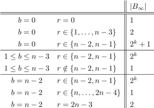
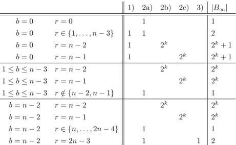
Theorem 5.1. Let 0 ≤b ≤n−2, let r∈ {b, b+ 1, . . . , b+n−1} and k∈N. The number of periodic points corresponding to

(d1, . . . , dn) = b, . . . , r−1, r+n^k, r+ 1, . . . , b+n−1 is given by Table 1.

Proof. Let (d1, . . . , dn) = b, . . . , r−1, r+n^k, r+ 1, . . . , b+n−1

, i.e.,di=b+i−1 fori6=r−b+ 1 anddi=b+i−1 +n^k fori=r−b+ 1. Letxbe an arbitrary periodic point on a cycle of length`, letσ(x) = (j₀, j₁, . . .), and leta_i=d_j_i. By Corollary 2.6,

(14)

|B_∞|

b= 0 r= 0 1

b= 0 r∈ {1, . . . , n−3} 2 b= 0 r∈ {n−2, n−1} 2^k+ 1 1≤b≤n−3 r∈ {n−2, n−1} 2^k 1≤b≤n−3 r /∈ {n−2, n−1} 1

b=n−2 r∈ {n−2, n−1} 2^k b=n−2 r∈ {n, . . . ,2n−4} 1

b=n−2 r= 2n−3 2

Table 1. The number of periodic points for some special branching function systems (see Theorem 5.1)

we havex=−y/ n^`−1

, wherey=n^`−1a_`−1+· · ·+na1+a0; moreover, {ai} is a periodic sequence whose shortest period is`.

Let us define the following two modified sequences of coefficients (here, and in the sequel, and⊕stand for subtraction and addition modulo `, respectively):

a⁰_i:=

ai−n^k, ifai=r+n^k;

ai, otherwise; a⁰⁰_i :=

a⁰_i+ 1, ifa⁰_{i k}=r;

a⁰_i, otherwise.

Note that 0≤a⁰⁰_i ≤b+n≤2n−2 for alli∈ {0, . . . , `−1}. We can now expressymod- ulon^`−1 with these new coefficients, usings≡t (mod`) =⇒ n^s≡n^t modn^`−1

:

y= X

i=0,...,`−1

a⁰_inⁱ+ X

i=0,...,`−1 ai=r+n^k

n^knⁱ≡ X

i=0,...,`−1

a⁰_inⁱ+ X

i=0,...,`−1 ai=r+n^k

n^i⊕k

= X

j=0,...,`−1

a⁰_jn^j+ X

j=0,...,`−1 a⁰_{j k}=r

n^j= X

j=0,...,`−1

a⁰⁰_jn^j=:y⁰⁰ modn^`−1 .

Since 0 ≤ a⁰⁰_i ≤ 2n−2, we have 0 ≤ y⁰⁰ ≤ (2n−2)P`−1

j=0n^j = 2 n^`−1 . On the other hand, y⁰⁰≡y≡0 modn^`−1

, therefore y⁰⁰∈

0, n^`−1,2 n^`−1 . We examine these three cases separately.

1) Ify⁰⁰ = 0, then a⁰⁰_i = 0 for alli, hence a⁰_i = 0 and a⁰_{i k} 6=r for alli. This happens if and only if b = 0, r 6= 0 and ai = 0 for all i. This gives us the periodic point x= 0 with `= 1.

2) Ify⁰⁰=n^`−1, thena⁰⁰_i =n−1 for alli. Indeed,−1≡n^`−1 =y⁰⁰≡a⁰⁰₀ (modn) and 0≤a⁰⁰₀ ≤2n−2 imply thata⁰⁰₀ =n−1. Then we have−1≡n^`−1−1 = (y⁰⁰−a⁰⁰₀)/n≡a⁰⁰₁ (modn) and 0≤a⁰⁰₁ ≤2n−2, hencea⁰⁰₁ =n−1. Continuing this way one can prove by induction on i that a⁰⁰_i =n−1 for every i. This happens if and only if for each i we have either a⁰_i = n−1, a⁰_{i k} 6= r or a⁰_i=n−2, a⁰_{i k} =r. Here we can distinguish three subcases.

2a) Ifr /∈ {n−2, n−1}, thena⁰_i=ai=n−1 for alli, therefore`= 1 and we obtain the periodic pointx=−1.

2b) Ifr=n−2, thena⁰_i∈ {n−1, n−2} anda⁰_{i k}=a⁰_i for alli. Thus {ai} is a k-periodic sequence with entries n−1 and n−2. (Recall that the shortest period of{ai}was`, hence`|k.) By Remark 2.7, we obtain 2^k different periodic points in this case.

2c) Ifr=n−1, thena⁰_i∈ {n−1, n−2}anda⁰_{i k} 6=a⁰_ifor alli, which implies a⁰_{i 2k} =a⁰_i. Thus {a_i} is a 2k-periodic sequence with entriesn−1 and n−2 such that the first half of the period uniquely determines the second half: a⁰_i⊕k= 2n−3−a⁰_i. (Here we must have`|2kand`-k.) Just like in case 2b), we get 2^k periodic points.