ZIPPER FRACTAL CURVES
BAL ´AZS B ´AR ´ANY, GERGELY KISS, AND ISTV ´AN KOLOSSV ´ARY
Abstract. We study the pointwise regularity of zipper fractal curves generated by affine mappings. Under the assumption of dominated splitting of index-1, we calculate the Hausdorff dimension of the level sets of the pointwise H¨older expo- nent for a subinterval of the spectrum. We give an equivalent characterization for the existence of regular pointwise H¨older exponent for Lebesgue almost every point. In this case, we extend the multifractal analysis to the full spectrum. In particular, we apply our results for de Rham’s curve.
1. Introduction and Statements
Let us begin by recalling the general definition of fractal curves from Hutchin- son [21] and Barnsley [3].
Definition 1.1. A system S = {f0, . . . , fN−1} of contracting mappings of Rd to itself is called a zipper with vertices Z = {z0, . . . , zN} and signature ε = (ε0, . . . , εN−1), εi∈ {0,1}, if the cross-condition
fi(z0) =zi+εi and fi(zN) =zi+1−εi
holds for every i = 0, . . . , N −1. We call the system a self-affine zipper if the functions fi are affine contractive mappings of the form
fi(x) =Aix+ti, for every i∈ {0,1, . . . , N−1}, where Ai ∈Rd×d invertible and ti∈Rd.
The fractal curve generated from S is the unique non-empty compact set Γ, for which
Γ =
N−1
[
i=0
fi(Γ).
If S is an affine zipper then we call Γ a self-affine curve.
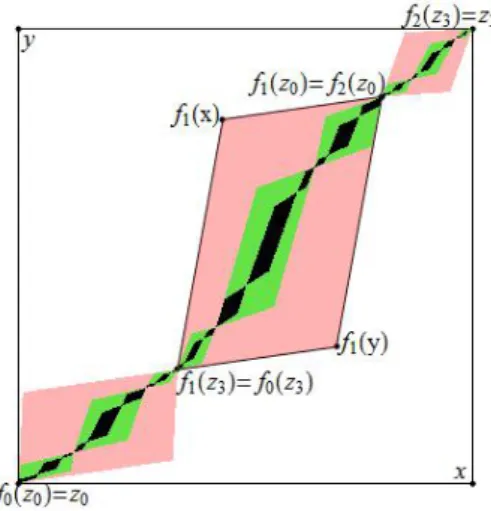
For an illustration see Figure1. It shows the first (red), second (green) and third (black) level cylinders of the image of [0,1]2. The cross-condition ensures that Γ is a continuous curve.
The dimension theory of self-affine curves is far from being well understood. The Hausdorff dimension of such curves is known only in a very few cases. The usual
Date: 10th January 2018.
2010Mathematics Subject Classification. Primary 28A80 Secondary 26A27 26A30
Key words and phrases. affine zippers, pointwise H¨older exponent, multifractal analysis, pres- sure function, iterated function system, de Rham curve.
arXiv:1608.04558v2 [math.DS] 12 Jul 2017
Figure 1. An affine zipper withN = 3 maps and signature ε= (0,1,0).
techniques, like self-affine transversality, see Falconer [14], Jordan, Pollicott and Simon [25], destroys the curve structure. Ledrappier [27] gave a sufficient condi- tion to calculate the Hausdorff dimension of some fractal curves, and Solomyak [39]
applied it to calculate the dimension of the graph of the Takagi function for typ- ical parameters. Feng and K¨aenm¨aki [17] characterized self-affine systems, which has analytic curve attractor. Let us denote the s-dimensional Hausdorff meas- ure and the Hausdorff dimension of a set A by Hs(A) and dimHA, respectively.
Moreover, let us denote the Packing and (upper) box-counting dimension of a set A by dimPA and dimBA, respectively. For basic properties and definition of Hausdorff-, Packing- and box-counting dimension, we refer to [15].
Bandt and Kravchenko [2] studied some smoothness properties of self-affine curves, especially the tangent lines of planar self-affine curves. The main pur- pose of this paper is to analyse the pointwise regularity of affine curves under some parametrization. Let us recall the definition of pointwise H¨older exponent of a real valued function g, see for example [23, eq. (1.1)]. We say that g∈Cβ(x) if there exist a δ >0,C >0 and a polynomial P with degree at most bβc such that
|g(y)−P(y−x)| ≤C|x−y|β for every y∈Bδ(x),
whereBδ(x) denotes the ball with radius δ centered atx. Letαp(x) = sup{β:g∈ Cβ(x)}. We callαp(x) thepointwise H¨older exponentof g at the point x.
We call F:Rm 7→ R a self-similar function if there exists a bounded open set U ⊂Rm, and contracting similaritiesg1, . . . , gk of Rm such thatgi(U)∩gj(U) =∅ and gi(U) ⊂ U for every i 6= j, and a smooth function g:Rm 7→ R, and real numbers |λi|<1 for i= 1, . . . , k such that
F(x) =
k
X
i=1
λiF(g−1i (x)) +g(x), (1.1) see [24, Definition 2.1]. The multifractal formalism of the pointwise H¨older expo- nent of self-similar functions was studied in several aspects, see for example Aouidi and Slimane [1], Slimane [6,7,5] and Saka [37].
Hutchinson [21] showed that the family of contracting functionsg1, . . . , gk has a unique, non-empty compact invariant set Ω (called theattractor ofΦ ={g1, . . . , gk}),
i.e. Ω =Sk
i=1gi(Ω). We note that in the case of self-similar function, the graph of F (denoted by Graph(F)) over the set Ω can be written as the unique, non-empty, compact invariant set of the family of functions S1, . . . , Sk inRm+1, where
Si(x, y) = (gi(x), λiy+g(gi(x))).
In this paper, we study the local regularity of a generalized version of self- similar functions. Namely, let λ = (λ0, . . . , λN−1) be a probability vector. Let us subdivide the interval [0,1] according to the probability vectorλand signature ε = (ε0, . . . , εN−1), εi ∈ {0,1} of the zipper S. Let gi be the linear function mapping the unit interval [0,1] to theith subinterval of the division which is order- preserving or order-reversing according to the signature εi. That is, the interval [0,1] is the attractor of the iterated function system
Φ ={gi:x7→(−1)εiλix+γi}N−1i=0 , (1.2) where γi = Pi−1
j=0λj +εiλi. Let v : [0,1] 7→ Γ ⊂ Rd be the unique continuous function satisfying the functional equation
v(x) =fi v(g−1i (x))
ifx∈gi([0,1]). (1.3) We note that gi−1(x) = (−1)x−γεiiλ
i, and g−1i (x) ∈ [0,1] if and only if x ∈ gi([0,1]).
Thus, Graph(v) is the attractor of the IFS
Si(x, y) = (gi(x), Aiy+ti).
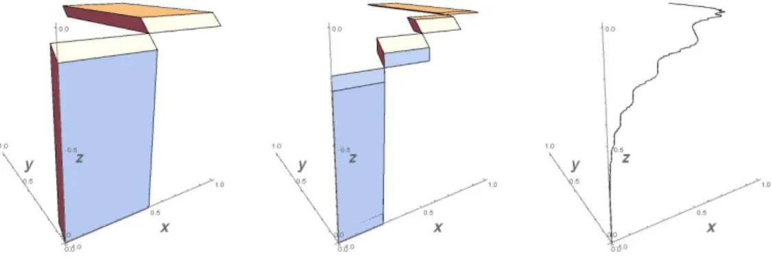
We call v as the linear parametrization of Γ. Such linear parameterizations occur in the study of Wavelet functions in a natural way, see for example Protasov [35], Protasov and Guglielmi [36], and Seuret [38]. A particular example for (1.3) is the de Rham’s curve, see Section 5 for details including an example of a graph of v generated by the de Rham’s curve.
The main difference between the self-similar function F defined in (1.1) and v defined in (1.3) is the contraction part. Namely, whileF is a real valued function rescaled by only a real number, the function v is Rd valued and a strict affine transformation is acting on it. This makes the study of such functions more difficult.
As a slight abuse of the appellation of the pointwise H¨older exponent, we redefine the pointwise H¨older exponent α(x) of the function v at a pointx∈[0,1] as
α(x) = lim inf
y→x
logkv(x)−v(y)k
log|x−y| . (1.4)
We note that ifαp(x)<1 orα(x)<1 thenαp(x) =α(x). Otherwise, we have only α(x)≤αp(x).
When the lim inf in (1.4) exists as a limit, then we say that v has a regular pointwise H¨older exponent αr(x) at a pointx∈[0,1], i.e.
αr(x) = lim
y→x
logkv(x)−v(y)k
log|x−y| . (1.5)
Let us define the level sets of the (regular) pointwise H¨older exponent by E(β) ={x∈[0,1] :α(x) =β} and
Er(β) ={x∈[0,1] :αr(x) =β}.
Our goal is to perform multifractal analysis, i.e. to study the possible values, which occur as (regular) pointwise H¨older exponents, and determine the magnitude
of the sets, where it appears. This property was studied for several types of sin- gular functions, for example for wavelets by Barral and Seuret [4], Seuret [38], for Weierstrass-type functions Otani [32], for complex analogues of the Takagi function by Jaerisch and Sumi [22] or for different functional equations by Coiffard, Melot and Willer [10], by Okamura [31] and by Slimane [7] etc.
The main difficulty in our approach is to handle the distance kv(x)−v(y)k. In the previous examples, the function F defined with the equation (1.1) was scaled only by a constant. Roughly speaking
kF(gi1,...,in(x))−F(gi1,...,in(y))k ≈ |λi1· · ·λin|kF(x)−F(y)k.
In the case of self-affine systems, this is not true anymore. That is, kv(gi1,...,in(x))−v(gi1,...,in(y))k ≈ kAi1· · ·Ain(v(x)−v(y))k.
However, in general kAi1· · ·Ain(v(x)−v(y))k 6≈ kAi1· · ·Ainkkv(x)−v(y)k. In order to be able to compare the distance kv(gi1,...,in(x))−v(gi1,...,in(y))k with the norm of the product of matrices, we need an extra assumption on the family of matrices.
Let us denote by Mo the interior and by M the closure of a set M ⊆ PRd−1. For a pointv∈Rd, denotehviequivalence class ofvin the projective spacePRd−1. Every invertible matrixA defines a natural map on the projective spacePRd−1 by hvi 7→ hAvi. As a slight abuse of notation, we denote this function byA too.
Definition 1.2. We say that a family of matricesA={A0, . . . , AN−1} have dom- inated splitting of index-1 if there exists a non-empty open subsetM ⊂PRd−1 with a finite number of connected components with pairwise disjoint closure such that
N−1
[
i=0
AiM ⊂Mo,
and there is a d−1 dimensional hyperplane that is transverse to all elements of M. We call the set M a multicone.
We adapted the definition of dominated splitting of index-1 from the paper of Bochi and Gourmelon [8]. They showed that the tuple of matrices A satisfies the property in Definition 1.2if and only if there exist constantsC >0 and 0< τ <1 such that
α2(Ai1· · ·Ain)
α1(Ai1· · ·Ain) ≤Cτn
for every n ≥ 1 and i0, . . . , in−1 ∈ {0, . . . , N −1}, where αi(A) denotes the ith largest singular value of the matrix A. That is, the weakest contracting direction and the stronger contracting directions are strongly separated away (splitted), α1 dominatesα2. This condition makes it easier to handle the growth rate of the norm of matrix products, which will be essential in our later studies.
We note that for example a tuple A formed by matrices with strictly positive elements, satisfies the dominated splitting of index-1 of M =h{x∈Rd:xi >0, i= 1, . . . , d}i. Throughout the paper we work with affine zippers, where we assume that the matrices Ai have dominated splitting of index-1. For more details, see Section 2and [8].
For a subset M ofPRd−1 and a pointx∈Rd, let M(x) ={y∈Rd:hy−xi ∈M}.
We call the set M(x) a cone centered at x.
We say that S satisfies the strong open set condition (SOSC), if there exists an open bounded set U such that
fi(U)∩fj(U) =∅ for everyi6=j and Γ∩U 6=∅.
We call S a non-degenerate system, if it satisfies the SOSC and hzN − z0i ∈/ T∞
k=0
T
|ı|=kA−1ı (Mc), where for a finite length word ı = i1. . . ik, Aı denotes the matrix productAi1Ai2. . . Aik. We note that the non-degenerate condition guaran- tees that the curve v: [0,1]7→Rd is not self-intersecting and it is not contained in a strict hyperplane of Rd.
Denote by P(t) the pressure function which is defined as the unique root of the equation
0 = lim
n→∞
1 nlog
N−1
X
i1,...,in=0
kAi1· · ·Ainkt(λi1· · ·λin)−P(t). (1.6) A considerable attention has been paid for pressures, which are defined by mat- rix norms, see for example K¨aenm¨aki [26], Feng and Shmerkin [19], and Morris [28, 29]. Feng [16] and later Feng and Lau [18] studied the properties of the pres- sureP for positive and non-negative matrices. In Section2, we extend these results for the dominated splitting of index-1 case. Namely, we will show that the func- tion P : R 7→ R is continuous, concave, monotone increasing, and continuously differentiable.
Unfortunately, even for positive matrices, the computation of the precise values of P(t) is hopeless. For a fast approximation algorithm, see Pollicott and Vyt- nova [33].
Let d0 >0 be the unique real number such that 0 = lim
n→∞
1
nlog X
|ı|=n
kAıkd0. (1.7)
Observe that for every n≥1,{fı(U) :|ı|=n}defines a cover of Γ. But since Γ is a curve and thus dimHΓ≥1, and since everyfı(U) can be covered by a ball with radius kAık|U|,d0≥1.
Let
αmin= lim
t→+∞
P(t)
t , αmax= lim
t→−∞
P(t)
t and αb=P0(0).
The values αmin and αmax correspond to the logarithm of the joint- and the lower-spectral radius defined by Protasov [35].
We say that the function v: [0,1]7→Γ issymmetric if λ0 =λN−1 and lim
k→∞
kAk0k
kAkN−1k = 1. (1.8)
Now, we state our main theorems on the pointwise H¨older exponents.
Theorem 1.3. Let S be a non-degenerate system. Then there exists a constant αb such that for L-a.e. x ∈[0,1], α(x) = αb ≥1/d0. Moreover, there exists an ε >0 such that for every β∈[α,b αb+ε]
dimH{x∈[0,1] :α(x) =β}= inf
t∈R
{tβ−P(t)}. (1.9) If S satisfies (1.8) then (1.9) can be extended for every β ∈[αmin,αb+ε].
Furthermore, the functionsβ 7→dimHE(β)andβ 7→dimHEr(β)are continuous and concave on their respective domains.
In the following, we give a sufficient condition to extend the previous result, where (1.9) holds to the complete spectrum [αmin, αmax]. As a slight abuse of notation for every θ∈PRd−1, we say that 06=v ∈θ ifhvi=θ.
Assumption A. For a nondegenerate affine zipper S = {fi:x7→Aix+ti}N−1i=0 with vertices{z0, . . . , zN}assume that there exists a convex, simply connected closed cone C ⊂PRd−1 such that
(1) SN
i=1AiC⊂Co and for every 06=v ∈θ∈C, hAiv, vi>0, (2) hzN −z0i ∈Co.
Observe that if S satisfies Assumption A then it satisfies the strong open set condition with respect to the set U, which is the bounded component of Co(z0)∩ Co(zN). We note that if all the matrices have strictly positive elements and the zipper has signature (0, . . . ,0) then Assumption A holds.
Theorem 1.4. Let S be an affine zipper satisfying Assumption A. Then for every β ∈[α, αb max]
dimH{x∈[0,1] :α(x) =β}= inf
t∈R
{tβ−P(t)}, (1.10) and for every β∈[αmin, αmax]
dimH{x∈[0,1] :αr(x) =β}= inf
t∈R
{tβ−P(t)}. (1.11) Moreover, ifS satisfies(1.8)then (1.10)can be extended for everyβ ∈[αmin, αmax].
The functionsβ7→dimHE(β)andβ 7→dimHEr(β)are continuous and concave on their respective domains.
Assumption A has another important role. In Theorem 1.4, we calculated the spectrum for the regular H¨older exponent, providing that it exists. We show that the existence of the regular H¨older exponent for Lebesgue typical points is equival- ent to Assumption A.
Theorem 1.5. Let S be a non degenerate system. Then the regular H¨older expo- nent exists for Lebesgue almost every point if and only if S satisfies Assumption A. In particular, αr(x) =P0(0) for Lebesgue almost every x∈[0,1].
Remark 1.6. In the sequel, to keep the notation tractable we assume the signature ε= (0, . . . ,0). The results carry over for general signatures, and the proofs can be easily modified for the general signature case, see Remark 5.3.
The organization of the paper is as follows. In Section2we prove several proper- ties of the pressure functionP(t), extending the works of [16,18] to the dominated splitting of index-1 case using [8]. We prove Theorem 1.3 in Section 3. Section 4 contains the proofs of Theorems1.4 and 1.5when the zipper satisfies Assumption A. Finally, as an application in Section 5, we show that our results can be applied to de Rham’s curve, giving finer results than existing ones in the literature.
2. Pressure for matrices with dominated splitting of index-1 In this section, we generalize the result of Feng [16], and Feng and Lau [18].
In [18] the authors studied the pressure function and multifractal properties of
Lyapunov exponents for products of positive matrices. Here, we extend their results for a more general class of matrices by using Bochi and Gourmelon [8] for later usage.
Let Σ be the set of one side infinite length words of symbols {0, . . . , N−1}, i.e.
Σ = {0, . . . , N −1}N. Let σ denote the left shift on Σ, its n-fold composition by σni= (in+1, in+2, . . .). We use the standard notationi|nfori1, . . . , in and
[i|n] :={j∈Σ :j1 =i1, . . . , jn=in}. Let us denote the set of finite length words by Σ∗ =S∞
n=0{0, . . . , N−1}n, and for an ı∈Σ∗, let us denote the length of ı by |ı|. For a finite wordı∈Σ∗ and for a j∈Σ, denoteıjthe concatenation of the finite word ıwith j.
Denote i∧j the length of the longest common prefix of i,j ∈ Σ, i.e. i∧j = min{n−1 : in6=jn}. Letλ= (λ0, . . . , λN−1) be a probability vector and letd(i,j) be the distance on Σ with respect to λ. Namely,
d(i,j) =
i∧j
Y
n=1
λin =:λi|i∧j.
If i∧j= 0 then by definition i|i∧j =∅ and λ∅ = 1. For every r > 0, we define a partition Ξr of Σ by
Ξr =
[i1, . . . , in] :λi1· · ·λin ≤r < λi1· · ·λin−1 . (2.1) For a matrixAand a subspaceθ, denotekA|θkthe norm ofArestricted toθ, i.e.
kA|θk= supv∈θkAvk/kvk. In particular, ifθhas dimension onekA|θk=kAvk/kvk for any 0 6= v ∈ θ. Denote G(d, k) the Grassmanian manifold of k dimensional subspaces of Rd. We define the angle between a 1 dimensional subspace E and a d−1 dimensional subspaceF as usual, i.e.
^(E, F) = arccos
hv,projFvi kprojFvkkvk
,
where 0 6=v∈E arbitrary and projF denotes the orthogonal projection onto F.
The following theorem collects the most relevant properties of a family of matrices with dominated splitting of index-1.
Theorem 2.1. [8, Theorem A, Theorem B, Claim on p. 228]Suppose that a finite set of matrices {A0, . . . , AN−1} satisfies the dominated splitting of index-1 with multicone M. Then there exist H¨older continuous functions E : Σ 7→ PRd−1 and F : Σ7→G(d, d−1)such that
(1) E(i) =Ai1E(σi) for every i∈Σ, (2) F(i) =A−1i
1 F(σi) for every i∈Σ,
(3) there exists β >0 such that^(E(i), F(j))> β for everyi,j∈Σ, (4) there exist constants C≥1 and 0< τ <1 such that
α2(Ai|n)
kAi|nk ≤Cτn for everyi∈Σand n≥1,
(5) there exists a constant C >0 such that kAi|n|E(σni)k ≥CkAi|nk for every i∈Σ,
(6) there exists a constantC >0 such thatkAi|n|F(in. . . i1j)k ≤Cα2(Ai|n) for every i,j∈Σ.
In particular, if M is the multicone from Definition 1.2, then E(i) =
∞
\
n=1
Ai1· · ·Ain(M),
and for everyV ∈M,Ai1· · ·AinV →E(i) uniformly (independently ofV). Hence, there exists a constant C >0 such that for everyV ∈M and everyı∈Σ∗,
kAı|Vk ≥C0kAık. (2.2)
So, this gives us a strong control over the growth rate of matrix products on subspaces in M.
Another consequence of Theorem2.1is that the functionψ(i) = logkAi1|E(σi)k is H¨older-continuous. That is, there exist C >0 and 0< τ <1 such that
|ψ(i)−ψ(j)| ≤Cτi∧j. (2.3) Moreover, by the property E(i) =Ai1E(σi), we have
kAi|n|E(σni)k=
n
Y
k=1
kAik|E(σki)k. (2.4)
Indeed, since E(i) is a one dimensional subspace, for everyv∈E(σni) kAi|n|E(σni)k= kAi|nvk
kvk =
n
Y
k=1
kAik...invk kAik+1,...,invk =
n
Y
k=1
kAik|E(σki)k.
Remark 2.2. We note if the multicone M in Definition 1.2 has only one connec- ted component then it can be chosen to be simply connected and convex. Indeed, since M is separated away from the strong stable subspacesF thencv(M) must be separated away from every d−1dimensional strong stable subspace, as well, where cv(M) denotes the convex hull of M. Thus Ai(cv(M))⊂cv(M)o for every i.
For every t, let ϕt: Σ7→R be the potential function defined by ϕt(i) = log
kAi1|E(σi)ktλ−P(t)i1
, (2.5)
where P(t) was defined in (1.6).
Using Theorem 2.1, one can show that for every t, ϕt is a H¨older continuous function. Thus, by [9, Theorem 1.4], for every t ∈ R there exists a unique σ- invariant, ergodic probability measure µt on Σ such that there exists a constant C(t)>1 such that for everyi∈Σ and every n≥1
C(t)−1≤ µt([i|n]) Qn−1
k=0eϕt(σki) ≤C(t). (2.6) Observe that
n−1
Y
k=0
eϕt(σki) =kAi|n|E(σni)kt·λ−Pi| (t)
n .
Moreover,
dimHµt= hµt
χµt
, (2.7)
where
hµt = lim
n→∞
−1 n
X
|ı|=n
µt([ı]) logµt([ı]) =− Z
ϕt(i)dµt(i), (2.8) χµt = lim
n→∞
−1 n
X
|ı|=n
µt([ı]) logλı =− Z
logλi1dµt(i). (2.9) We call χµt the Lyapunov exponent of µt and hµt the entropy of µt.
Lemma 2.3. The map t7→P(t) is continuous, concave, monotone increasing on R.
Proof. Since µtis a probability measure on Σ and Ξr is a partition we get 0 = logP
ı∈Ξrµt([ı])
logr for every r >0 and by (2.6) and (1.6)
P(t) = lim
r→0+
logP
ı∈ΞrkAıkt
logr . (2.10)
Using this form it can be easily seen that t 7→ P(t) is continuous, concave and
monotone increasing.
By Lemma2.3, the potentialϕtdepends continuously on t. Moreover, by (2.3),
|ϕ(i)−ϕ(j)| ≤Ctτi∧j. Thus, the Perron-Frobenius operator (Tt(g))(i) =
N−1
X
i=0
eϕt(ii)g(ii)
depends continuously on t. Hence, the unique eigenfunction htofTtand the eigen- measure ofνtof the dual operatorTt∗ depends continuously ont. Sincedµt=htdνt, see [9, Theorem 1.16], we got thatt7→µt is continuous in weak*-topology. Hence, by (2.8) and (2.9),t7→hµt andt7→χµt are continuous onR.
Proposition 2.4. The mapt7→P(t)is continuously differentiable onR. Moreover, for every t∈R
dimHµt=tP0(t)−P(t), and
n→∞lim
logkAi1· · ·Aink logλi1· · ·λin
=P0(t) for µt-almost everyi∈Σ.
Proof. We recall [20, Theorem 2.1]. That is, sinceµt is a Gibbs measure τµt(q) = lim
r→0+
logP
ı∈Ξrµt([ı])q logr
is differentiable at q = 1 and τµ0t(1) = dimHµt. On the other hand, by (2.6) and (2.10)
τµt(q) =P(tq)−P(t)q.
Hence, by taking the derivative atq= 1 we get thatP(t) is differentiable for every t∈R/{0} and
dimHµt=tP0(t)−P(t).
Let us observe that by (2.5), (2.7) and (2.8) dimHµt=t−R
logkAi1|E(σi)kdµt(i)
−R
logλi1dµt(i) −P(t).
Thus,
P0(t) = −R
logkAi1|E(σi)kdµt(i)
−R
logλi1dµt(i) for everyt6= 0.
Since t7→µt is continuous in weak*-topology we get that t7→ P0(t) is continuous on R/{0}. On the other hand, the left and right hand side limits of P0(t) att= 0 exist and are equal. Thus, t7→P(t) is continuously differentiable on R.
By Theorem2.1and ergodicity of µtwe get the last assertion of the proposition.
Let us observe that by the definition of pressure function (1.6),P(0) =−1 and thus,µ0corresponds to the Bernoulli measure on Σ with probabilities (λ0, . . . , λN−1).
That is,
µ0([i1, . . . , in]) =λi1· · ·λin.
Lemma 2.5. For every finite set of matricesAwith dominated splitting of index-1, P0(0)≥1/d0, P0(d0)≤1/d0. Moreover, P0(0)>1/d0 if and only if P0(d0)<1/d0
if and only if µd0 6=µ0.
Proof. By the definition of P(t), (1.6), P(d0) = 0, where d0 is defined in (1.7).
Together withP(0) =−1 and the concavity and differentiability ofP(t) (by Lemma 2.3 and Proposition 2.4), we get P0(0)≥1/d0,P0(d0) ≤1/d0. Moreover,P0(0) >
1/d0 if and only if P0(d0)<1/d0.
On the other hand, by Proposition 2.4 dimHµd0 =d0P0(d0) = lim
n→∞
logkAi|nkd0
logλi|n = hµd
0
χµd0
forµd0-a.e. i,
where in the last equation we used the definition of µd0, the entropy and the Lyapunov exponent. Since dimHµ0 = 1, if P0(d0) <1/d0 then µ0 6=µd0. On the other hand, by [9, Theorem 1.22], for everyσ-invariant, ergodic measureν on Σ,
hν
−R
logλi0dν(i) ≤1 and hν
−R
logλi0dν(i) = 1 if and only if ν =µ0. Therefore, if P0(d0) = 1/d0 then hχµd0
µd0
= 1 and so µd0 =µ0.
Lemma 2.6. For every α∈[αmin, αmax] dimH
n
i∈Σ : lim inf
m→∞
logkAi|mk logλi|m ≤α
o
≤inf
t≥0{tα−P(t)} (2.11) and
dimHn
i∈Σ : lim sup
m→∞
logkAi|mk logλi|m
≥αo
≤inf
t≤0{tα−P(t)} (2.12) Proof. For simplicity, we use the notations
Gα =
i∈Σ : lim inf
m→∞
logkAi|mk logλi|m ≤α
and Gα=
i∈Σ : lim sup
m→∞
logkAi|mk logλi|m ≥α
.
Letε >0 be arbitrary but fixed and let us define the following sets of cylinders:
Dr(ε) = n
[ı]∈Ξρ: 0< ρ≤r and logkAık logλı
≤α+ε o
and
Dr(ε) =n
[ı]∈Ξρ: 0< ρ≤r and logkAık logλı
≥α−εo .
By definition,Dr(ε) is a cover ofGα and respectively,Dr(ε) is a cover ofGα. Now let Cr(ε) andCr(ε) be a disjoint set of cylinders such that
[
[ı]∈Dr(ε)
[ı] = [
[ı]∈Cr(ε)
[ı] and [
[ı]∈Dr(ε)
[ı] = [
[ı]∈Cr(ε)
[ı].
Then by (2.6) and the definition of Cr(ε), for any t≥0 Hαt−P(t)+(1+t)ε
r (Gα)≤ X
[ı]∈Cr(ε)
λ(αt−P(t)+(1+t)ε) ı
≤λ−1minrε X
[ı]∈Cr(ε)
kAıktλ−Pı (t)
≤Cλ−1minrε X
[ı]∈Cr(ε)
µt([ı])≤Cλ−1minrε.
Hence,Hαt−P(t)+(1+t)ε(Gα) = 0 for anyt >0 and anyε >0, so (2.11) follows. The proof of (2.12) is similar by using the coverCr(ε) of Gα.
We note that by the concavity of P
t∈infR
{tα−P(t)}= inf
t≤0{tα−P(t)}, for every and α∈[P0(0), αmax],
t∈infR
{tα−P(t)}= inf
t≥0{tα−P(t)}, for every α∈[αmin, P0(0)].
3. Pointwise H¨older exponent for non-degenerate curves First, let us define the natural projections π and Π from the symbolic space Σ to the unit interval [0,1] and the curve Γ. We recall that we assumed that all the signatures of the affine zipper Definition1.1is 0, and all the matrices are invertible.
Therefore,
π(i) = lim
n→∞gi1◦ · · · ◦gin(0) =
∞
X
n=1
λi|n−1γin (3.1) Π(i) = lim
n→∞fi1 ◦ · · · ◦fin(0) =
∞
X
n=1
Ai|n−1tin. (3.2) Observe that by the definition of the linear parametrization vof Γ, v(π(i)) = Π(i).
In the analysis of the pointwise H¨older exponent α, defined in (1.4), the points play important role which are far away symbolically but close on the self-affine curve. To be able to handle such points we introduce the following notation
i∨j=
min{σi∧j+1i∧N−1, σi∧j+1j∧0}, ifii∧j+1+ 1 =ji∧j+1, min{σi∧j+1i∧0, σi∧j+1j∧N−1}, ifji∧j+1+ 1 =ii∧j+1,
0, otherwise,
where 0denotes the (0,0, . . .) and N−1denotes the (N−1, N−1, . . .) sequence.
It is easy to see that there exists a constant K >0 such that
K−1(λi|i∧j+i∨j+λj|i∧j+i∨j)≤ |π(i)−π(j)| ≤K(λi|i∧j+i∨j+λj|i∧j+i∨j). (3.3) Hence, the distance on [0,1] is not comparable with the distance on the symbolic space. More precisely, let T be the set of points on the symbolic space, which has tail 0 or N −1, i.e. i ∈ T if and only if there exists a k ≥ 0 such that σki = 0 or σki = N−1. So if π(σki) is too close to the set π(T) infinitely often then we lose the symbolic control over the distance |π(i)−π(in)|, where in is such that π(in)→π(i) as n→ ∞.
On the other hand, the symbolic control of the setkΠ(i)−Π(in)kis also far non- trivial. In general,kΠ(i)−Π(j)k=kAi|i∧j(Π(σi∧ji)−Π(σi∧jj))kis not comparable to kAi|i∧jk · kΠ(σi∧ji)−Π(σi∧jj)k, unless hΠ(σi∧ji)−Π(σi∧jj)i ∈ M, where M is the multicone satisfying the Definition 1.2. Thus, in order to handle
lim inf
n→∞
logkΠ(i)−Π(in)k log|π(i)−π(in)|
we need that i is sufficiently far from the tail set T and also that the points Π(in) on Γ can be chosen such that hΠ(σi∧ji)−Π(σi∧inin)i ∈M. So we introduce a kind of exceptional set B, where both of these requirements fail. We defineB ⊆Σ such that
B =
i∈Σ :∀0 n≥1 ∀0 l≥1 ∀0 m≥1 ∃0 K ≥0 ∀0 k≥K
M(Π(σki))\B1/n(Π(σki))
∩Γ\(Γσki|l∪Γσki|l−1(ik+l−1)(N−1)m∪Γσki|l−1(ik+l+1)0m) =∅o , (3.4) where Γı=fı(Γ) for any finite length wordı∈Σ∗andM(Π(i)) is the cone centered
at Π(i). We note that ifil = 0 (oril=N−1) then we define Γσki|l−1(il−1)(N−1)m =∅ (or Γσki|l−1(il+1)0m =∅ respectively).
In particular, B contains those pointsi, for which locally the curve Γ will leave the cone M very rapidly. In other words, let
Bn,l,m={i∈Σ :
M(Π(i))\B1/n(Π(i))
∩Γ\(Γi|l∪Γi|l−1(il−1)(N−1)m∪Γi|l−1(il+1)0m) =∅ . and
Bn,m,l,K =
∞
\
k=K
σ−kBn,l,m and B =
∞
\
n=1
∞
\
l=0
∞
\
m=0
∞
[
K=0
Bn,l,m,K.
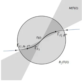
For a visualisation of the local neighbourhood of a point inBn,l,m, see Figure 2.
In particular, we are able to handle the pointwise H¨older exponents atπ(i) outside to the set B and we show that B is small in some sense.
Figure 2. Local neighbourhood of points inBn,l,m.
Lemma 3.1. Let us assume that S is non-degenerate. Then there exist n ≥ 1, l≥1, m≥1 and finite length word with||=l, such that
Bn,l,m∩[] =∅.
Proof. Our first claim is that there exists a finite sequence ı such that hAı(zN − z0)i ∈M. Suppose that this is not the case. That is, for every finite length word hAı(zN −z0)i ∈ Mc. Equivalently, for every finite length word ı, hzN −z0i ∈ A−1ı (Mc). Thus, hzN −z0i ∈T∞
k=0
T
|ı|=kA−1ı (Mc), which contradicts to our non- degeneracy assumption.
Let us fix an ı such that hAı(zN −z0)i ∈ M. Then fı(zN) ∈ M(fı(z0)). By continuity, one can choose k≥1 large enough such that for everyi∈[ı0k],
fı(zN)∈M(Π(i)) and
kfı(z0)−Π(i)k=kAı0k(z0−Π(σ|ı|+ki))k ≤ kAıkkAk0kdiam(Γ)≤ 1
2kAı(zN−z0)k, . where we used the fact that f0(z0) =z0. Then
kΠ(i)−fı(zN)k ≥ kAı(zN −z0)k − kfı(z0)−Π(i)k> 1
2kAı(zN −z0)k.
We get that for every i∈[ı0k] fı(zN)∈
M(Π(i))\B1
2kAı(zN−z0)k(Π(i))
∩Γ\(Γı0k∪Γı0k−110∪Γı|
|ı|−1(ı|ı|−1)N)6=∅.
By fixing:=ı0k,l:=||,m:= 1 andn:=l
2 kAı(zN−z0)k
m
, we see thatBn,l,m∩[] =
∅.
Proposition 3.2. Let us assume that S is non-degenerate. Then dimPπ(B)<1.
Moreover, for any ν fully supported ergodic measure on Σ, ν(B) = 0.
Proof. By definition, Bn,l,m ⊇Bn+1,l,m, Bn,l,m ⊇Bn,l+1,m and Bn,l,m ⊇Bn,l,m+1. Moreover, Bn,l,m,K =σ−KBn,l,m,0. In particular,σ−1Bn,l,m,0 =Bn,l,m,1⊇Bn,l,m,0. Thus, for every n≥1
Bn,l,m,0⊆ [
|ı|=q
%ı(Bn,l,m,0), (3.5)
where%ı(i) =ıi. Letn0 ≥1,l0≥1,m0 ≥1 be natural numbers and be the finite length word with ||=l0 as in Lemma3.1, then
Bn0,l0,m0,0∩[] =
∞
\
k=0
σ−kBn0,m0,l0 ∩[]
⊆Bn0,m0,l0 ∩[] =∅.
Thus,
Bn0,l0,m0,0⊆ [
|ı|=l0
ı6=
%ı(Bn0,l0,m0,0). (3.6) Hence, σpi∈/[] for every i∈Bn0,l0,m0,0 and for every p≥1. Indeed, if there exist i ∈Bn0,l0,m0,0 and p≥1 such that σpi∈[] then there exist a finite length wordı with |ı|=p such thatB∩[ı]6=∅. But by equations (3.5) and (3.6),
Bn0,l0,m0,0 ⊆ [
|ı1|=p
%ı1(Bn0,l0,m0,0)⊆ [
|ı1|=p
[
|ı2|=l0
ı26=
%ı1(%ı2(Bn0,l0,m0,0))⊆ [
|ı1|=p
[
|ı2|=l0
ı26=
[ı1ı2]
which is a contradiction. But for any fully supported ergodic measureν,ν([])>0 and therefore ν(Bn0,l0,m0,0) = 0. The second statement of the lemma follows by
ν(B)≤ inf
n,l,mν(
∞
[
K=0
Bn,l,m,K)≤
∞
X
K=0
ν(Bn0,l0,m0,K) =
∞
X
K=0
ν(Bn0,l0,m0,0) = 0.
To prove the first assertion of the proposition, observe that by equation (3.6) π(Bn0,l0,m0,0)⊆ [
|ı|=l0
ı6=
gı(π(Bn0,l0,m0,0)).
Therefore, π(Bn0,l0,m0,0) is contained in the attractor Λ of the IFS {gı}|ı|=l0
ı6=
, for which dimBΛ<1. Hence,
dimP π(B)≤ inf
n,l,mdimBπ(Bn,l,m,0)≤dimBπ(Bn0,l0,m0,0)≤dimBΛ<1.
Lemma 3.3. Let us assume that S is non-degenerate. Then for every i∈Σ\B
α(π(i))≤lim sup
n→+∞
logkAi|nk logλi|n
.
Proof. Leti∈Σ\B. Then there exist n≥1,l≥1,m≥1 and a sequence{kp}∞p=1 such that kp → ∞ asp→ ∞and
M(Π(σkpi))\B1/n(Π(σkpi))
∩
Γ\(Γσkpi|l∪Γσkpi|l−1(ikp+l−1)(N−1)m∪Γσkpi|l−1(ikp+l+1)0m)6=∅ (3.7)
Hence, there exists a sequence jp such that kp ≤i∧jp ≤kp+l,i∨jp ≤m, Π(σkpjp)∈M(Π(σkpi)) andkΠ(σkpjp)−Π(σkpi)k> 1
n. (3.8)
Thus,
α(π(i)) = lim inf
π(j)→π(i)
logkΠ(i)−Π(j)k
log|π(i)−π(j)| ≤lim inf
p→+∞
logkΠ(i)−Π(jp)k log|π(i)−π(jp)| = lim inf
p→+∞
logkAi|kp(Π(σkpi)−Π(σkpjp))k
log|λi|i∧jp+i∨jp(π(σi∧jp+i∨jpi)−π(σi∧jp+i∨jpjp))|, and by (2.2), (3.8),
lim inf
p→+∞
logkAi|kp(Π(σkpi)−Π(σkpjp))k
log|λi|i∧jp+i∨jp(π(σi∧jp+i∨jpi)−π(σi∧jp+i∨jpjp))|≤ lim inf
p→+∞
log(C−1/n) + logkAi|
kpk
logλi|kp+ logd0 ≤lim sup
p→+∞
logkAi|pk logλi|p ,
where d0 = (maxiλi)m+l.
Lemma 3.4. Let us assume that S is non-degenerate. Then for every ergodic,σ- invariant, fully supported measure µonΣsuch thatP∞
k=0(µ[0k] +µ([Nk])is finite, then
α(π(i)) = lim
n→+∞
logkAi|nk
logλi|n for µ-a.e. i∈Σ.
Proof. By Proposition3.2, we have thatµ(B) = 0. Thus, by Lemma3.3, forµ-a.e.
i
α(π(i))≤ lim
n→+∞
logkAi|nk logλi|n . On the other hand, for everyi∈Σ,
α(π(i)) = lim inf
π(j)→π(i)
logkΠ(i)−Π(j)k
log|π(i)−π(j)| ≥lim inf
j→i
logkAi|i∧jk
logλi|i∧j+i∨j+ log miniλi. Hence, to verify the statement of the lemma, it is enough to show that
limj→i
logλi|i∧j logλi|i∧j+i∨j
= 1 forµ-a.e. i.
It is easy to see that from limj→ii∨j
i∧j = 0 follows the previous equation. Let Rn=
i:∃jk s. t. jk→i ask→ ∞ and lim
k→∞
i∨jk i∧jk > 1
n
In other words, Rn=
∞
\
K=0
∞
[
k=K N
[
i1,...,ik=0
[i1, . . . , ik,
bk/nc
z }| {
0, . . . ,0]∪[i1, . . . , ik,
bk/nc
z }| { N, . . . , N]
Therefore, for any µergodic σ-invariant measure and for everyK ≥0 µ(Rn)≤
∞
X
k=K
(µ([0bk/nc]) +µ([Nbk/nc])).
Since by assumption the sum on the right hand side is summable, we getµ(Rn) = 0
for every n≥1.
Let us recall that we call the function v: [0,1]7→Γsymmetric if λ0 =λN−1 and lim
k→∞
kAk0k
kAkN−1k = 1. (3.9)
Lemma 3.5. Let us assume that S is non-degenerate and symmetric. Then for every i∈Σ
α(π(i))≥lim inf
n→+∞
logkAi|nk logλi|n
.
Proof. Let us observe that by the zipper propertyfi(Π(0)) =fi−1(N−1) for every 1≤i≤N−1. Moreover, for anyi,jwithii∧j+1=ji∧j+1+ 1,
i∨j= min{σi∧j+1i∧N−1, σi∧j+1j∧0}.
Thus, ifii∧j+1 =ji∧j+1+ 1
kΠ(i)−Π(j)k=kΠ(i)−Π(i|i∧jii∧j+10) + Π(j|i∧jji∧j+1N−1)−Π(j)k
=kAi|i∧j+i∨j(Π(σi∧j+i∨ji)−Π(0)) +Ai|i∧j+i∨j(Π(N−1)−Π(σi∧j+i∨jj))k
≤(kAi|i∧j+i∨jk+kAj|i∧j+i∨jk)diam(Γ). (3.10)
The case ii∧j+1 = ji∧j+1−1 is similar, and if |ii∧j+1−ji∧j+1| 6= 1 then i∨j= 0, so (3.10) holds trivially. Moreover by (3.3), there exist constants K1, K2 >0 such that for every i,j∈Σ
logkΠ(i)−Π(j)k
log|π(i)−π(j)| ≥ −logK1+ log(kAi|i∧j+i∨jk+kAj|i∧j+i∨jk)
log(λi|i∧j+i∨j+λj|i∧j+i∨j) + logK2 . (3.11) Therefore,
α(π(i)) = lim inf
π(j)→π(i)
logkΠ(i)−Π(j)k log|π(i)−π(j)| ≥ lim inf
j→i
−logK1+ log(kAi|i∧j+i∨jk+kAj|i∧j+i∨jk) log(λi|i∧j+i∨j+λj|i∧j+i∨j) + logK2
=
lim inf
j→i
logkAi|i∧j+i∨jk
−logkAlogK1
i|i∧j+i∨jk + 1 +
log 1+
kAj|i∧j+i∨jk kAi|i∧j+i∨jk
!
logkAi|i∧j+i∨jk
logλi|i∧j+i∨j
1 +loglog 2Kλ 2
i|i∧j+i∨j
.
So, to verify the statement of the lemma, it is enough to show that there exists a constantC >0 such that for every, i,j∈Σ
C−1≤ kAj|i∧j+i∨jk kAi|i∧j+i∨jk ≤C.
By Theorem 2.1(5) and (2.4), there existC0 >0 such that
kAi|i∧j+i∨jk ≥ kAi|i∧j+i∨j|E(i0)k=kAi|i∧j|E(σi∧ji|i∨ji0)kkAσi∧ji|i∨j|E(i0)k
≥C0kAi|i∧jkkAσi∧jj|i∨jk
and
kAj|i∧j+i∨jk ≤ kAj|i∧jkkAσi∧jj|i∨jk
clearly. The other bounds are similar. But ifii∧j+1=ji∧j+1+ 1 thenkAσi∧jj|i∨jk= kAi∨j0 kand kAσi∧ji|i∨jk=kAi∨jN−1k. Thus, by (1.8),
α(π(i))≥lim inf
j→i
logkAi|i∧j+i∨jk
logλi|i∧j+i∨j ≥lim inf
n→+∞
logkAi|nk logλi|n .
Proof of Theorem 1.3. First, we show that forL-a.e. x, the local H¨older exponent is a constant. Since µ0={λ1, . . . , λN}N, it is easy to see thatπ∗µ0 =L|[0,1]. Thus, it is enough to show that for µ0-a.e. i∈Σ, α(π(i)) is a constant.
But by Proposition 2.4, there existsαb such that forµ0-a.e. i αb= lim
n→+∞
logkAi|nk logλi|n
. By definition of Bernoulli measure,P∞
k=0µ0([0k])+µ0([Nk]) = 1−λ1
1+1−λ1
N. Thus, by Lemma 3.4,α(π(i)) =αbforµ0-a.e. i, and by Lemma 2.5, we have αb≥1/d0.
We show now the lower bound for (1.9). By Lemma 2.3, the map t 7→ P0(t) is continuous and monotone increasing on R. Hence, for every β∈(αmin, αmax) there exists a t0 ∈R such that P0(t0) =β. By Proposition 2.4, there exists aµt0 Gibbs measure on Σ such that for
n→+∞lim
logkAi|nk logλi|n
=β forµt0-a.e. i∈Σ.
It is easy to see that for any iand n≥1,µt0([i|n])>0. Thus, by Lemma3.4, α(π(i)) =β forµt0-a.e. i∈Σ.
Therefore, by Proposition 2.4
dimH{x∈[0,1] :α(x) =β} ≥dimHµt0 ◦π−1 =t0P0(t0)−P(t0) = t0β−P(t0)≥inf
t∈R
{tβ−P(t)}. On the other hand, by Lemma 3.3
dimH{x∈[0,1] : α(x) =β}
≤max{dimHπ(B),dimH{i∈Σ\B :α(π(i)) =β}}
≤max
dimHπ(B),dimH
i∈Σ : lim sup
n→+∞
logkAi|nk logλi|n ≥β
≤max
dimHπ(B),inf
t≤0{tβ−P(t)}
, where in the last inequality we used Lemma 2.6.
By Proposition2.4, the functiont7→tP0(t)−P(t) is continuous andP(0) =−1.
By Proposition 3.2, dimHπ(B) < 1, thus, there exists an open neighbourhood of t = 0 such that for every t ∈ (−ρ, ρ), tP0(t) −P(t) > dimP π(B). In other words, there exists a ε > 0 such thatP0(t)∈ (αb−ε,αb+ε) for every t ∈(−ρ, ρ).
Hence, for every β ∈ [α,b αb+ε] there exists a t0 ≤ 0 such that P0(t0) = β and