THIS IS THE AUTHOR VERSION OF ARTICLE PUBLISHED AT IEEE CNNA 2021 CONFERENCE 1
Improvements in Optical Flow-based Aircraft Partial State Estimation
1st Szabolcs Kun
Systems and Control Laboratory ELKH Institute for Computer Science and Control
Budapest, Hungary
szabolcskun@sztaki.hu 2nd Peter Bauer
Systems and Control Laboratory ELKH Institute for Computer Science and Control
Budapest, Hungary bauer.peter@sztaki.hu
Abstract—This paper presents a new multiple step approxi- mate linear solution for the estimation of aircraft angular rates and ground velocity vector direction from optical flow. It is compared to the simplest nonlinear method from the literature.
Basic simulation tests show that it is faster and equally or more accurate than the methods published before so detailed evaluation in more realistic conditions will be the future research direction.
Index Terms—optical flow, aircraft state estimation, simple linear method
I. INTRODUCTION
With the widespread use of cameras on UAVs their appli- cation in navigation algorithms has been a research topic for a long time [2], [3], [4], [5], [6], [7], [8], [9], and [11].
Camera information can also be used as a redundant source for sensor fault detection [10] and the exploration of this topic is our main goal in a subproject of the Autonomous Systems National Laboratory Program [1]. The first step is the exploration of existing aircraft (A/C) motion parameter reconstruction methods possibly also applicable in sensory system fault detection.
[9] considers GPS-camera fusion to estimate A/C attitude and do depth reconing.
[7] and [8] present methods to estimate the angular rates and the FOE of the A/C solely based-on the optical flow (OF). The latter also emphasize the importance of near and far features because of their different effect on translational and rotational OF.
[5] and [6] deals with the estimation of Euler angles and angular rates based-on horizon detection and OF. It points out the advantage of the application of the far horizon in estimating the angular rates based-on rotational OF.
[11] considers vision-based navigation in a mountain area by matching mountain peaks from a database on the camera images.
This paper was supported by the J´anos Bolyai Research Scholarship of the Hungarian Academy of Sciences and BY THE ´UNKP-20-5 NEW NATIONAL EXCELLENCE PROGRAM OF THE MINISTRY FOR INNOVATION AND TECHNOLOGY FROM THE SOURCE OF THE NATIONAL RESEARCH, DEVELOPMENT AND INNOVATION FUND Part of the research was supported by the Ministry of Innovation and Technology NRDI Office within the framework of the Autonomous Systems National Laboratory Program.
Focusing on the possible application in sensor fault detec- tion, we first considered the methods from [7] and [8] which are independent from any other sensor. As the computational capacities on small UAVs are very limited and the main application of the camera is not for sensor data reconstruction low computational cost algorithms should be applied. That’s why we developed an alternative of the algorithms proposed in [8] based solely on the solution of linear equations. This is presented in this paper after the short summary of previous methods together with basic simulation test results.
II. PROBLEMFORMULATION
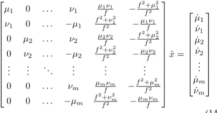
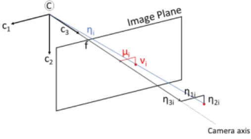
The detailed derivation of the OF formulae can be found in [8] here we only summarize the main equations. Fig. 1 shows the pinhole camera projection of a World point described by the following equation.
y= µi
νi
= f η3i
η1i
η2i
(1) where i = 1. . . m is the index of tracked feature points.
The number of tracked pointsmdepends on the field of view of the camera and the texture of the scenery.
Fig. 1: The mapping
The OF can be calculated by differentiating (1). This case we apply backward numerical differentiation (2)
˙
y(k) =y(k)−y(k−1)
∆t (2)
THIS IS THE AUTHOR VERSION OF ARTICLE PUBLISHED AT IEEE CNNA 2021 CONFERENCE 2
∆tequals the camera sample rate. According to [7] consid- ering the dynamics of the World point in the camera system because of A/C motion finally (3) can be constructed.
µ˙i
˙ νi
=
µi η3i −ηf
3i
0 νi µiνi
f −f2+µf 2i
νi
η3i 0 −ηf
3i
−µi
f2+νi2
f −µifνi
u v w p q r
(3)
Where [u, v, w],[p, q, r] are A/C velocity and angular rate vectors respectively,µi, νi are image feature coordinates,f is the camera focal length andη3i are the feature point distances along camera system c3 axis.
The vector of unknowns to be determined is:
x=
u v w p q r η31 . . . η3m
T
this givesm+ 6unknowns from2mequations. So at least 6 feature points are needed for a unique solution to exist. This is Method 1in [8] and leads to a high dimensional nonlinear optimization problem which does not fit low computational capacity.
A. Focus of Expansion Calculation
According to [8] the OF can be decoupled for translational and rotational components. The rotational is easily calculable knowing the angular rate of the A/C (4)
µ˙Ri
˙ νRi
=
"
νi µiνi
f −f2+µf 2i
−µi
f2+ν2i
f −µifνi
#
p q r
(4) The translational OF can be found by substracting the rotational part from the total OF.
µ˙T i
˙ νT i
=
µ˙i−µ˙Ri
˙ νi−ν˙Ri
(5) The Focus of Expansion (FOE) which is the direction of the A/C ground relative velocity vector in camera system can be found as the intersection of the lines resulting from the translational OF vectors as shown in Fig. 2.
Fig. 2: Translational optic flow radiates from the FOE (µF, νF) The constraint equation for the FOE results as (reorganizing equation (15) from [7] to avoid singularities)
˙
νTi(µi−µF)−µ˙Ti(νi−νF) = 0, ∀i (6) Considering all points this leads to the optimization:
µF νF
= arg min
(µ,ν)
1 2 C
µ ν
−d
2
(7) where
C=
−ν˙T1 −ν˙T2 . . . −ν˙Tm
˙
µT1 µ˙T2 . . . µ˙Tm
T
(8) and
d=
ν1µ˙T1−ν˙T1µ1 . . . νmµ˙Tm−ν˙TmµmT (9) This is a linear system of equations with 2 unknowns. Once the FOE is found, the ratio of the translational velocities can be obtained:
v u= µF
f , w u =νF
f (10)
[8] proposes a combination of (3) and (6) to remove the unknown η3i distances and get the angular velocity and the FOE together (namedMethod 3). This gives5unknowns from 2m equations but is also a nonlinear optimization problem:
J3i =
p q r
µ2i −µiµ+νi2−νiν
(µi−µ)(−νi2−f2)+(νi−ν)µiνi f
(µi−µ)µiνi−(νi−ν)(µ2i+f2) f
+
−(νi−ν) (µi−µ) µ˙i
˙ νi
≈0
(11)
(p, q, r, µF, νF) = arg min
(p,q,r,µ,ν) m
X
i=1
(J3i)2 (12) Meanwhile this optimization gives angular rates and FOE the accuracy of the latter can be improved by solving (7) based-on the estimated angular rates and a filtered set of points considering only the nearest ones according to [8].
However, from (12) one can not estimate the distance of the feature points as theη3i variables were removed so additional calculations are needed for feature selection
Considering the flaws of Method 1, Method 2 (low di- mensional but constrained nonlinear optimization, neglected here) and Method 3 from [8] our goal was to develop a computationally simpler method which is able to accurately estimate the angular rate, filter the feature points (near / far ones) and estimate FOE.
III. ANAPPROXIMATETWOSTEPLINEARSOLUTION
The idea behind this approach is that the A/C translational motion is dominated by the forward velocityu. We assume that v=w≈0. In this case we can alter the vector of unknowns:
ˆ x=h u
η31 . . . ηu
3m p q riT
(13) and get a linear system of equations from (3):
THIS IS THE AUTHOR VERSION OF ARTICLE PUBLISHED AT IEEE CNNA 2021 CONFERENCE 3
µ1 0 . . . ν1 µ1ν1
f −f2f+µ2 21
ν1 0 . . . −µ1 f2f+ν212 −µ1fν1 0 µ2 . . . ν2 µ2fν2 −f2f+µ2 22
0 ν2 . . . −µ2
f2+ν22
f2 −µ2fν2 ... ... . .. ... ... ... 0 0 . . . νm µmfνm −f2+µf22m
0 0 . . . −µm
f2+νm2
f2 −µmfνm
ˆ x=
˙ µ1
˙ ν1
˙ µ2
˙ ν2
...
˙ µm
˙ νm
(14) The solution givesp, q, r and an approximation of the ηu
3i
values as ηu∗
3i
. Introducing a correction factor foru, relatingv andw tou∗ and substituting into (3) gives:
ˆ xi= u∗
η3i
, u=cuu∗, v=cvu∗, w=cwu∗ (15)
µ˙i
˙ νi
=
"
µixˆi −fxˆi 0 νi µiνi
f −f2+µf 2i νixˆi 0 −fxˆi −µi
f2+µ2i
f −µifνi
#
cu
cv
cw
p q r
(16) which is again a linear problem and can give improved estimates for [p, q, r] and estimates for [u, v, w]/η3i. The angular rate estimates can be applied in (7)-based FOE calcu- lation possibly giving better results than calculating from the estimated velocity parameters.
IV. SIMPLETESTSIMULATIONS ANDRESULTS
The simple test simulations include the straight flight of an aircraft model in Matlab towards a grid of points defined in North-East-Down coordinates. Two point set surfaces are applied as summarized in Table I and shown in Fig. 3.
# N orth East Down
1 (−460 : 10 : 460)T (0 : 10 : 460)T −1.5yN ED+ 100 2 (−2300 : 100 : 2300)T (0 : 100 : 2300)T −0.2yN ED+ 0.1
TABLE I: Point set surface coordinates
Fig. 3: Visualized point set surfaces
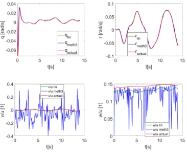
Fig. 4: Results in the 1st simulation
The starting position of A/C trajectory is (0,0,−277)T facing to the East. The end is at (−0.74,181.4,−276.95)T. The camera’s focal length is 2818.8px, the image plane is 4096×2160px. The simulation’s sample time is 0.02swhile the camera sample rate is 0.1s. Feature points inside the camera field-of-view are continuously tracked paying special attention to the ones visible in consecutive frames. Results from Method 3and the own approximate linearsolution are compared.
A. 1st simulation
The first simulation is run towards the closer surface (# 1).
Fig. 4 shows that the pitch rate is inaccurate with the linear method (the roll and yaw rates are accurate) and the pitch and yaw rates fromMethod 3are noisy. As the FOE calculation is very sensitive to the angular rates its results are not acceptable and so not presented.
B. 2nd simulation
In the second simulation the farther surface (# 2) is utilised.
It can be seen on the results in Fig. 5 that introducing points with larger depth (η3i) greatly improves the angular velocity estimates with both methods. The translational velocity ratios (obtained from FOE calculation with all points (2/A case)) with thelinearsolution are acceptable while in case ofMethod 3 the noisy pitch and yaw rate estimates generate high noise in the ratios. Note that the larger difference of the w/uratio from the actual value in case of thelinearmethod shows that thew≈0 assumption causes errors.
However, an advantage of the linear method is the possibil- ity to select the closest features from the ηu
3i
ratios. In the 2/B case we use this to get the closest 10 points, and calculate the FOE with both methods using only them. The translational velocity ratios in this case are shown in Fig. 6 with some improvement relative to the previous case.
Finally, the root mean square error (RMSE) of each param- eter with each method is calculated and summarized in Table II. It can be seen that the linear solutions are usually better than theMethod 3 results and choosing the closest points for FOE calculation improves the estimation with both methods.
The runtime of the two algorithms was compared in the Matlab script considering the 2nd simulation as there the number of tracked points as about the same (320−360) during the 14s flight time. Method 3 gave 25.31s while the linear method6.27sruntime so its much faster.
THIS IS THE AUTHOR VERSION OF ARTICLE PUBLISHED AT IEEE CNNA 2021 CONFERENCE 4
Fig. 5: Results in the 2/A simulation
Fig. 6: Results in the 2/B simulation
As a summary it can be stated that we have developed an approximate linear solution instead of the nonlinear ones which runs faster and gives equally good or better results.
RMSE 1st sim 2nd sim/A 2nd sim/B
lin meth3 lin meth3 lin meth3
perror 0.0039 0.0038 0.0037 0.0037 - - qerror 0.0080 0.0056 0.0037 0.0037 - - rerror 0.0014 0.0078 0.0024 0.0031 - -
v
u error 0.0168 0.1094 0.0033 0.1385 0.0027 0.1089
w
u error 0.0884 0.0527 0.0177 0.0429 0.0147 0.0273
TABLE II: RMSE of the translational velocity ratios
V. CONCLUSION
This paper targets the determination of aircraft angular rates and ground velocity vector direction from camera optical flow.
After the brief introduction of two existing nonlinear solution methods it introduces a new approximate linear solution con- sidering the dominance of the longitudinal aircraft velocity component. It is compared to the simplest nonlinear solution regarding precision and runtime in different simple simulated scenarios. It gave similar or better estimation accuracy with a significantly lower runtime. Thus future plans include its evaluation in more realistic conditions with synthetic and possibly real images.
REFERENCES
[1] Autonomous Systems National Laboratory. [Online]. Available:
https://autonom.nemzetilabor.hu/
[2] H.-P. Chiu, A. Das, P. Miller, S. Samarasekera, and R. Kumar, “Precise vision-aided aerial navigation,” in2014 IEEE/RSJ International Confer- ence on Intelligent Robots and Systems, 2014, pp. 688–695.
[3] G. Conte and P. Doherty, “An Integrated UAV Navigation System Based on Aerial Image Matching,” in2008 IEEE Aerospace Conference, 2008, pp. 1–10.
[4] ——, “Vision-Based Unmanned Aerial Vehicle Navigation Using Geo- Referenced Information,” EURASIP Journal on Advances in Signal Processing, vol. 2009, no. 1, p. 387308, Jun. 2009. [Online]. Available:
https://doi.org/10.1155/2009/387308
[5] D. Dusha, W. Boles, and R. Walker, “Attitude Estimation for a Fixed- Wing Aircraft Using Horizon Detection and Optical Flow,” in 9th Biennial Conference of the Australian Pattern Recognition Society on Digital Image Computing Techniques and Applications (DICTA 2007), 2007, pp. 485–492.
[6] D. Dusha, L. Mejias, and R. Walker, “Fixed-wing attitude estimation using temporal tracking of the horizon and optical flow,” Journal of Field Robotics, vol. 28, no. 3, pp. 355–372, 2011. [Online]. Available:
https://onlinelibrary.wiley.com/doi/abs/10.1002/rob.20387
[7] J. Kehoe, R. Causey, A. Arvai, and R. Lind, “Partial aircraft state estimation from optical flow using non-model-based optimization,” in 2006 American Control Conference, 2006, pp. 6 pp.–.
[8] J. Kehoe, A. Watkins, R. Causey, and R. Lind, “State Estimation Using Optical Flow from Parallax-Weighted Feature Tracking,” in In Proc. of AIAA Guidance, Navigation, and Control Conference and Exhibit, ser. Guidance, Navigation, and Control and Co-located Conferences. American Institute of Aeronautics and Astronautics, Aug. 2006. [Online]. Available: https://doi.org/10.2514/6.2006-6721 [9] P. Roberts, R. Walker, and P. O’Shea, “Tightly Coupled GNSS and
Vision Navigation for Unmanned Air Vehicle Applications,” in New Opportunities through International Partnering: Proceedings of the Eleventh Australian International Aerospace Congress, M. Scott, Ed.
Australia: Institution of Engineers, Australia and Royal Aeronautical Society, Australian Division, 2005, pp. 1–22. [Online]. Available:
https://eprints.qut.edu.au/2877/
[10] B. Simlinger and G. Ducard, “Vision-based Gyroscope Fault Detection for UAVs,” in2019 IEEE Sensors Applications Symposium (SAS), 2019, pp. 1–6.
[11] J. Woo, K. Son, T. Li, G. S. Kim, and I. Kweon, “Vision-based UAV Navigation in Mountain Area,” inProceedings of the IAPR Conference on Machine Vision Applications (IAPR MVA 2007), May 16-18, 2007, Tokyo, Japan, 2007, pp. 236–239. [Online]. Available: http://b2.cvl.iis.u- tokyo.ac.jp/mva/proceedings/2007CD/papers/08-03.pdf
![Fig. 2: Translational optic flow radiates from the FOE (µ F , ν F ) The constraint equation for the FOE results as (reorganizing equation (15) from [7] to avoid singularities)](https://thumb-eu.123doks.com/thumbv2/9dokorg/758404.32717/2.918.468.846.84.357/translational-radiates-constraint-equation-results-reorganizing-equation-singularities.webp)