Estimating river nutrient concentrations consistent with good ecological condition: More stringent nutrient thresholds needed

(1)

Ecological Indicators 121 (2021) 107017

Available online 30 November 2020

Estimating river nutrient concentrations consistent with good ecological condition: More stringent nutrient thresholds needed

Sandra Poikane

^a^,^*

, G ´ abor V ´ arbír o ´

^b

, Martyn G. Kelly

^c^,^d

, Sebastian Birk

^e^,^f

, Geoff Phillips

^g

aEuropean Commission, Joint Research Centre (JRC), I-21027 Ispra, Italy

bDepartment of Tisza Research, Danube Research Institute, Centre for Ecological Research, Bem t´er 18/c, H-4026 Debrecen, Hungary

cBowburn Consultancy, 11 Monteigne Drive, Bowburn, urham, DH6 5QB, UK

dDepartment of Geography, Nottingham University, Nottingham, NG7 2RD, UK

eUniversity of Duisburg-Essen, Faculty of Biology, Aquatic Ecology, Universit¨atsstrasse 5, 45141 Essen, Germany

fUniversity of Duisburg-Essen, Centre for Water and Environmental Research, Universit¨atsstrasse 5, 45141 Essen, Germany

gSchool of Biological and Environmental Sciences, University of Stirling, Stirling, FK9 4LA, UK

A R T I C L E I N F O Keywords:

Eutrophication Ecological status Phosphorus Nitrogen Rivers Nutrient targets

A B S T R A C T

Nutrient pollution remains one of the leading causes of river degradation, making it important to set thresholds that support good ecological condition, which is the main objective of managing Europe’s aquatic environment.

A wide range of methods has been used by European member states to set river nutrient thresholds in the past, and these vary greatly among countries, even for similar river types. In some countries, thresholds have been set using expert judgement or the statistical distribution of nutrient concentrations. Application of such thresholds creates problems for planning strategies to achieve good ecological status and for managing transboundary river basins. An alternative approach is to examine the statistical relationship between nutrient concentration and one, or more, biological variables. Such relationships can then be used to inform decisions by water managers. We use such ’ecology-based’ approaches (univariate regression and mismatch analyses) to derive nutrient thresholds for several river types in Central Europe. Our analysis focused on soluble reactive phosphorus (SRP) and total nitrogen (TN), two variables which were responsible for significant variation (40–55%) in river benthic floras. In this study, for the first time, river nutrient thresholds are estimated using both macrophytes and phytobenthos (EQRs) separately and in combination, calculated as the minimum and the average of the EQRs of the two sub- elements. The resulting thresholds supporting good ecological status range from 21 to 42 µg/L SRP and 0.9–3.5 mg/L TN for the low alkalinity lowland river type, and 32–90 µg/L SRP and 1.0–2.5 mg/L TN for the low alkalinity mid-altitude river type. These targets are compared to the values set by member states. We demon- strate that some national nutrient thresholds fall within the range of predicted values if uncertainty is taken into consideration; however, several threshold values considerably exceed this range. Adopting ecology-based nutrient targets should improve sustainable river management where nutrients are the major pressure pre- venting the achievement of good ecological status.

1. Introduction

Although rivers are critical for providing provisioning (water and food), regulating (water purification, climate resilience) and cultural (recreation and tourism) ecosystem services, they are facing unprece- dented threats from urbanization, agriculture and climate change (MEA, 2005; V¨orosmarty et al., 2010; Reid et al., 2019) and are heavily ¨

degraded throughout Europe. A recent analysis has shown that less than half (42%) of river stretches in Europe are in high and good ecological status, with the remainder divided between moderate (36%), poor and bad (17%) or unknown (5%) (EEA, 2018). Several pressures affect Eu- ropean rivers, often simultaneously: hydrological and morphological alteration, chemical contamination, microplastics, overexploitation and alien species (Schinegger et al., 2012; Grizzetti et al., 2017; Birk et al.,

Abbreviations: BQE, Biological Quality Element; EQR, Ecological Quality Ratio; SRP, soluble reactive phosphorus; TP, total phosphorus; TN, total nitrogen; WFD, Water Framework Directive.

* Corresponding author.

E-mail address: sandra.poikane@ec.europa.eu (S. Poikane).

Contents lists available at ScienceDirect

Ecological Indicators

journal homepage: www.elsevier.com/locate/ecolind

https://doi.org/10.1016/j.ecolind.2020.107017

Received 14 April 2020; Received in revised form 21 September 2020; Accepted 26 September 2020

(2)

2020). The effects are further exacerbated by climate change (Charlton et al., 2018). However, nutrient pollution remains one of the leading causes of river degradation (EEA, 2018; Carvalho et al., 2019). The consequences of nutrient enrichment include increased algal and macrophyte biomass, changed dissolved oxygen and pH regimes, changes in composition and abundance of biological communities and food webs, and altered rates of nutrient and carbon cycling (Dodds and Welch, 2000; Hilton et al., 2006). These effects have major impacts on the delivery of ecosystem services and entail high economic costs (e.g.

increases in water treatment costs and degradation of recreational op- portunities; McDonald et al., 2016; Grizzetti et al., 2019).

The last decades have seen huge advances in aquatic ecological assessment. The Water Framework Directive (WFD, 2000/60/EC) has been a major driver for this in Europe, requiring assessment of four Biological Quality Elements (BQEs) in rivers (benthic flora, benthic in- vertebrates, fish fauna and, in large rivers with high retention time, phytoplankton). One hundred and forty river assessment methods have been intercalibrated (i.e. compared and harmonized) and included in the monitoring programs of European countries (Kelly et al., 2009;

Poikane et al., 2014, 2020). One half of the methods are based on primary producers and target nutrient enrichment: macrophytes (e.g., Haury et al., 2006), phytobenthos (e.g., V´arbír´o et al., 2012), and phytoplankton (e.g., Mischke et al., 2011).

However, although ecological assessment is crucial, it is only a first step toward reaching good status. Once the causes of ecological degradation have been identified, it is then necessary to set management targets for good ecological status and implement a remediation program. Recent reviews of the WFD implementation have identified problems in these later stages (Carvalho et al., 2019).

A potential solution to this difficult problem could involve (i) establishing causal links between stressors and appropriate biological variables. If the stressor of interest is a nutrient, then plant-based BQEs that respond directly to increased nutrients are most relevant to address, rather than higher trophic levels; and, (ii) establishing scientifically sound empirically-based management targets, such as setting nutrient concentrations consistent with good ecological status. Many different approaches have been proposed for setting nutrient targets, ranging from whole-population and reference-population percentiles (Chambers et al., 2008) to linking nutrient targets to predetermined biological outcomes (e.g., phytobenthos biomass; Dodds et al., 1997) and identifying a change point in the nutrient pressure-response models (Smith and Tran, 2010). However, each of these approaches has its own shortfalls, often associated with subjective factors embedded in each of them (Wang et al., 2007; Chambers et al., 2012).

Recently, technical guidance has been developed to enable countries to establish or review thresholds for phosphorus and nitrogen to support good ecological status (Phillips et al., 2018). This guidance describes

statistical methods for determining concentrations appropriate to support ecological status and facilitates the establishment of comparable and consistent boundaries across all European member states. So far, this approach has been applied to lakes (Poikane et al., 2019a), coastal and transitional waters (Salas Herrero et al., 2019) and to synthetic datasets, in order to elucidate the most appropriate approaches under different conditions (Phillips et al., 2019). However, recent analysis revealed that the biggest problems are associated with rivers (Poikane et al., 2019b). A wide range of methods has been used by countries to set river nutrient thresholds, and, consequently, these thresholds are highly variable among countries, even in rivers of a similar type. In some countries, thresholds were set using expert judgement or statistical distributions of nutrient concentrations with no consideration of ecological status. Such nutrient criteria create problems for planning strategies to achieve good ecological status and for managing transboundary river basins.

To date, the problem of setting river nutrient thresholds consistent with good ecological status has received scant attention in the research literature and there has been no investigation of nutrient targets for transnational rivers in Europe. Therefore, the aims of this study are to:

• explore relationships between nutrients and nutrient sensitive-BQEs in rivers of the Central-Baltic ecoregion of Europe;

• derive nutrient thresholds consistent with good ecological status where possible; and,

• compare the thresholds with the nutrient boundaries in use by countries and to discuss the implications of chosen thresholds.

In addition, we provide a comprehensive overview of ecologically- derived nutrient thresholds in rivers that could be useful when setting nutrient targets.

2. Material and methods 2.1. Data

We used data from the Central-Baltic region of Europe, which were collated for the intercalibration of biological assessment methods (Table 1). As required by the WFD, European member states established biological assessment methods for macrophytes and phytobenthos in rivers (Birk et al., 2012). National assessments are expressed as Ecological Quality Ratios (EQR), calculated as a ratio between observed and expected (at reference conditions) metric values, ranging from 1 (near-natural condition) to 0 (the worst possible ecological condition).

At first, high-good and good-moderate class boundaries are established by countries following the WFD normative definitions (Annex V, 1.2), afterwards they are intercalibrated and harmonized between countries Table 1

Summary of datasets used for deriving relationships and nutrient thresholds. SRP =soluble reactive phosphorus; TP =total phosphorus; TN =total nitrogen. The river types are specified in Table 2.

River type code Number of samples: Macrophytes Number of samples: Phytobenthos Range of values and [median]

SRP TP TN SRP TP TN SRP (µg/L) TP (µg/L) TN (mg/L)

R-C1 247 369 263 120 79 100 4-421 [28] 10-1400 [140] 0.04-14.6 [2.02]

R-C3 128 366 58 230 67 58 1-370 [40] 4-580 [66] 0.03-4.6 [0.624]

R-C4 432 129 334 436 81 304 1-3440 [66] 3-1460 [160] 0.2-15.5 [1.98]

R-C6 82 82 – 120 82 – 10-1600 [192] 3-1900 [240] –

Table 2

Description of Central-Baltic ecoregion shared river types (Bennett et al., 2011).

River type Type code Catchment area (km²) Altitude (m a.s.l.) Alkalinity (meq/L) Channel substrate, bank width

Small low alkalinity lowland R-C1 10–100 <200 <1.0 Sand, 3–8 m

Small low alkalinity midaltitude R-C3 10–100 200–800 <0.4 Boulders, cobbles and gravel, 2–10 m

Medium-sized mixed alkalinity lowland R-C4 100–1000 <200 >0.4 Gravel and sand, 8–25 m

Small lowland calcareous R-C6 10–300 <200 >2.0 Gravel, 3–10 m

(3)

in order to ensure that the boundaries are consistent across the EU (Kelly et al., 2009; Birk and Willby, 2010; Poikane et al., 2014). The biological data used in this study were normalised national EQR values (i.e. status class boundaries adjusted to 0.8, 0.6, 0.4 and 0.2; for a detailed description of the normalization procedure, see EC, 2011 (p.78) and Moe et al., 2015). National datasets were grouped into WFD intercalibration common river types, defined by their basin size, altitude, dominant geology, alkalinity and substrate (Table 2).

We examined the nutrients: total phosphorus (TP), soluble reactive phosphorus (SRP) and total nitrogen (TN). Sampling frequencies ranged from single (spot) to annual means based on monthly measurements.

Austria provided 90^thpercentile values; these were halved before being included in the analysis.

A variety of approaches have been adopted for macrophyte assessment (Table 3), all of them including an index of the sensitivity of macrophytes to nutrient enrichment, i.e. the average score of indicative species weighted by their abundance and, in some cases, also the taxon‘s ecological tolerance (Haury et al., 2006; Szoszkiewicz et al., 2006a;

Willby et al., 2012). In addition to sensitivity measures, there are several country-specific metrics. The Dutch method includes a metric for the abundance of growth forms (Pot and Birk, 2015), while the UK method includes richness of macrophyte growth forms, macrophyte taxa richness and cover of green filamentous algae (Willby et al., 2012). All indices are directed at eutrophication and significant relationships with nutrients (Birk and Willby, 2010; Birk et al., 2012). Most countries use a measure of phytobenthos (Table 3), with diatom indices based on a weighted-average approach and optimized against gradients of nutrients (Rott et al., 1997, 1999; Kelly et al., 2008) or general degradation (Coste, in CEMAGREF, 1982). An exception is the Dutch index EKR, which is based on proportions of positive and negative diatom indicator taxa (Van der Molen, 2004).

2.2 Methods for estimating nutrient threshold supporting good ecological status

Technical guidance has been developed that describes statistical methods for determining appropriate concentrations to support good ecological status along with a toolkit (Phillips et al., 2018), which pro- vides the statistical models in the form of R scripts (R Core Team, 2019).

We selected two approaches described in this guidance, following the experiences gained by testing different approaches with synthetic datasets (Phillips et al., 2019):

1) Univariate linear regression between EQR and nutrient concentrations, with nutrient threshold values predicted by the regression models. Type II regression (Ranged Major Axis regression; RMA) was used, which assumes equal uncertainty in measurement of both EQR and nutrients. Segmented regression methods were used to test for linearity within the data set.

2) The ‘minimization-of-mismatch’ approach determines the nutrient concentration that gives the lowest mismatch between classification based on biology and on nutrient concentration. The boundaries predicted by our analysis were compared with the boundaries set by countries (for overview and details see Poikane et al., 2019a).

In addition to estimating nutrient thresholds for macrophytes and phytobenthos separately, the average and minimum of the EQRs of the Table 3

Description of member states macrophyte and phytobenthos assessment methods.

Country/

biological quality element

The name of the method Reference

Macrophytes

Denmark Danish Stream Plant Index (DSPI) Søndergaard et al., 2013

Luxembourg Biological Macrophyte Index for

Rivers (IBMR) Haury et al., 2006

Netherlands Revised assessment method for rivers in The Netherlands using macrophytes (includes species

Pot and Birk, 2015 composition metrics and growth

forms abundance metrics) Poland Polish Macrophyte Index for Rivers

(MIR) Szoszkiewicz et al.,

2006b UK Ecological Classification of Rivers

using Macrophytes LEAFPACS2 (includes River Macrophyte Nutrient Index, Number of functional groups, Number of macrophyte taxa, and Filamentous algal cover)

Willby et al., 2012

Phytobenthos

Austria Multimetric Index (including Trophic index, Saprobic index and Reference index)

Pfister and Pipp, 2010 Luxembourg Indice de Polluosensibilit´e

Sp´ecifique (IPS) Coste, in CEMAGREF, 1982

Netherlands EKR (Ecologische Kwaliteitsratio) based on proportions of positive and negative indicator taxa

Van der Molen, 2004 Poland Diatom Index for rivers (Avg of

Trophic index and Saprobic index) Pici´nska-Fałtynowicz, 2009; Rott et al., 1997, 1999

UK Revised Trophic Diatom Index

(TDI) Kelly et al., 2008

Table 4

Coefficients of determination (r²) resulting from linear regression analysis between nutrients, Biological Quality Elements, and their combinations. Relationships used for setting of the nutrient thresholds are given in bold. TP =total phosphorus; SRP =soluble reactive phosphorus; TN =total nitrogen; n.s. =relationship non- significant.

River type Nutrient Macrophytes Phytobenthos Macrophytes and

phytobenthos combined (avg)

Macrophytes and phytobenthos combined (min)

R-C1 TP 0.00 (n.s.) 0.20** 0.03 (n.s.) 0.04 (n.s.)

SRP 0.41** 0.42** 0.49** 0.48**

TN 0.40** 0.49** 0.55** 0.65**

R-C3 TP 0.09** 0.14** 0.15* 0.11**

SRP 0.40** 0.43** 0.48** 0.54**

TN 0.49** 0.53** 0.46** 0.48**

R-C4 SRP 0.18** 0.06** 0.22** 0.27**

TP 0.00 0.01 (n.s) 0.00 0.01 (n.s)

TN 0.09** 0.03* 0.08** 0.08**

R-C6 TP 0.08** 0.10** 0.18** 0.12**

SRP 0.02 (n.s.) 0.00 0.11** 0.04 (n.s.)

* p <0.05; ** p <0.01

(4)

two organism groups were used.

3. Results 3.1. Relationships

In low alkalinity streams (R-C1 and R-C3), SRP and TN were strongly related to macrophyte and phytobenthos assessments (both singly and in combination). The relationship with TP was weaker or non-significant, as was the relationship to nutrients in higher alkalinity types. We therefore did not pursue the threshold analysis for this nutrient parameter and these types (Table 4).

3.2. Univariate regression models

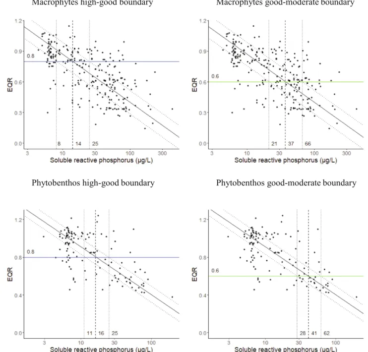
For low alkalinity lowland rivers (R-C1), the relationship between SRP and Macrophyte EQR predicted a concentration for the good- moderate boundary of 37 µg/L, with 50% of the data having values between 21 and 66 µg/L (Fig. 1). Results for the high-good boundary were 14 (range 8–25) µg/L SRP. The univariate relationships between SRP and phytobenthos predicted a good-moderate threshold of 41 µg/L SRP (range: 28–62 µg/L) and high-good threshold of 16 µg/L SRP (range:

11–25 µg/L) (Fig. 1). The results for the R-C3 type is included in the Supplementary material.

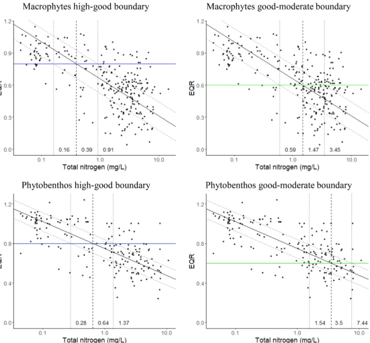
The relationships between TN and macrophytes predicted a good- moderate threshold of 1.47 mg/L with a range of 0.59–3.45 mg/L and high-good threshold of 0.39 (range: 0.16–0.91) mg/L TN.

Macrophytes high-good boundary Macrophytes good-moderate boundary

Phytobenthos high-good boundary Phytobenthos good-moderate boundary

Fig. 1. Relationship between Ecological Quality Ratios (EQR) for macrophytes (upper block) and phytobenthos (lower block) with soluble reactive phosphorus for low alkalinity lowland rivers (Type R-C1) showing high-good boundary (left) and good-moderate boundary (right) values. Solid line shows type II RMA regression, dotted lines show area containing 50% of the data.

(5)

Relationships for TN and phytobenthos produced a good-moderate threshold of 3.5 mg/L (range: 1.54–7.44 mg/L) (Fig. 2). The high- good criteria were 0.64 mg/L TN (range: 0.28–1.37) mg/L.

The combined macrophyte/phytobenthos models (calculated as the minimum of the EQRs of the two organism groups) gave the most stringent predictions: good-moderate criteria of 32 µg/L SRP (range:

18–58 µg/L) and 1.63 mg/L TN (range: 0.71–4.19 mg/L) (Fig. 3).

The results for both river types and all BQEs are summarised in Table 5 and 6.

3.3. Minimise the mismatch between classifications based on biology and nutrient concentration

For the R-C1 type using macrophytes, the values for good-moderate thresholds were 42 µg/L SRP and 2.21 mg/L TN (Fig. 4), while the high- good class thresholds were 19 µg/L SRP and 0.85 mg/L TN. For the phytobenthos assessment the good-moderate thresholds were at 32 µg/L

SRP and 2.86 mg/L TN (Tables 5 and 6).

3.4. Comparison with nutrient boundaries in use by countries

For SRP, countries have set good-moderate class boundaries ranging from 90 to 100 µg/L SRP for R-C1 and 70 to 130 µg/L SRP for R-C3, expressed as annual mean or vegetation season mean (Phillips and Pitt, 2016). Thresholds expressed as annual 90^thpercentile equal to 160 µg/L SRP for R-C1 and 20–160 µg/L SRP for R-C3.

For TN, countries have set good-moderate boundaries ranging from 2.3 to 10.0 mg/L for R-C1, similar values (i.e. 2.0–10.0 mg/L) for the R- C3 type, expressed as annual mean or vegetation season mean (Poikane et al., 2019b; Phillips and Pitt, 2016).

A comparison with our results (Table 5 and 6) shows the following:

• Several of the reported boundary values are within the range of the predicted values (e.g., 70 µg/L SRP or 2 mg/L TN);

Fig. 2. Relationship between Ecological Quality Ratios (EQR) for macrophytes (upper block) and phytobenthos (lower block) with total nitrogen for low alkalinity lowland rivers (Type R-C1) showing high-good boundary (left) and good-moderate boundary (right) values. Solid line shows type II RMA regression, dotted lines show area containing 50% of the data.

(6)

•However, some of these boundary values exceed this range significantly (e.g., 130 µg/L SRP or 10 mg/L TN);

•There is a particularly strong difference for the R-C1 type and SRP values where all values set by countries (90–100 µg/L SRP) are considerably higher than SRP values supporting good ecological status established by our analysis (21–42 µg/L SRP).

4. Discussion

4.1. Setting nutrient thresholds in rivers

Nutrient enrichment may adversely affect both structure and func- tion of stream ecosystems. Therefore, river ecologists and managers need to identify nutrient thresholds that will ensure risks of ecological impairment are low. In this study, we used relationships between

nutrient-sensitive organism groups (macrophytes and phytobenthos) and nutrient concentrations to identify nutrient thresholds consistent with good ecological status. The most robust relationships were found for SRP and TN in low alkalinity rivers explaining 40–55% of variance.

The resulting thresholds range from 21 to 42 µg/L SRP and from 0.9 to 3.5 mg/L TN for the low alkalinity lowland river type, and from 32 to 90 µg/L SRP and from 1.0 to 2.5 mg/L TN for the low alkalinity mid-altitude river type.

There are many ways to estimate nutrient threshold levels in rivers.

The most common methods include (i) the percentiles approach, e.g.

using the 25^thpercentile of the whole-population (which assumes that the best available values are appropriate) or 75^thpercentile of reference sites (Stevenson et al., 2008); (ii) approaches based on ecological effects of nutrients to the river ecosystem (Smucker et al., 2013). The percentile approach has been criticized for disregarding ecological response and Fig. 3. Relationship between combined macrophyte and phytobenthos Ecological Quality Ratios (EQR) (minimum) with soluble reactive phosphorus (upper block) and total nitrogen (lower block) for low alkalinity lowland rivers (Type R-C1) showing high-good boundary (left) and good-moderate boundary (right) values. Solid line shows type II RMA regression, dotted lines show area containing 50% of the data.

(7)

providing over- or underprotective criteria which might mislead river managers (Chambers et al., 2012; Smucker et al., 2013). In contrast, criteria based on ecological effects provide information on nitrogen and phosphorus concentrations associated with low ecological impairment (Hausmann et al., 2016; Charles et al., 2019) and serve as benchmarks for assessing and managing water resources.

The ecology-based approaches fall in two categories: (i) linking nutrient concentrations to a predefined ecological condition (typically, a certain level of the benthic algal biomass or composition-based metric, Chambers et al., 2012; Dodds and Welch, 2000, Charles et al., 2019), and (ii) identifying a change-point in the relationships between nutrients and biological variables (Smith and Tran, 2010; Stevenson et al., 2008; Tibby et al., 2019). However, these two approaches both have drawbacks. Using the first approach, the nutrient threshold will depend on the choice of biological variable and on the definition of acceptable limits. For benthic chlorophyll-a concentrations, for instance, acceptable limits range from 50 to 200 mg/m²(Chambers et al., 2012), leading to large differences in corresponding nutrient thresholds (Dodds and Welch, 2000). The change-point approach seems to be more objective;

however, the result depends on (i) the analytical approach employed, as the threshold values can differ depending on the choice of statistical method (e.g. non-parametric change-point analysis, regression tree analysis or other; Wang et al., 2007; Smucker et al., 2013) and (ii) biological communities and variables used for analysis (Wang et al., 2007; 2008; Zheng et al., 2008; Chen et al., 2018). In addition, more than one change-point might be identified in some relationships (Ste- venson et al., 2008; Smucker et al., 2013), creating a dilemma about the choice of the right threshold. Also, the change-point identified might be located at the very beginning or at the higher end of the nutrient

gradient. For instance, Stevenson et al. (2008) found TP thresholds between 10 and 12 µg/L TP; however, these levels coincide with reference conditions, so protection of all streams with this threshold was deemed impractical.

We followed the former approach in this study, primarily because the WFD requires member states to set thresholds in order to support good ecological status. The main advantage of this approach is that ecological status boundaries are set according to WFD definitions and then harmonised amongst EU member states to give a consistent framework for setting ecologically-meaningful nutrient thresholds.

We found that thresholds differed depending upon whether phytobenthos, macrophytes or a combination was used (Table 4). Differences between thresholds obtained using macrophytes and phytobenthos may occur because they have access to different pools of nutrients (water and/or sediment) and also because they respond at different rates to changes in the nutrient concentration. In theory, the organism group most sensitive to phosphorus should be used, but model strength also needs to be taken into account, as well as a recognition of their different contributions to ecosystem processes. Models that use both macrophytes and phytobenthos are stronger than those that use one or the other. Kelly et al. (2020) recommend the use of the average of the two organism groups rather than the minimum, as this approach incorporates information from both organism groups toward the final threshold.

4.2. Relationships between phytobenthos and macrophyte communities and nutrients in rivers

Pressure-response relationships describe the effect of different levels of pressure (nutrients in this case) on components of an ecosystem and Table 5

Summary of predicted soluble phosphorus (SRP) high-good and good-moderate class boundaries (µg/L) for low alkalinity lowland rivers (R-C1) and low alkalinity upland rivers (R-C3). The table includes the values predicted by the linear regression model (in brackets: range defined as 25^thand 75^thpercentiles of the residuals of the linear model). For the mismatch analyses the nutrient concentration is shown that yielded the lowest mismatch between classifications based on biology and nutrient concentration (in brackets: the 25^thand 75^thpercentiles of cross-over values calculated from the bootstrap (n =500) replicates).

River type Method used Macrophytes Phytobenthos Macrophytes and

phytobenthos (average)

Macrophytes and phytobenthos (minimum) High-good class boundary

R-C1 Linear regression 14 (8–25) 16 (11–25) 12 (7–21) 10 (6–18)

Mismatch 19 (17–22) 13 (11–15) 11 (10–13) 9 (8–9)

Mismatch 14 (12–18) 20 (16–23) 18 (15–25) 9 (7–11)

Good-moderate class boundary

Mismatch 42 (37–49) 32 (24–42) 26 (22–30) 21 (17–28)

Mismatch 70 (50–95) 70 (59–87) 81 (62–98) 32 (28–38)

Table 6

Summary of predicted total nitrogen (TN) high-good and good-moderate class boundaries (mg/L) for low alkalinity lowland rivers (R-C1) and low alkalinity upland rivers (R-C3). See Table 5 for further explanation.

River type Method used Macrophytes Phytobenthos Macrophytes and

phytobenthos (average)

Macrophytes and phytobenthos (minimum) High-good boundary

RC-1 Linear regression 0.39 (0.16–0.91) 0.64 (0.28–1.37) 0.36 (0.18–0.68) 0.22 (0.10–0.57)

Mismatch 0.85 (0.61–1.05) 0.71 (0.62–0.83) 0.72 (0.60–0.91) 0.26 (0.20–0.31)

R-C3 Linear regression 0.50 (0.24–1.05) 0.84 (0.43–1.73) 0.70 (0.4–1.7) 0.38 (0.22–0.85)

Mismatch 0.51 (0.40–0.66) 0.94 (0.78–1.11) 0.60 (0.50–0.80) 0.40 (0.34–0.47)

Good-moderate class boundary

Mismatch 2.21 (1.80–2.40) 2.86 (2.30–3.12) 1.76 (1.500–2.00) 0.90 (0.60–1.10)

Mismatch 1.80 (1.30–2.30) 1.72 (1.44–1.89 1.80 (1.40–2.30) 1.04 (0.96–1.12)

(8)

can be used to identify thresholds associated with good ecological condition (Stevenson et al., 2008; Chambers et al., 2012). However, such models tend to have low explanatory power, especially in rivers due to a looser coupling of ecological response to nutrient loading in rivers, than in lakes. The difference between lotic and lentic response is due to a number of factors: physical controls - channel morphology and substrate, flow velocity, flow regime, and light availability (including riparian shading and turbidity) (Dodds et al., 2002; Hilton et al., 2006).

In this study, we found moderately strong relationships between nutrients (SRP, TN) and primary producers (macrophytes and phytobenthos) in low alkalinity streams R-C1 and R-C3 (r²=0.40–0.65, p <

0.001, Table 4) while the relationship with TP in these stream types was weak (r²=0.09–0.20, p <0.001) or non-detectable. In all other river types, characterized by higher alkalinity, relationships between primary producers and all nutrients (SRP, TP and TN) were weak (r²= 0.03–0.27, p <0.001) or non-detectable.

Benthic algae play a central role in river eutrophication assessment because of their importance to primary production and strong links to nutrient concentrations (Potapova and Charles, 2007; Smucker et al., 2013; Poikane et al., 2016). Many studies have established relationships between nutrients and phytobenthos metrics (Table 7). However, studies have found that indices based on species composition, particularly diatom trophic indices, are more strongly linked to nutrients than

biomass or diversity (Porter et al., 2008; Stevenson et al., 2008). The relationship between algal biomass and nutrient concentration is com- plex, as it is strongly shaped by other factors, such as current velocity, turbidity, riparian shading, grazing and scouring by floods (Biggs, 2000;

Dodds et al., 2002; Stevenson et al., 2006, 2008). For these reasons, diatom composition metrics are the most widely-used phytobenthos variables, also included in our study (Table 3). In general, studies have demonstrated variable results ranging from very weak to strong relationships (Table 7). The range in sensitivity could result from a number of issues: First, diatom composition metrics are calibrated against different gradients depending on the study. For example, some are calibrated to nutrients (e.g. TDI: Kelly et al., 2008), while others are calibrated to general degradation (e.g. IPS, Coste in CEMAGREF, 1982).

The latter, whilst often including some correlation with nutrient concentrations, will also reflect other stressors. Both types, in addition, are influenced by natural gradients unrelated to nutrients, particularly current velocity, turbidity (Soininen, 2005) and alkalinity (Kelly et al., 2008; Lavoie et al., 2014). Similarly, metrics such as the TDI are usually calibrated against phosphorus concentration. Stoichiometric calcula- tions generally suggest phosphorus, rather than nitrogen, is more likely to be the limiting nutrient. Therefore, questions need to be asked about the validity of using such metrics for setting nitrogen thresholds. In re- ality, nitrogen and phosphorus concentrations are often correlated Fig. 4. Percentage of water bodies at low alkalinity lowland rivers (Type R-C1) where either the macrophyte assessments or soluble reactive phosphorus classifications for good ecological status differ in comparison to the level used to set the high-good boundary (left) and good-moderate boundary (right). Vertical lines mark the intersection of curves where mis-match is minimized and equal.

(9)

(Kelly et al., 2020) and, whilst this might be helpful for deriving nitrogen concentrations associated with good ecological status, it does not necessarily mean that there is a causal relationship.

Macrophytes respond not only to nutrient concentrations in the water, but also to sediment nutrients, shading, hydrological conditions and substrate (Szoszkiewicz et al., 2006b; Wiegleb et al., 2016). In addition, other anthropogenic pressures such as hydrological alteration, herbicide application, and weed-cutting practices may have consider- able effect on macrophyte communities (Baattrup-Pedersen et al., 2002, 2003). For these reasons, establishing direct links between macrophyte communities and nutrients has been problematic. Therefore, different approaches have been used, for instance, relationships to land-use metrics (Kuhar et al., 2011), composite pressure gradients (Aguiar et al., 2011; Dodkins et al., 2012) or simple categorical comparisons between impacted and non-impacted sites (Aguiar et al., 2009).

While many studies have tried to establish pressure-response relationships (Table 8), these studies have primarily used macrophyte composition indices that claim to detect nutrient pollution, such as the macrophyte Mean Trophic Rank (Holmes et al., 1999) or IBMR (Haury et al., 2006). Only a few studies attempt to establish relationships with abundance measures (Willby et al., 2012) and these are typically weaker than relationships with composition metrics. The strength of macrophyte-nutrient relationships range from weak or non-significant to moderately strong (up to r²=0.48–0.56; Willby et al., 2012). In our study, strong relationships were observed (explaining 41 to 49% of the biological variance) whilst in high or mixed alkalinity streams the explained variance was lower (8 to 18%).

The use of dissolved versus total nutrient forms has generated much discussion, with no clear conclusions (Dodds et al., 1997; Dodds and Welch, 2000; Hilton et al., 2006; Wagenhoff et al., 2017). Some studies Table 7

Relationships between phytobenthos variables and nutrients. TP =Total phosphorus; SRP =Soluble reactive phosphorus; TN =Total nitrogen; SIN =Soluble inorganic nitrogen; NO3 =Nitrate; TON =Total organic nitrogen; n.s. =not significant.

Reference Biological metric vs nutrient

metric Coefficient of

determination (r²) Phytobenthos abundance

Biggs, 2000 (New

Zealand) Mean/max benthic chl-a vs

SRP 0.23/0.29

Mean/max benthic chl-a vs SIN 0.12/0.32 Chambers et al.,

2008 (Ontario and Quebec, Canada)

Benthic chl-a TN 0.46

Benthic chl-a TP n.s.

Chambers et al., 2012 (Ontario and Quebec, Canada)

Benthic chl-a vs TP 0.15 Benthic chl-a vs TN 0.45 Ch´etelat et al., 1999

(Ontario and Quebec, Canada)

Benthic chl-a vs TP 0.56 Benthic chl-a vs TN 0.50

Cladophora biomass vs TP 0.53

Melosira biomass vs TP 0.64

Demars et al., 2012

(Eastern England) Abundance of filamentous

algae vs SRP 0.08

Dodds et al., 1997 (N. America and New Zealand)

Mean/max benthic chl-a vs TP 0.09 / 0.07 Mean /max benthic chl-a vs

SRP 0.05 / n.s.

Mean / max benthic chl-a vs

TN 0.35 / 0.28

Dodds et al., 2002 (National Stream Water-Quality Monitoring)

Benthic chl-a vs TP 0.03 Benthic chl-a vs TN 0.06 Benthic chl-a vs NO3 0.08 Smucker et al., 2013

(Connecticut, US) Benthic chl-a NO2+3 (NOx) 0.14

Benthic chl-a TP 0.1

Stevenson et al., 2006 (North- Central region, US)

Benthic chl-a vs TP 0.04–0.17 Benthic chl-a vs TN 0.07–0.19

Cladophora cover vs TP 0.12–0.45

Cladophora cover vs TN 0.08–0.30

Stevenson et al., 2008 (Mid-Atlantic Highlands region, US)

Benthic chl-a vs TP n.s.

Algal ash-free dry mass vs TP 0.04

Willby et al., 2012

(United Kingdom) Algal cover vs SRP 0.06 Algal cover vs TON 0.05 Benthic chl-a vs TN 0.07–0.19

Cladophora cover vs TP 0.12–0.45

Cladophora cover vs TN 0.08–0.30

Stevenson et al., 2008 (Mid-Atlantic Highlands region, US)

Benthic chl-a vs TP n.s.

Algal ash-free dry mass vs TP 0.04

Willby et al., 2012

(United Kingdom) Algal cover vs SRP 0.06 Algal cover vs TON 0.05 Diatom trophic and diversity metrics

Almeida et al., 2014 (Mediterranean region)

ICM (IPS and TI) vs TP 0.18 ICM (IPS and TI) vs SRP 0.37 ICM (IPS and TI) vs NO3 0.06 Chambers et al.,

2012 (Ontario and Quebec, Canada)

Diatom metrics vs TP 0.40–0.43 Diatom metrics vs TN n.s.

Diatom diversity metrics vs TP n.s.

Diatom diversity metrics vs TN 0.17 Hlúbikov´a et al.,

2007 (Slovakia) Diatom indices vs TP 0.27–0.37 Diatom indices vs TN 0.30–0.34 Kelly and Whitton,

1995 (UK) Trophic diatom index (TDI) vs

SRP 0.63

Kelly et al., 2008

(UK) Trophic diatom index (TDI) vs

SRP 0.35

Trophic diatom index (TDI) vs NO3

0.29 Lavoie et al., 2008

(Eastern Canada) Eastern Canadian Diatom

Index (IDEC) vs TP 0.41–0.79 Lavoie et al., 2014

(Eastern Canada) IDEC vs TP 0.35

Porter et al., 2008 Diatom indices vs TP 0.04–0.32 Diatom indices vs SRP 0.03–0.25

Table 7 (continued)

determination (r²) Diatom indices vs TN 0.02–0.28 Potapova and

Charles, 2007 High/Low-P indicators vs TP 0.27–0.56 High/Low-N indicators vs TN 0.16–0.73 Rott et al., 2003

(Austria) Austrian Trophic Index vs TP 0.72 Smith and Tran,

2010 (New Yourk state, US)

Diatom metrics vs TP 0.03–0.5 Diatom metrics vs TN 0.02–0.43 Diatom metrics vs TP 0.01–0.25 Smucker and Vis,

2009 (Ohio, US) Diatom similarity metrics vs

SRP 0.18–0.19

Diatom similarity metrics vs NO3

n.s.

High/Low-P indicators vs SRP n.s.

High/Low-P indicators vs NO3 0.10 High/Low-N indicators vs SRP 0.14 High/Low-N indicators vs NO3 0.13 Smucker et al., 2013

(Connecticut, US) Diatom metrics vs NO2+3

(NOx) 0.16–0.42

Diatom metrics vs TP 0.31–0.55 Stevenson et al.,

2008 (Mid-Atlantic Highlands region, US)

Diatom diversity metrics vs TP 0.10 Diatom metrics vs TP 0.05–0.33

V´arbír´o et al., 2012

(Hungary) Diatom indices vs SRP 0.40

Diatom indices vs TN 0.034–0.35 Vilbaste et al., 2007

(Estonia) Diatom indices: IPS vs SRP 0.12–0.18

IBD vs SRP 0.13–0.20

IPS vs TN 0.18

IBD vs TN n.s.

IPS and IBD vs NO3 n.s.

IBD vs NO3 n.s.

Zheng et al., 2008

(West Virginia, US) Diatom indices vs TP 0.17–0.22 Diatom indices vs NOx 0.46–0.55 Diatom diversity indices vs TP 0.02 Diatom diversity indices vs

NOx 0.06–0.09

(10)

(Dodds et al., 1997; Porter et al., 2008) have found that relationships were generally stronger for total than for dissolved nutrient concentrations. However, several models based on dissolved concentrations of nutrients have been successful (Kelly and Whitton, 1995; Biggs, 2000;

Willby et al., 2012), and some studies have found stronger relationships with dissolved than with total nutrients (Taylor et al., 2004; Zheng et al., 2008; Fabris et al., 2009; Almeida et al., 2014). In our study, we found strong relationships with SRP, while the relationships with TP were weaker or non-significant. Two explanations (not mutually exclusive) can be put forward to explain these results: (i) limited P bioavailability (Mainstone and Parr, 2002; Hilton et al., 2006; Charles et al., 2019) and (ii) naive nutrient sampling regimes (Hilton et al., 2006; Jarvie et al., 2006; Lavoie et al., 2008). However, we lack the data to test these hy- potheses in the present work.

Similarly, weaker relationships were found in high alkalinity streams. We hypothesize that this was due to over-riding influence of Table 8

Relationships between macrophytes variables and nutrients. TP =Total phosphorus; SRP =Soluble reactive phosphorus; TN =Total nitrogen; NO3 =Nitrate;

TON =Total organic nitrogen.

determination (r²) Macrophytes trophic indices

Aguiar et al., 2011 (Portugal,

western Iberia) Mean Trophic Rank (MTR) vs SRP, NO3

0.12–0.16 MTR vs TP, TN 0.09–0.12 Riparian vegetation index

(RVI) vs TP, TN, SRP 0.09–0.12 Demars et al., 2012 (North-

east France, Eastern England)

Macrophyte Biological Index for Rivers (IBMR) vs SRP 0.32 IBMR vs SRP (after

removing the effects of pH) 0.08

IBMR vs NO3 0.002

River macrophyte nutrient index (RMNI) vs SRP and bioavailable P in sediments

n.s.

Demars and Harper, 1998

(England) Mean Trophic Rank (MTR)

vs SRP 0.34

MTR vs NO3 0.18

Fabris et al., 2009 (Germany) Reference index (RI) vs SRP 0.18

RI vs TP 0.05

Trophic index of

Macrophytes (TIM) vs SRP 0.41

TIM vs TP 0.21

Flor-Arnau et al., 2015

(Spain) Macrophyte Fluvial Index

(IMF) vs SRP 0.19

IMF vs NO3 0.20

Su´arez et al., 2005 (Spain) Index of macrophytes (IM)

vs SRP 0.16

IM vs NO3 n.s.

Szoszkiewicz et al., 2006a

(Europe) IBMR vs TP 0.16–0.49

IBMR vs SRP

MTR vs TP 0.23–0.59

MTR vs SRP 0.27–0.67

MTR vs NO3 0.06–0.48

Willby et al., 2012 (United

Kingdom) RMNI vs SRP 0.48

RMNI vs TON 0.58

Macrophyte abundance metrics Szoszkiewicz et al., 2006a

(Europe) Cover Bryophytes vs TP

(mountain streams) 0.37 Cover Bryophytes vs SRP (mountain streams) 0.38 Cover Bryophytes vs NO3

(South-European sites) 0.35 Cover Floating free vs SRP (mountain streams) 0.18 Willby et al., 2012 (United

Kingdom) Total cover vs SRP 0.028

Total cover vs TON 0.040 Invasive species cover vs

SRP 0.012

Invasive species cover vs

TON 0.006

Table 9

Nutrient thresholds set by different ecology-based methods. BCG =Biological Condition Gradient; TIN = Total Inorganic Nitrogen; NMS = Non-metric Multidimensional Scaling; TITAN = Threshold Indicator Taxa ANalysis. See Table 7 for other abbreviations.

Reference Nutrient

criteria Approach to setting criteria Benthic (or sestonic) algae abundance

Carleton et al., 2009

(Minnesota, US) 100 µg/L TP;

2.7 mg/L TN Threshold to prevent nuisance levels of periphyton and cyanobacteria dominance in sestonic algae Chambers et al., 2008

(Ontario, Canada) (1) 1.8 mg/L TN; (2) 21 µg/L TP; 0.95 µg/L TN

(1) Benthic chl-a <100 mg/m² (2) Sestonic chl-a <5 mg/L;

Predictions from linear regressions

Chambers et al., 2012

(Ontario, Canada) (1) 1.2 mg/L TN; (2) 14 mg/L TP

(1) Benthic chl-a <100 mg/m²; (2) Sestonic chl-a <5 mg/L;

Predictions from linear regressions Dodds et al., 1997

(Montana, US) 30 µg/L TP;

0.35 mg/L TN

Thresholds to control nuisance benthic chl-a levels <100 mg/m²;

Regression and probabilistic analyses Dodds and Welch, 2000

(US) 60 µg/L TP;

0.47 mg/L TN

Thresholds to control mean benthic chl-a levels <100 mg/m² Dodds et al., 2002, 2006

(US) 43–62 µg/L

TP; 0.54–0.60 mg/L TN

Break-points in nutrient–benthic chl-a regressions (mean and max chl-a)

Miltner, 2010

(Ohio, US) 38 µg/L TP;

0.44 mg/L DIN

Change point in nutrient-benthic chl-a relationship

Royer et al., 2007

(Illinois, US) 70 µg/L TP Sestonic chl-a <5 mg/L Stevenson et al., 2006

(Kentucky, Indiana and Michigan regions, US)

30 µg/L TP;

1.0 mg/L TN Threshold indicating high probabilities (20–50%) of extensive Cladophora growths (>20% avg.

cover) Wong and Clark, 1976

(Ontario, Canada) 60 μ_{g/L TP} Threshold to limit excessive seasonal growth of Cladophora

Diatom composition Chambers et al., 2012

(Ontario, Canada) 22–32 µg/L TP; 0.59 mg/L TN

Thresholds in pressure-response of diatom metrics identified by regression tree analysis Charles et al., 2019

(New Jersey, US) 50 µg/L TP;

1.0 mg/L TN Threshold between impaired and unimpaired sites (BCG 4.0) based on diatom taxonomic composition;

Visual graph analysis Hausmann et al., 2016

(Wadeable streams in the US)

50 µg/L TP Threshold between impaired and unimpaired sites (BCG 3.7) based on diatom taxonomic composition;

TITAN Lavoie et al., 2008

(Quebec, Canada) 20–40 µg/L

TP Diatom index IDEC values show a significant drop

Smith and Tran, 2010 (Large rivers of New York State, US)

(1) 9–20 µg/

L TP;

0.41–0.50 mg/L TN (2) 37 µg/L TP; 0.78 mg/L TN

Thresholds shifts in biological community;

(1) change points analysis;

(2) cluster analysis

Smucker et al., 2013

(Connecticut, US) (1) 20 μ_g/L TP; (2) 40 μ_g/L TP; (3) 65 μg/L TP

(1) Sensitive taxa steeply decline;

(2) Diatom community change-points above which most sensitive diatoms lost; TITAN and NMS

Stevenson et al., 2008 (Mid-Atlantic Highlands)

10–20 µg/L

TP Thresholds in Lowess regression and regression tree analysis

Tibby et al., 2019

(South Australia) 30 µg/L TP Threshold indicating significant decline in sensitive diatom species;

TITAN Benthic invertebrate fauna

(continued on next page)

(11)

alkalinity and that inclusion of alkalinity in the model might provide a better solution (Kelly et al., 2008; Demars et al., 2012; Lavoie et al., 2014).

4.3. Nutrient threshold values in rivers

There is a growing body of research efforts worldwide to understand the effects of nutrients on river ecology and to derive ecology-based nutrient thresholds (Table 9). A wide variety of thresholds has been suggested, subject to the biological community and variables used in the analyses, as well as the method applied to set the threshold. The type of river also plays an important role although only a few studies have considered river type when setting thresholds. Despite the differences, some common patterns do emerge: Most studies point to a TP threshold of about 30 to 60 µg/L TP, above which algal biomass may reach nuisance levels and diatom composition changes significantly. There are fewer studies on TN thresholds, and they are more variable, yet most studies converge around a TN threshold of 0.5–2.0 mg/L. For example, Hausmann et al. (2016) defined 52 µg/L TP as a change-point in diatom assemblages, while Tibby et al. (2019) identified thresholds of impairment in Australian watersheds at 30 µg/L TP and Lavoie et al. (2008) at 20–40 µg/L TP in Canadian streams. Similarly, thresholds of 30 µg/L TP and 1.0 mg/L TN were proposed by Stevenson et al. (2006) and 50 µg/L TP and 1.0 mg/L TN by Charles et al. (2019), both based on the response in benthic algal community. Smith and Tran (2010) provide more

conservative guidelines of 37 µg/L TP and 0.7 mg/L TN, based on shifts in biological community structure of benthic macroinvertebrate and diatoms. Similar values (i.e., 30 µg/L TP and 0.35 mg/L TN) are given by Dodds et al. (1997) to control nuisance benthic algal levels, while Chambers et al. (2008, 2012) identify TN thresholds for excessive benthic algal biomass at 1.2 and 1.8 mg/L TN.

These values coincide with the nitrogen planetary boundary values of 1.0–2.5 mg/L N derived to protect aquatic ecosystems from eutrophication or acidification (de Vries et al., 2013). A concentration of 100 µg/L SRP is often quoted as the point above which few changes to the phytobenthos or macrophytes occur (Bowes et al., 2007; Mainstone, 2010) but detailed studies nearly always indicate that significant changes have already occurred before this threshold is reached (Table 9). Our work provided nutrient thresholds in a range of 30–90 µg/

L SRP and 1–3.5 mg/L TN, which were broadly comparable with these previous studies.

Comparison with the nutrient limits set by countries sharing these river types shows that several national nutrient thresholds are too high and will not protect sites from becoming ecologically impaired. These thresholds, therefore, need to be revisited. It is not surprising as a recent analysis demonstrated that a large variety of methods has been used for boundary setting, and the boundaries set by expert judgement tend to be higher (=less strict) than those set using contemporary data from the region in question (Poikane et al., 2019b).

5. Conclusions

If water bodies are to achieve good ecological status, establishing scientifically sound nutrient thresholds is of great importance. Exami- nation of pressure-response relationships provide an objective method for establishing nutrient concentration thresholds in support of good ecological status. Our study demonstrates that in some cases it is possible to link nutrient concentrations to assessments of macrophyte and phytobenthos communities for determining nutrient thresholds.

However, in other cases the explained variance was low, and further work is needed to consider the effect of other natural and anthropogenic stressors, as well as the nutrient sampling regime.

Finally, comparison of our nutrient thresholds with those used by selected EU member states showed that some states currently use thresholds that are too high. These high thresholds fail to protect rivers from becoming ecologically impaired and require examination and revision.

CRediT authorship contribution statement

Sandra Poikane: Conceptualization, Methodology, Data curation, Writing - original draft, Supervision, Project administration. G´abor Varbír´ o: ´ Conceptualization, Methodology, Software, Formal analysis, Investigation, Data curation, Visualization. Martyn G. Kelly: Concep- tualization, Methodology, Data curation, Writing - original draft.

Sebastian Birk: Conceptualization, Methodology, Writing - original draft. Geoff Phillips: Conceptualization, Methodology, Software, Formal analysis, Investigation, Data curation, Writing - original draft, Visualization.

Declaration of Competing Interest

The authors declare that they have no known competing financial interests or personal relationships that could have appeared to influence the work reported in this paper.

Acknowledgements

This work was carried out under the WFD Common Implementation Strategy working group ECOSTAT work program. We greatly acknowl- edge the contributions of the ECOSTAT representatives and national Table 9 (continued)

Reference Nutrient

criteria Approach to setting criteria Chambers et al., 2012

(Ontario, Canada) 21–63 µg/L TP; 0.59–2.83 mg/L TN

Thresholds in pressure-response of benthic fauna metrics identified by regression tree analysis Chen et al., 2018

(North-east China) 52–101 µg /L TP; 1.05–1.65 mg/L TN

Breakpoints in the response of benthic invertebrate metrics;

Regression tree analysis and Lowess Smith et al., 2007

(Wadeable rivers of New York State, US)

65 µg/L TP;

0.98 mg/L NO3

Threshold between impaired and unimpaired sites; Cluster analysis Smith and Tran, 2010

(Large rivers of New York State, US)

(1) 11–70 µg/L TP;

0.5–1.2 mg/

L TN;

(2) 37 µg/L TP; 0.68 mg/L TN

Thresholds shifts in biological community:

(1) Change points analysis;

(2) Cluster analysis

Wang et al., 2007

(Wisconsin, US) 40–90 µg/L TP; 0.61–1.68 mg/L TN

Threshold at which benthic invertebrate metrics change most dramatically to small changes in nutrient levels; Regression tree analyses

Weigel and Robertson, 2007

(Wisconsin, US)

64–150 µg/L TP; 0.64–1.93 mg/L TN

Breakpoints in nutrient-response relationships; Regression tree analysis

Fish fauna

Miltner and Rankin, 1998

(Ohio, US) 60 µg/L TP;

0.61 mg/L TIN

Threshold beyond which fish community structure is likely to be significantly degraded (based on IBI index)

Wang et al., 2007 (Wadeable streams of Wisconsin, US)

60–90 µg/L TP; 0.54–1.83 mg/L TN

Threshold at which fish metrics change most dramatically to small changes in nutrient levels; Regression tree analyses

Weigel and Robertson, 2007

(Wisconsin, US)

91–139 µg/L TP; 0.64 mg/L TN

Breakpoints in nutrient-response relationships; Regression tree analysis