Graph Models of Neurodynamics
to Support Oscillatory Associative Memories
Gabriel P. Andrade∗, Mikl´os Ruszink´o†, Robert Kozma∗‡
∗College of Information and Computer Sciences University of Massachusetts Amherst, 140 Governors Drive
Amherst, MA 01003, USA
†Alfr´ed R´enyi Institute of Mathematics, Hungarian Academy of Sciences 13-15 Re´altanoda utca, H-1053 Budapest, Hungary
‡Department of Mathematical Sciences, University of Memphis 373 Dunn Hall, Memphis, TN 38152, USA
Email: andrade@math.umass.edu∗, ruszinko.miklos@renyi.mta.hu†, rkozma@cs.umass.edu‡
Abstract—Recent advances in brain imaging techniques re- quire the development of advanced models of brain networks and graphs. Previous work on percolation on lattices and random graphs demonstrated emergent dynamical regimes, including zero- and non-zero fixed points, and limit cycle oscillations. Here we introduce graph processes using lattices with excitatory and inhibitory nodes, and study conditions leading to spatio-temporal oscillations. Rigorous mathematical analysis provides insights on the possible dynamics and, of particular concern to this work, conditions producing cycles with very long periods. A systematic parameter study demonstrates the presence of phase transitions between various regimes, including oscillations with emergent metastable patterns. We studied the impact of external stimuli on the dynamic patterns, which can be used for encoding and recall in robust associative memories.
Index Terms—Graph Theory, Percolation, Cellular Automata, Associative Memory, Neurodynamics.
I. INTRODUCTION
Advanced brain monitoring techniques provide us with ever more detailed experimental insights into spatial-temporal brain activity [1]–[4]. Much of what is found can be understood rig- orously using dynamical systems theory and there is evidence that the brain is a high-dimensional, complex chaotic system being perturbed by stimuli to produce collective behaviors [5], [6]. In the presence of input stimuli, the degrees of freedom temporarily collapse, and the brain undergoes a transition into an ordered phase, while the system effectively exists in a lower dimensional sub-space. When the input is removed, the brain returns to its high-dimensional, chaotic trajectory while wan- dering through phase space. This leads to the cinematic theory of brain dynamics, which is defined through a sequence of phase transitions between chaos and order [2], [7]. Regardless of one’s commitment to specific brain models, it is clear that the brain is some kind of dynamical system. Accordingly, individual tasks performed by brains should follow dynamical principles; this means learning and memory functions can be viewed as manifestations of dynamical associative memories.
Designing associative memory models as dynamical sys- tems has been extensively studied. The most popular and best understood of these models diverge from the insights
just mentioned in that they encode memories as fixed point attractors of the system [8], [9]. These models are being initialized in a state specified by the input and converge to the nearest point attractor. This approach fails to account for the fact that brains display non-random neural activity in the absence of input [1], [10], [11] and that this activity is likely to influence how the input perturbs the system [12]. In addition to these fixed-point memory schemes, significant work has been done on memories based on bifurcations and limit cycles of neural dynamical systems [13], [14]. These models maintain activity in the absence of input and produce promising results, which have the potential to be more efficient memories [14], and benefit from insights gained from the extensive work on neurodynamics. These models still rely on classical dynamical systems and ordinary differential equations (ODEs), which have inherent numerical problems when implemented on a computer. These problems are exacerbated by the complex interactions inherent in any system with associative memory;
not only is finding solutions to the nonlinear ODEs being used time consuming and imprecise, but these problems are snow- balled by the complicated multifaceted relations necessarily learned by a system having associative memory.
We introduce a simple neural model with properties that are promising for use in neural associative memories while avoiding the shortcomings mentioned above. This model ex- hibits self-sustained dynamics ranging from fixed points to unpredictable oscillations that still can be reliably controlled.
Furthermore, the model is a deterministic graph process which makes it well suited to being modeled on a computer without worries of numerical error. We begin by defining the model and its dynamic process. This is followed by reviewing previ- ous work on this approach and a brief analysis of the model’s dynamics under different parametrizations. We discuss how the model can be controlled in the absence of stimuli and give preliminary results on the effects external stimuli have when applied to this system. We conclude with a discussion of future work and directions of how this model could be used to build associative memories.
II. MODELDESCRIPTION
A. The Graph(E, I)
In this paper we will consider the neural network (E, I).
This neural network can be constructed as a graph consisting of an excitatory layer E and an inhibitory layer I. The excitatory layer of the network,E, is defined as theZ2 lattice over a(N)×(N)grid with periodic boundary conditions (i.e. a torusT2= (Z/NZ)2). In other words,Eis a graph consisting ofN2vertices that each are only adjacent to four neighbors. In a more general problem setting, motivated by the long axonal connections in the neural tissue, we introduced a random graph model Gwith edges e(G), that consists of a square grid and additional random edges [15]. The definition of the model captures an important property of cortical networks, that is, it is more likely for a neuron to have connections to nearby neurons than to neurons which are far from the given one.
The random edges of the graph are distance-dependent, i.e., the probability that an arbitrary pair of vertices,u, v, that are at distance dapart of each other, is given by
pd=P((u, v)∈e(G)|dist(u, v) =d) = c
N dα, (1) where d > 1, c is a positive constant, and α is the power exponent of long edge length distribution. It is assumed that there are no multiple edges between the vertices. In this work, we do not consider random additional edges, i.e., c = 0, for simplicity.
We define the inhibitory layer, I, as the complete graph KN2
4
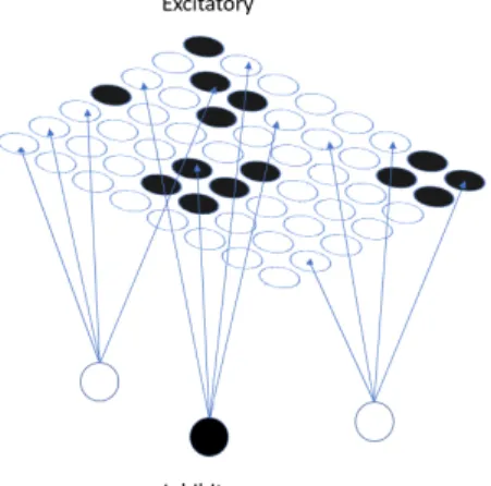
with the additional property that each vertex is connected to four excitatory vertices in E at random in such a way that no two inhibitory nodes share any excitatory neighbors. This is to say thatIcomprises of N42 vertices that are each adjacent to every other vertex in I and also to four excitatory vertices in E that no other inhibitory vertex is adjacent to. When we consider these layers together we have the network(E, I) as can be seen in Figure 1. It is worth noting that by V(E)and V(I) we are denoting the the set of nodes in the excitatory and inhibitory layers respectively.
B. Spiking Process in (E, I)
Each node in both E andI can take on one of two states:
active or inactive. Let χv(t)define the potential function for node v in either layer at timet such that χv(t) = 1 if v is active and χv(t) = 0 if v is inactive at time t. The state of a node is completely determined at every time step by the state of itself and its neighbors in the previous time step.
To define this formally, let AE(t) denote the set of active vertices in E at time t and similarlyAI(t)denote the set of active inhibitors at time t. Furthermore, define AE(0) as a random subset of excitatory nodes that became active based on a Bernoulli process with probabilitypinover the excitatory vertices and AI(0) = ∅. Then for a vertex in E we say its state at time t+ 1is
χv(t+ 1) =1
X
u∈N(v)∩V(E)
χu(t)≥k
Similarly, for a vertex inI we have
χv(t+ 1) =1
X
u∈N(v)∩V(E)
χu(t)≥`
In both cases1is the indicator function andN(v)denotes the subset of nodes in the closed neighborhood ofv(i.e the nodev and its neighbors). Bothkand`are nonnegative integers that specify the number of active neighbors any given vertex needs to become active on the next time step inEandIrespectively.
Finally we introduce the inhibitory firing function that enables spiking behavior on(E, I). This firing function causes all of the inhibitors to fire together oncem∈[0,N42]inhibitory vertices are active during a time step. In other words, an inhibitory nodev∈V(I)fires at timet+ 1if
Fv(t+ 1) =1
X
u∈N(v);u,v∈V(I)
χu(t)≥m
butv did not fire at timet. Notice that active inhibitory nodes fire simultaneously since they are in all to all connection with one another. At the time of firing, an inhibitory vertex sets its own activity and the activity of all excitatory vertices adjacent to it to 0. This is to say that in a firing step the following vertices become inactive: (i) all inhibitory nodes, and (ii) those excitatory nodes which were connected to an active inhibitory node that was firing at that step. After the inhibitory firing occurs both layers carry on by propagating activity (or the lack thereof) with whichever excitatory nodes were left active. We will refer to this time between one inhibitory firing and the next as a spike. NB: This use of the word spikeis different from the typical use inspiking neural networks; however, for simplicity we keep this terminology.
Fig. 1: Example of(E, I). Circles depicted in black are active vertices in either E or I. Note that we do not show all inhibitory vertices inI for the sake of clarity.
As was briefly mentioned above, the excitatory layer E of this network is a special case of percolation. These percola- tion models have been studied extensively and and are well
understood in the case when the potential function’s parameter k = 2. In [15], [16] it is shown that assuming there is no inhibition (or m > N42), when k = 2 in the excitatory node’s activation rule,Ehas an asymptotic critical probability pc = 0 (i.e. if vertices in E are activated with arbitrarily small positive probability, it will become fully active with probability approaching1as the size ofEapproaches infinity).
Therefore there always exists a system large enough such that for any pin > 0, regardless of how arbitrarily small, with high probability (whp) all of the vertices in Ewill eventually become active when the inhibitors are not allowed to fire.
III. RESULTS
By coupling E andI and introducing the inhibitory firing rule, cyclic behavior becomes a near guarantee with the right parameters. By choosing parameters in such a way that the firing process extinguishes vertices while maintaining
|AE|
N2 > pc in the specified network, whp the activation in both layers begins growing once more until the next firing and we obtain sustained spiking behavior. We aim to control this interesting oscillatory behavior demonstrated by(E, I)to model emergent associative memory. This necessitates that we show this network can reliably exhibit identifiable dynamics under certain conditions and that these conditions are easily reproducible yet robust. In the concluding remarks we shall briefly discuss how we can tune our parameters in a way that allows input to influence the dynamics by allowing these conditions to be met.
We begin by introducing some results about the general network(E, I)withk= 2so that we gain some insight on the effect that the other parameters have on the network’s behavior.
Using the parametrization that this analysis indicates is most suited for our task we show the effects of different m on the oscillatory behavior. Finally, we demonstrate some results of this graph process when stimuli in the form of perturbations are introduced.
A. Effects of Parameters on Network Dynamics
Due to the work on percolation mentioned above and because of results we’ve obtained that are outside the scope of this paper, during the remainder of our discussion it should be assumed k = 2. We explore the behavior of the network when N2, `, m, and pin are left general. By considering the effect that the inhibitory firing rule has on the excitatory layer’s activity we uncover sufficient conditions for firing.
Proposition 1: Given a network (E, I), ` = 1, . . . ,4, and m∈[0,N42].
1) If|AE(t)|> N2−(5−`)(N42−m+ 1)then the system will necessarily fire
2) If `m≤ |AE(t)| ≤N2−(5−`)(N42 −m+ 1)then the system has the potential to fire
3) and if |AE(t)|< `mthen the system will not fire.
Due to space constraints, we do not give here the com- plete proof; interested readers are referred to an online ver- sion through BINDS web server https://binds.cs.umass.edu;
DARPA Report, Year 1, Task 3. Properties(1)and(2)in this proposition suggests that there exists some excitatory activa- tion density, |ANE2|, in the range[`m, N2−(5−`)(N42−m+1)]
where the system will fire with near certainty. By making the naive assumption that at any time,t, the probability of a node inE being active is independent of all other nodes and instead dictated by a Bernoulli trial with success parameter described by the actual excitatory activation density, we find that this simplified model has a probability of firing that is dictated by the sum of Binomial distributions. Furthermore because this assumption simply reduces the inhibitory firing to a function of the excitatory activation density, firing in the actual model implies firing in the simplified system but not the inverse direction. As such, by considering the limit as the size of the system approaches infinity we find that for each` andm there is an excitatory activation density in [`m, N2−(5−`)(N42 −m+ 1)]where the system will fire whp. Call this densityphighc . From this we find that
Corollary 1:For every fixed `, and N the network (E, I) cannot display oscillatory dynamics for m such that `m >
phighc .
Our discussion thus far makes clear that higher values of
` make oscillatory behavior a possibility in a wider range of parameter space. On top of this we see that when ` is held fixed, the parametermalmost exclusively influences the possible length of spikes in the network. Consider now the initialization density parameter pin. We find that aside from the first spike,pinhas no effect on the length spikes.
Proposition 2: For every fixed ` = 1, . . . ,4 and positive integerN, as time increases, the spike length in the oscillatory region of parameter space depends on the density of active inhibitory vertices needed to fire (4mN2) but does not depend on initialization probability pin.
Just as for Proposition 1, we do not give here the complete proof for the sake of space; interested readers are referred to an online version; see comment after Proposition 1. Intuitively this phenomenon makes sense because, regardless of how densely the system in initialized if we have chosen parameters that allow for oscillatory dynamics, then once the inhibitors fire and activity needs to build again the network “forgets” the state it was in prior to firing and behaves similarly to a system initialized at its newAE(t).
These results are all demonstrated in Figure 2 whenN2= 10000, ` = 4, and k = 2. This plot contains in each com- bination of m and pin a simulation of the system initialized at random using these parameters. We stepped through every m ∈ [0,2500] and through pin ∈ [0,1]with steps of 0.001, each time recording the length of the most recent spike after 1000time steps. Note thatphighc is less than the absolute upper bound mentioned above in property(1)of Proposition1, that there is a sharp cut-off of oscillatory behavior whenmis large enough, and that spike length is invariant on pin. Figure 2 also acts to present the one caveat to Proposition2that is not made clear without us presenting the proof. That is to say,pin does not influence spike length unless pin happens to cause
the system to propagate activity in a way that leads |ANE2| to become significantly larger than phighc forcing the inhibitory firing to bring the system below the critical probability. As can also be seen in Figure 2, this is only actually a concern for a very small window of possible pin.
Fig. 2: A heat map capturing log2 of the most recent spike’s length after 1000time steps. The network has N2 = 10000,
`= 4, andk= 2.
B. Oscillatory behavior When k= 2 &`= 4
Thus far we have spoken of the spiking process only in the abstract, but by considering the properties above in tandem with our empirical results we begin to see the choice of parameters necessary to produce the oscillatory behavior we desire for the largest possible range of m, for any sized network. For the remainder of this paper let k = 2, ` = 4, and pin> pc in such a way that it doesn’t cause the system to grow too fast before the first spike. Furthermore, in all preceding figuresN2= 10000and the simulations are run for at least1000000time steps. With these parameters established, we will explore the oscillatory dynamics we are interested in specifically. It should be clear that our system qualitatively exhibits two type of behavior: either the network becomes stuck at a fixed point or it oscillates.
This network’s oscillatory behavior is particularly promising for modeling associative memory because, through numerous experiments, we have noticed that not all oscillations seem to be the same. Formless than around1750our network(E, I) seems to exhibit perfectly periodic behavior with the number of unique spikes in a a period increasing proportionally with m for most random mappings of the inhibitory vertices to the excitatory vertices. When m is greater than around1750 something happens and suddenly, for most random mappings of the inhibitory vertices to the excitatory vertices the system does not exhibit clear periodic behavior for over 10 million time steps. These periods are so long that if this were not a finite network with finite states, we might conclude this was a chaotic regime. To ensure that this was not some short lived phenomena we fixed an initialization and ran simulations of the network with every value ofmfor10000,50000,100000,
1000000, and10000000time steps. For each of these spans of time we kept track of how manym did not display periodic behavior by the end, we did a linear fit of this data, and found that if this trend continues there will be certain values ofm that do not fall into a period for a hundred trillion time steps.
Thus we can safely conclude that this erratic spiking behavior is not born of some transient.
Interestingly, the transition from simple to erratic dynamics is gradual inmup untilmis too large to allow for oscillations.
Figure 3 captures this transition from a simple fixed point at very low values ofm, to periodic spiking, to the unpredictable spiking atm greater than around 1750, and finally into fixed points of activity below pc when m is too large. This figure is produced by plotting the last 10000 excitatory activation densities |ANE2|, at eachm, that the network had for a simulation initialized with the same seed each time. Therefore we can see different stages of a spike in the gaps in they-axis and if the network is periodic it will plot multiple points on top of one another. In this way we are able to get a visual sense of how erratic the spiking is at eachm based on how unable we are to discern individual steps taken by the excitatory layer of the network.
Fig. 3: A plot of the reset parameter min the x-axis and at each value of m we plot the last10000 excitatory activation densities attained by the network. We can see a transition in the dynamics of (E, I) from simple, to incredibly complex, and back to simple.
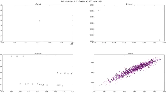
Though Figure 3 is a good visual aide for extracting the qualitative information we have mentioned, it lacks the specificity to allow us to discern a period with multiple spikes within it and the erratic spiking. This is in part because the dimensionality of (E, I) grows quickly with the size, N2, of the network. We attempt to combat this by reconstructing the attractor using a time-embedding delay and then taking a Poincar´e section of the resultant vectors. Due to the fact that (E, I) does not travel through phase space in a smooth nor continuous way the guarantees normally associated with both techniques do not apply, but by reconciling different embedding horizons we are able gain many insights. Figure
?? gives us a side by side comparison of embedding the time series {|AE(t)| : t ∈ [950000,10000000]} into three dimensional space, treating the resultant vectors as if they
were a form of step function in phase space, and taking a Poincar´e section for a period with a single spike in it, two spikes, twenty four spikes, and finally erratic spiking (i.e.
m= 600,1180,1550,1860).
We can now more clearly see the difference in these dynamic regimes. Notice that the1-period appears as1 point, a 2-periodic point appears as 2 points, and so on. This visualization already makes rather clear that the erratic spikes differ tremendously from typical periodic spiking, but it gives us no information about local activity in either E norI. For this reason, in exchange for simplicity and clarity, we capture some of the spatial information of the active vertices in E.
To do this we designated a node as the “center” and took a weighted sum of the active vertices in such a way that a node’s weight exponentially decays with distance from the
“center” node. This has the benefit of producing a map at each time step of E’s spatial activity that is unique up to certain symmetries about the “center” point, but suffers from the fact that nodes which are further away from this “center”
contribute so little that for larger networks it is smaller than machine epsilon. That being said in Figure??we plot the three dimensional time-embedding delay of this newly introduced excitatory activation time series. To help us establish a notion of orientation, which is not intuitive since we are treating time as a spatial dimension, we have colored the edges in the figure based on which time axis is firing from one moment to the next. The color corresponding to each direction is in the legend at the top of the figure.
With Figure ??, we are now able to see features which were obscured by the sheer number of points being plotted per m in Figure 3. Most striking is the fact that the embedding delay for every m, especially the erratic spiking, shows us that essentially all of the spikes in a period are of the same length. We see this in the fact that points being plotted near one another spike along the same axes as is most notably demonstrated by the thick colored bands in the embedding of the erratic spiking time series in Figure ??.
We have now shown that (E, I), under proper parameter- ization, exhibits an interesting form of complexity where it clearly does not have trivial oscillatory dynamics but is also not quite as unpredictable and unruly as a truly chaotic system.
The presence of this complexity is seen in Figures 3 and ??
while the regularities of the dynamics are put on display in Figure ??. We further reinforce both of these observations in the recurrence plots of our time-embedding delays in Figure 6.
These plots are created by disregarding the unintuitive spatial behavior of our network to instead focus on the temporal features of what we have seen so far. Define the time series in the time-embedding delays as
x(t) =
|AE(t)|,|AE(t+τ)|, . . . ,|AE(t+nτ)|
:t∈T
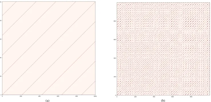
Then in Figure 6 we see plotted(t, t0), wheretandt0 are any
two time steps, whenever||x(t)|| ≈ ||x(t0)||1. In Figure 6a we see a recurrence plot for m = 1550 which has 24 spikes in a period while in Figure 6b we have the plot form = 1860 which has erratic spiking; both show us the last 50000 time steps of a 10000000time step simulation of(E, I).
We lose all information about where in a spike the network is, but we now get a clear view of the dynamic regime(E, I) is in for each parameter we consider. Notice that the periodic spiking at m = 1550 appears in Figure 6a as well groomed diagonal lines since after a specific amount of time the vectors in the embedding delay repeat themselves. On the other hand the erratic spiking whenm= 1860clearly has some structure, but does not display any obvious patterns.
By considering all of what we have just seen it is safe to conclude that the dynamic regimes with erratic spike have fundamentally different behavior in both a spatial and temporal sense. We have shown that this network reliably exhibits fixed point, periodic, and erratic spiking dynamics with different values of m.
C. Impact of External Stimuli
We will now focus our attention on values of m which exhibit this erratic spiking for incredibly long spans of time and show that it is robust to perturbations in the form of stimuli as we would hope. It is worth briefly mentioning that providing stimuli to the periodic spiking simply changes both the spike and period length.
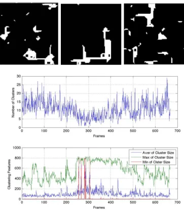
By treatingEas a cellular automata and observing its space- time diagrams when the network (E, I) is parametrized in such a way that it displays erratic spiking, we can observe what seem to be some meta-stable patterns. This is partic- ularly evident when we focus on the time step immediately before a spike. As one would assume, when(E, I)is spiking periodically the time step before a spike will periodically have the same active and inactive vertices. What is fascinating, and reaffirmed by Figure??, is that in the erratic spiking we see near repetitions for large spans of time and then a sudden shift into another type of near repetition. We demonstrate this in Figure 7. Since we are considering patterns in the time steps immediately preceding a spike and with relatively largem,E has almost all of its vertices active and it is more informative to consider the vertices which stay inactive in a step. We note that small clusters of inactivity seem to almost shift around, until they merge, become mostly repetitive, and then finally splinter back up. The top of Figure 7 shows snapshots of activity in E at these different patterns, the plot at the bottom of the figure shows us the biggest inactive cluster in a time step, the smallest in a time step, and the average.
Though we only show three snapshots, notice that in the bottom of Figure 7 the three plotted time series measuring inactivity cluster sizes are not behaving randomly. Using these
1To make the plots clear in this paper, we plotted (t, t0) when x(t)andx(t0)were both are within a ball whose radius we choose to contain minimally contains10points of the time series. This guarantees the plot is not extremely sparse since each time step has at least10points plotted against it. A careful introduction to recurrence plots can be found in [17], [18]
Fig. 4: Comparison of Poincar´e Section for m= 600,1180,1550,1860and embedding τ= 5; for m= 600,1180,and1550, the corresponding points are encircled for better visualization.
Fig. 5: Comparison of time-embedding delay of exponential decay activity time series for m = 600,1180,1550,1860 and embedding τ= 5.
(a) (b)
Fig. 6: Recurrence plot for parameter selections leading to various dynamics: (a) periodic oscillations (m= 1550; (b) absence of period within the observation interval (m = 1860). Notice the continuous (linear) curves in (a) and the presence of discontinuities in (b).
observations we can conclude that it is possible to tame the erratic spiking by controlling these meta-stable patterns. As such we re-ran the simulations of our network and introduced external stimuli in specific places for extended periods of time.
In Figure 8 we see a recurrence plot of a simulation initialized in exactly the same way as Figure 6b, but after 100000time steps we forced a connected component comprising of one fourth of the vertices in E into being active with a high probability for a total of 10000 time steps. Notice that near the origin of Figure 8 it is similar to Figure 6b, until suddenly we inject stimuli and it falls into a very structured regime and then returns to looking like Figure 6b when we stop injecting input.
We ran this experiment multiple times with similar results each time. The fact that erratic spiking quickly resumed itself after prolonged stimuli, over a large portion of the excitatory vertices each time is ample evidence that these dynamics are able to withstand accepting stimuli without being dominated by the perturbations. Furthermore, the temporary regularity in the face of the stimuli is precisely what we hope for in a model to be used for associative memories based on itinerant dynamics.
IV. CONCLUSIONS
We have introduced a lattice-based neural network with discrete time and space dynamics. This network consists of excitatory and inhibitory neurons and it is able to exhibit oscillatory dynamics. Various parametrizations influence the nature of the oscillators, producing phase transitions from fixed point, limit cycle, and non-periodic dynamics. We demon- strated that the inhibitory reset parameter can control the
oscillatory dynamics and that the oscillations are robust to input perturbations. These properties demonstrate the promise of our model to serve as the basis of associative memories, after incorporating a suitable learning rule. Our model has ad- vantages in digital computer implementations, as the discrete nature of the iterative dynamics makes it less susceptible to numerical errors while unfolding its dynamics.
Additional work is in progress along the following main directions: (i) formalizing the idea of activity/inactivity clus- ters so as to be able to do a proper mathematical analysis of the effects that stimuli have on the network; (ii) running simulations with more varied and irregular stimuli to see their effect on the network dynamics; (iii) expanding the experiments to large-scale networks; and (iv) implementing learning rules to use the network as dynamic associative memories. The results of these studies will be reported in a forthcoming publication.
V. ACKNOWLEDGMENTS
This work has been supported in part by Defense Advanced Research Project Agency Grant, DARPA/MTO HR0011-16- l-0006 and by National Science Foundation Grant NSF- CRCNS-DMS-13-11165. M.R. has been supported in part by NKFIH grant 116769.
REFERENCES
[1] A. Arieli, D. Shoham, R. Hildesheim, and A. Grinvald, “Coherent spatiotemporal patterns of ongoing activity revealed by real-time optical imaging coupled with single-unit recording in the cat visual cortex.”
Journal of Neurophysiology, vol. 75, May 1995.
[2] W. J. Freeman and Q. Quiroga,Imaging brain function with EEG and ECoG. Springer, 2012.
Fig. 7: Top: Snap shot at different times of the activity in E just before firing. Bottom: Time series of maximum sized, minimum sized, and the average size of clusters of inactivity during the time step just before firing. This shows us some meta-stable patterns in the erratic spiking of (E, I).
[3] W. Penny, K. Friston, J. Ashburner, S. Kiebel, and T. Nichols,Statistical Parametric Mapping. Academic Press, 2006.
[4] T. K. Berger, G. Silberberg, R. Perin, and H. Markram, “Brief bursts self- inhibit and correlate the pyramidal network,”PLoS Biology, September 2010.
[5] W. J. Freeman, “The physiology of perception,”Scientific American, vol.
264, February 1991.
[6] S. E. Boustani and A. Destexhe, “Does brain activity stem from high- dimensional chaotic dynamics? evidence from the human electroen- cephalogram, cat cerebral cortex and artificial neuronal networks.”
[7] R. Kozma and M. Puljic, “Hierarchical random cellular neural networks for system-level brain-like signal processing,”Neural Networks, vol. 45, pp. 101–110, September 2013.
[8] G. Palm, “Neural associative memories and sparse coding,” Neural Networks, vol. 37, 2013.
[9] J. J. Hopfield, “Neurons with graded response have collective compu- tational properties like those of two-state neurons,”Proceedings of the National Academy of Sciences, vol. 81, May 1984.
[10] T. Kenet, D. Bibitchkov, M. Tsodyks, A. Grinvald, and A. Arieli,
“Spontaneously emerging cortical representations of visual attributes,”
Nature, vol. 425, 2003.
[11] T. Sasaki, N. Matsuki, and Y. Ikegaya, “Metastability of active ca3 networks,”Journal of Neuroscience, vol. 27, 2007.
[12] A. Arieli, A. Sterkin, A. Grinvald, and A. Aertsen, “Dynamics of ongoing activity: explanation of the large variability in evoked cortical responses,”Science, vol. 273, 1996.
[13] T. Kurikawa and K. Kaneko, “Associative memory model with sponta- neous neural activity,”EPL, vol. 98, 2012.
[14] D.-W. Huang, R. Gentili, and J. Reggia, “Self-organizing maps based on limit cycle attractors,”Neural Networks, vol. 63, 2015.
[15] S. Janson, R. Kozma, M. Ruszink´o, and Y. Sokolov, “Bootstrap perco- lation on a random graph coupled with a lattice.”
Fig. 8: Recurrence plot showing the effect of input stimuli injected at a subset of nodes (in one corner of the lattice) for an extended period of time (10,000 time steps). The inputs cause the discontinuities seen in Fig. 6b to disappear, which means the non-periodic dynamics collapses to periodic oscillations;
(m= 1860).
[16] A. E. Holroyd, “Sharp metastability threshold for two-dimensional bootstrap percolation,”Probability Theory and Related Fields, 2003.
[17] J.-P. Eckmann, S. Kamphorst, and D. Ruelle, “Recurrence plots of dynamical systems,”Europhysics Letters, vol. 4, 1987.
[18] N. Marwan, M. C. Romano, M. Thiel, and J. Kurths, “Recurrence plots for the analysis of complex systems,”Physics Reports, vol. 438, 2007.