2.1. Study area

(1)

Analysing the vegetation of energy plants by processing UAV images ^*

Melinda Pap, Sándor Király, Sándor Molják

Eszterházy Károly University

(pap.melinda,kiraly.sandor,moljak.sandor)@uni-eszterhazy.hu Submitted: June 21, 2019

Accepted: January 4, 2020 Published online: January 9, 2020

Abstract

Bioenergy plants are widely used as a form of renewable energy. It is important to monitor the vegetation and accurately estimate the yield before harvest in order to maximize the profit and reduce the costs of production.

The automatic tracking of plant development by traditional methods is quite difficult and labor intensive. Nowadays, the application of Unmanned Aerial Vehicles (UAV) became more and more popular in precision agriculture. De- tailed, precise, three-dimensional (3D) representations of energy forestry are required as a prior condition for an accurate assessment of crop growth. Using a small UAV equipped with a multispectral camera, we collected imagery of 1051 pictures of a study area in Kompolt, Hungary, then the Pix4D software was used to create a 3D model of the forest canopy. Remotely sensed data was processed with the aid of Pix4Dmapper to create the orthophotos and the digital surface model. The calculated Normalized Difference Vegetation Index (NDVI) values were also calculated. The aim of this case study was to do the first step towards yield estimation, and segment the created orthophoto, based on tree species. This is required, since different type of trees have different characteristics, thus, their yield calculations may differ. How- ever, the trees in the study area are versatile, there are also hybrids of the same species present. This paper presents the results of several segmentation algorithms, such as those that the widely used eCognition provides and other Matlab implementations of segmentation algorithms.

Keywords:photogrammetry, 3D reconstruction, segmentation, NDVI.

*The research was supported by the grant EFOP-3.6.1-16-2016-00001 (“Complex improvement of research capacities and services at Eszterházy Károly University”).

doi: https://doi.org/10.33039/ami.2020.01.001 url: https://ami.uni-eszterhazy.hu

183

(2)

1. Introduction

Energy plants are important for preserving the Earth’s ecology and as alternative energy sources like bio-fuel. They play an important role both in producing biofuel and heating electricity-generating power stations. There are plenty of tree species (woody plants) that can be planted as energy plants, for example Gray Poplar (Populus canescens), White Poplar (Populus alba) or Red oak (Quercus rubra).

Precise and detailed three-dimensional (3D) representations of the forestry area are very important for an accurate assessment of their volume and growth. Un- til recently, measuring the volume, spatial arrangement and shape of trees with precision has been constrained by logistical and technological limitations and cost.

Traditional methods of plant biometrics provide merely partial measurements and these methods are labor intensive. Advances in Unmanned Aerial Vehicle (UAV) technology has made it feasible to obtain high-resolution imagery and three dimensional (3D) data using lightweight and inexpensive cameras. These are esential for energy plants monitoring and assessing tree attributes automatically [18].

In order to monitor and control the vegetation of plants and to measure their volume, it is necessary to create a 3D model from the UAV recorded 2D images.

For processing huge amounts of imaging data, there are two frequently applied approaches: structure-from-motion (SfM) and multi-view stereopsis (MVS). Both can operate without information on the 3D position of the camera or the 3D location of control points.

SfM is a cost-effective method for extracting the 3D model of a scene from multiple overlapping images using bundle adjustment procedures [17]. It can generate high quality 3D point clouds for characterizing forest structures and can be used to generate accurate Digital Surface Models (DSMs) from the 3D point clouds. The 3D representation of the surface of a terrain and DEM (Digital Elevation Model) is a subset, and the most fundamental component of DSM [4, 15, 21]. The DSM is essential in creating an orthophoto of the whole scanned area as a geometrically corrected uniform-scale photograph, it is possible to use it for measurements. The success of SfM is controlled by image resolution, the degree of image overlap, as well as the relative motion of the camera with respect to the scene [25]. Photos created by an UAV are ideal for SfM since UAV fly only a few tens of meters above the ground, providing data with high spatial resolution that is better than space- borne sensors. Therefore, UAVs have the potential of resolving the measurement of individual trees and plants for biomass estimation[24].

Image segmentation is the process of separating or grouping an image into different image objects. An image object is a group of connected pixels in a picture, where the objects are homogeneous with respect to specific features. These features can be represented by the RGB values, textures or gray-levels, each encoding similarities between the pixels of a region. Other segmentation methods focus on finding boundaries between regions. There are many different ways of performing image segmentation, ranging from the simple thresholding method to different colour image segmentation algorithms. In this paper, we aimed to find the best seg-

(3)

mentation algorithm for the purpose of segmenting an energy forest where hybrids of the same species are present. The goal is to find a method that is efficient but also robust in the sense that it is not strongly dependent on its input parameters.

Hossain and Chen [16] conducted an extensive state-of-the-art survey on OBIA (Segmentation for Object-Based Image Analysis) techniques, discussed different segmentation techniques and their applicability to OBIA. This article shows, that Ming et al. [12] implemented MeanShift algorithm for QuickBird ( high-resolution remote sensing imagery) and panchromatic images, Maurer [13] for cropland and Michel et al. [8] for multiple objects but none of them targeted energy plants. Li et al. [14] implemented SRM segmentation method for QuickBird imagery as well.

Csillik [3] proposed a segmentation workflow where MRS algorithm started from superpixels instead of individual pixels. He also used the quickBird dataset and reached accuracy above 90%. Instead of using a single scale for the entire image, Fonseca-Luengo et al. [6] offered a hierarchical multiscale segmentation using superpixels (SLIC) which allowed users to detect objects at different scales. They used a satellite image that was collected by the Pléiades Satellite, in the central irri- gated valley of Chile. Several researchers applied Region growing/merging, Region splitting and merging, Hybrid method (HM) and Semantic methods for different targets: road and agricultural land, fozen oil, sand ore, mixed vegetation, etc. but none for hybrid energy plants.

Tsouros et al. [23] reviewed the UAV-Based Applications for Precision Agricul- ture. This article shows that Zhao et al. [26] implemented segmentation method for targeting canopy pixels of pomegranate trees by using a fully convolutional neural network. Their tests on validation set showed that its precision reached above 90%

and it was robust to changes in camera settings, lighting condition, canopy development and changing background. They worked with LIDAR imagery. Hassain et al. [10] has introduced a new vegetation segmentation approach which aims to generate vegetation binary images from RGB images acquired by a lowcost UAV system. They reached 87.29% with standard deviation 12.5%, in the detection of any type of vegetation in an area. Their study did not involve distinguishing the types of vegetation. Parraga et al. [22] used an algorithm to segment wheat plots for two kinds of Brazilians wheat cultivates.

2. Methods

2.1. Study area

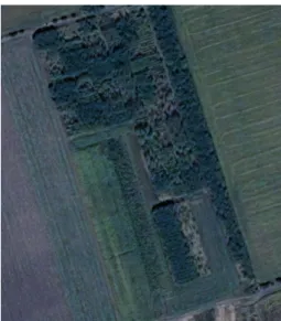
The study area is located in Kompolt, at the Rudolf Fleischman Research Institute of the Eszterhazy Karoly University (47.735889 N, 20.224807 W, see Fig. 1).

A variety of three species (willows, acacias, poplars) and six hybrids of poplar are present in this study area.

(4)

Figure 1: Satellite image of the study area from Google Earth

2.2. Data Acquisition and Processing

For this study, the aerial survey was conducted on 6 September 2018 using a DJI In- spire 2 quadcopter. Besides the built-in high-precision satellite positioning system, ultrasonic, infrared and optical sensors help the machine to navigate and operate autonomously. An IMU (Inertial Measurement Unit), compass and barometer also improved the navigation. The true colour sensor was a Zenmus X5S. Us- ing a 4/3inch CMOS sensor, the camera can produce images of a resolution of 20.8 megapixels. The camera was equipped with a 15 mm F/1.7 lens that has a FoV value of 72^∘. Multispectral images were taken with a Parrot Sequoia camera. The sensor has 4 multispectral sensors, capable of a resolution of 1.2 MP, and a 16 MP RGB sensor. In addition, the Sequoia has a sun sensor that eliminates changes in ambient light intensity. The camera and the sun sensor have also a built-in IMU and magnetometer, and the sun sensor also contains an integrated GPS. We applied the Altizure flight planning software to create multispectral sub- sides, since the application also supports individual cameras that are not directly connected to the drone. The Altizre was adapted to the unique viewing angle of the multispectral sensor, so the overlaps between the lines were accurate. The ground switch points were measured with a 216 channel GPS + Glonass signaling dual frequency Javad Triumph 2 GNSS rover. The GNSS receiver was controlled by a Carlson SurvPC installed on a Juniper Systems Mesa2 tablet computer. The RTK correction service was provided bywww.gnssnet.hu.

(5)

2.2.1. RGB images

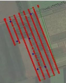
The flight altitude was 100 meters and the total flight time was 13 minutes 21 seconds. The overlap in the flight range was 90%, while the overlap between the two lines was 75%. The drone flew the hand-selected area of approximately326× 433meters at the set height and overlap in 7 flight lines. During the flight 263 images were taken in orthogonal camera positions. The georeference was specified with 7 ground connection points (see Fig. 2).

Figure 2: The flight path of the above study area and the Ground Control Points (GCPs)

2.2.2. Multispectral images

The multispectral investigation of the study area was performed at 70 meters and with a 70% overlap. The drone flew 8 flight lines at 6 m/s. The georeference was refined with 7 ground connection points. During the flight 788 images were taken from 197 positions and in 4 channels (Green, Red, Red edge, NIR) in an orthogonal camera position (see Fig. 3).

2.2.3. 3D reconstruction

The essence of 3D reconstruction is the assumption that the 3D point corresponding to a specific image point is constrained to the line of sight. Taking two images, we know that a 3D point that is present on both of the images is located at the intersection of the two projection rays. This process is also known as triangula-

(6)

Figure 3: The flight path above the study area and Ground Control Points (GCPs) – multispectral images

tion. Furthermore, we can conclude that corresponding sets of points must have a relationship that is related to the positions and the calibration of the camera.

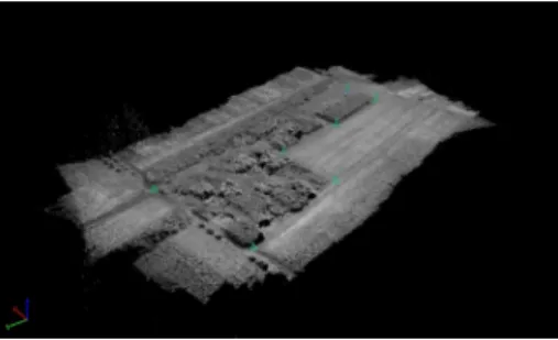
Figure 4: The 3D point cloud obtained from the RGB images

As a result of the photogrammetric processing, the average field resolution was 2.3 cm/pixel in the case of the RGB 3D model and the total processed area was 12.8 hectares. The number of the average key points was 72423. The average RMS error was 0.013 m. The finished 3D point cloud consists of over 34 million points (Figure 4), averaging 2614 points 𝑚². After the photogrammetric processing of the images taken by multispectral camera the average field resolution was 7.7 cm/pixel, the total processed area was 12.3 hectares. The average RMS error was 0.023 m. The finished 3D point cloud consists of over 412,000 points, averaging

(7)

2.21 points/𝑚² (see Figure 5).

Figure 5: The 3D point cloud obtained from the multispectral images

Using Pix4Dmapper photogrammetry software, the digital surface model was created in the WGS 1984 UTM Zone 34N coordinate system. The achieved spatial resolution was 2 cm/pixel at an average height of 95.5 meters. The difference between the lowest and the highest point is 21.5 meters (see Figure 4). Applying the Pix4Dmapper software, we also created the NDVI map of the study area in the WGS 1984 UTM Zone 34N coordinate system. The spatial resolution of the map is 6.9 cm/pixel and the average NDVI is 0.78. The lowest value was 0.28 and the highest one was 0.95 (see Figure 6a).

2.2.4. Segmentation Methods

The difficulty of the segmentation of species arises from the presence of hybrids.

They have similar characteristics in height and colour; therefore they are barely distinguishable even to the human eye. There are a vast amount of segmentation methods already in the literature. We aimed at selecting the ones that are based on colour rather than edges or shapes present in images. We used the most widespread segmentation methods in the field of agriculture such as Multiresolution segmentation provided by the eCognition software and the Mean shift segmentation implemented in Matlab. In addition to these algorithms we also investigated the usability of the Statistical Region Merging method.

2.2.5. Multiresolution segmentation (MRS)

We investigated the eCognition’s hierarchical, multiresolution (MRS) algorithm.

This algorithm combines pixels or objects, so it is based on region growing. Also this is an optimization method that minimizes the average heterogeneity with a given number of objects and maximizes the homogeneity of the object. It merges objects that best fit each other. The steps of the algorithm:

∙ Step 1: each pixel is an independent object. These are combined in several steps into larger objects until they reach a certain homogeneity threshold.

(8)

This threshold is derived from spectral and formal homogeneity values that can be specified in the parameter.

∙ Step 2: Find the best matched neighbor for each core object that is created in the first step.

∙ Step 3: If the best fit is not mutual, the object in the comparison will be the next object tested.

∙ Step 4: If the best fit is mutual, the two objects are merged.

∙ Step 5: In each iteration, each object is tested once.

∙ Step 6: Iteration stops if there is no additional merge option.

The following parameters can be set:

∙ Layer weights: selection and weighting of the layers we want to apply during segmentation. It increases the weighting of the layer when calculating the heterogeneity measure used to decide whether pixels/objects are merged.

Zero ignores the layer.

∙ Scale parameter(r): maximum allowed heterogeneity within an object. It controls the amount of spectral variation within objects and therefore their resultant size. It can be any positive, integer number.

∙ Shape(s): the degree of spectral and geometric homogeneity (colour = 1 - shape). A weighting between the objects shape and its spectral colour whereby if 0, only the colour is considered whereas if > 0, the objects shape along with the colour are considered and therefore less fractal boundaries are produced. The higher the value, the more that shape is considered.

∙ Compactness(c): compactness of objects. A weighting for representing the compactness of the objects formed during the segmentation [1]. It can be a value between 0 and 1.

By changing these parameters and the input layers the size and shape of image objects are almost endlessly modifiable. The ability to perform other types of segmentation such as conditional or classification-based segmentation makes limitless modifications to the results of multiresolution segmentation possible. Sadly, it is a semiautomatic approach, there is no generally applicable formula for assigning layer weights, setting the parameters, and implementing segmentation - ultimately, trial and error and experience are the best guides [9].

2.2.6. Statistical Region Merging (SRM)

The Statistical Region Merging (SRM) Segmentation algorithm proposed by the authors of [20] is a time efficient method that operates as follows. It defines a real-valued function of similarity 𝑓(𝑝0;𝑝1), where the 𝑝0 and 𝑝1 are two different

(9)

points in the image. It takes each pair of points and sorts the pairs based on their similarity. In the next step, it iterates through the sorted pairs that are not yet in the same region and merges their two regions if a predefined probabilistic function returns true. The value of the function 𝑓 is based on the between-pixel local gradients, and their maximal perchannel variation.

The algorithm takes one argument, the scale parameter𝑄that defines the sizes of expected regions relative to the size of the original image. By choosing the value of 𝑄for smaller results in larger segments, while choosing it for greater results in small segments.

2.2.7. Mean shift

The Mean Shift Segmentation (MSS), proposed in [7], is based on the assumption that the feature space is a probabilistic density function. The dense regions in the feature space correspond to local maximas. So for each data point, the algorithm performs a gradient ascent on the local estimated density until convergence. The stationary points obtained through gradient ascent represent the local maximas of the density function. All points associated with the same stationary point belong to the same cluster. The MSS only requires one parameter: the spatial radius𝑟𝑠.

3. Results and discussion

3.1. NDVI and DEM

The created maps (NDVI and DEM) are suitable to track the vegetation of plants.

The NDVI (Normalized Difference Vegetation Index) was developed to give an insight of plant presence and health. It is calculated as follows:

NDVI=𝑎_nir−𝑎_vis 𝑎nir+𝑎vis,

where 𝑎nir is the surface reflectance in the near infrared channel, and 𝑎vis is the reflectance in the visible red channel [2]. The NDVI map indicates where an area has healthy vegetation (green areas) and also the segments where the vegetation is low, i.e. the NDVI values are below 0.6 (yellow and red areas). With the incorpo- ration of the DEM it is possible to locate areas where the canopy is low, as well as detect the lack of trees. As it is visible in Figure 6, compared to the NDVI map it can be seen that the hight of the plants correlates with low vegetation.

3.2. Preprocessing methods

When analyzing the orthophotos, it was found that the leaves of the same species did not have the same intensity value. Furthermore, the canopy of trees always have small gaps between leaves, branches and crowns. To eliminate the differences, two types of blur filters were used: Gauss filter and Median filter. The latter is a

(10)

(a) NDVI map (b) DEM map Figure 6: The calculated NDVI and DEM images

nonlinear filter being used frequently to remove the “salt and pepper” image noise while preserving edges. The effect of Gaussian smoothing is also to blur the image.

The degree of smoothing is determined by the standard deviation of the Gaussian and it outputs a “weighted average” of each pixel’s neighborhood. Both methods were used with versatile kernels.

3.3. Evaluation method

We evaluated the results of the segmentation methods by an external cluster valid- ity index, the Sorensen-Dice similarity coefficient (𝐷) [5]. Based on the conclusions stated in [19], the𝐷is a suitable measure for evaluation in the field of biogeography since it is less sensitive to outliers than the other coefficients. The coefficient 𝐷 is calculated as follows:

𝐷= 2𝑎

2𝑎+𝑏+𝑐,

where 𝑎 is the number of point pairs that belong to the same segment in the ground truth as well as in the segmentation result,𝑏 is the number of point pairs that belong to the same segment in the ground truth, but to different ones in the segmentation result and𝑐is the number of point pairs that are in different segments in the ground truth, but in the same segment in the segmentation result.

3.4. Segmentation

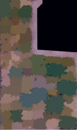
We used the aforementioned segmentation algorithms: MRS, SRM and MSS. In order to evaluate the results of segmentations, we first had to create the ground

(11)

truth image for the area. This images is presented in Figure 7b.

The goal was to find a method that is efficient but also robust in the sense that it is not strongly dependent on its input parameters. First we evaluated the eCognition’s MRS segmentation algorithm that is the state of the art currently in this field of application. This is a semi-automatic process, it requires the users supervision to achieve the best results. Therefore, to reach the accuracy of this method was the goal for the other, unsupervised methods. The different segmentation methods were used with varying preprocessing methods. The segmentation methods also differ in their inputs.

(a) The original orthophoto (b) The ground truth image Figure 7: The original orthophoto and the corresponding ground

truth image

In the MRS of eCognition, the user can select the RGB channels and can add the DEM and the NDVI of the original image as a new layer. The above mentioned parameters were selected empirically in our study. The image layer weights were set for RGB channels (1,5,10 and 1,10,5), for DEM (between 1 and 10) and for NDVI (between 1 and 10). The scale parameter was tested between 100 and 240.

Our shape parameter was set between 0.01 and 0.4, the compactness parameter was between 0.6 and 1.0. For the original size images, the application of filters resulted in worse results. For the resampled (reduced to 75%) images, we got slightly worse results (68–71% accuracy) and the applied filters also resulted in weaker results.

(12)

Reducing the size of the original orthophoto (and both DEM and NDVI images) to 50% led to results below 50%. The best results were obtained by performing this algorithm on the image reduced to one quarter of the original size with the layers: 1,5,10 of the RGB channels respectively, 2 for the DEM layer and 0 to the NDVI layer, the other parameters were set as follows: 𝑟= 240, 𝑠 = 0.4, 𝑐= 0.9.

After the first run of the algorithm, further hierarchical segmentation was applied by selecting regions that we wished to further split and the segmentation method was rerun on that region only. After performing such steps repeatedly, we reached the highest accuracy: 73.15% (Fig. 8).

Figure 8: The segmented objects after performing multiresolution segmentation for the study area

The Matlab implementation of the MSS only required one parameter: the spatial radius 𝑟𝑠. The rest of the settings of the algorithm are calculated from this parameter. The parameter𝑟𝑠was tested with the values0.05,0.06, . . . ,0.1.

For preprocessing, the Median filter was tested with two kernel sizes: 9 and 12. The used kernel sizes of the Gauss filter were 2 and 3, the application of preprocessing methods improves the segmentation accuracy significantly regardless of the type of smoothing operator. The best accuracy, 80.70% was reached on the

(13)

RGB image resampled to 10% of the original size and filtered by a Gauss filter of kernel size 3 and the rs set to 0.07.

We have used the Matlab implementation of the SRM algorithm provided by the authors of [20]. We tested this algorithm with the RGB images downsampled to 10% of the original size. The Median and Gauss smoothing filters were also tested as preprocessing steps before the application of the SRM. The values for the scale parameter𝑄were selected from the range [100,3000] on a logarithmic basis as it was proposed by the authors of [20]. The Median filter was tested with two kernel sizes: 9 and 12. The used kernel sizes of the Gauss filter were 2 and 3. The achieved best accuracy was 62.45%.

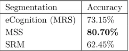
The summary of the best accuracies of the used segmentation methods is shown in Table 1.

Segmentation Accuracy eCognition (MRS) 73.15%

MSS 80.70%

SRM 62.45%

Table 1: Results of segmentations

4. Conclusions

One aim of this case study was to investigate the applicability of a lowcost UAV in the field of precision agriculture. On other goal was to find a suitable segmentation method that is able to operate on an image that contains several hybrids of the same tree species, a task which is hard even for the human eye. Many studies were solving segmentation problems on areal imagery, however, these mostly aimed at detecting vegetation and distinguishing it from the surrounding landmarks [6, 8, 10, 12]. Our goal was to perform the task of segmenting tree species apart, that is an even more challenging task with hybrids present.

The created precise 3D model is suitable for agriculture experts to examine energy plantation, the NDVI and DEM maps can be used to observe vegetation in the study area and to give a mass estimate. The orthophoto obtained from the 3D model can be used for segmentation. The eCognition’s MRS reached 73.15%

accuracy when the DEM was added to the RGB orthophoto as a layer. With the help of the NDVI map added to the RGB image as a layer we got worse segmentation results. The Matlab implementation of the MSS algorithm was the parameter insensitive method that reached the highest accuracy with 80.70%.

(14)

References

[1] J. van Aardt,R. Wynne:A Multiresolution Approach to Forest Segmentation as a Pre- cursor to Estimation of Volume and Biomass by Species, in: Jan. 2004.

[2] A. Bannari,D. Morin,F. Bonn,A. R. Huete:A review of vegetation indices, Remote Sensing Reviews 13.1-2 (1995), pp. 95–120,

doi:https://doi.org/0.1080/02757259509532298.

[3] O. Csillik:Fast segmentation and classification of very high resolution remote sensing data using, Remote Sens 9.3 (2016), p. 243,

doi:https://doi.org/10.3390/rs9030243.

[4] A. Cunliffe,Brazier:Ultrafine grain landscape-scale quantification of dryland vegetation structure with drone-acquired structure-from-motion photogrammetry, Remote Sensing of Environment 183.1 (2016), pp. 129–143,

doi:https://doi.org/10.1016/j.rse.2016.05.019.

[5] L. R. Dice:Measures of the amount of ecologic association between species, Ecology 26.3 (1945), pp. 297–302.

[6] D. Fonseca-Luengo,A. García-Pedrero,M. Lillo-Saavedra, et al.:Optimal scale in a hierarchical segmentation method for satellite images, in: International Conference on Rough Sets and Intelligent Systems Paradigms, New York, NY, USA: Springer, Cham, 2014, pp. 351–358,

doi:https://doi.org/10.1007/978-3-319-08729-0_36.

[7] K. Fukunaga,L. Hostetler:The estimation of the gradient of a density function, with applications in pattern recognition, in: IEEE Transactions on information theory, New York, NY, USA: IEEE, 1975, pp. 32–40,

doi:https://doi.org/10.1109/TIT.1975.1055330.

[8] M. Grizonnet,J. Michel,V. Poughon, et al.:Orfeo ToolBox: open source processing of remote sensing images, Open geospatial data, softw. stand 2 (2017), Article number: 15, doi:https://doi.org/10.1186/s40965-017-0031-6.

[9] R. Hamilton,K. Megown,T. Mellin,I. Fox:Guide to automated stand delineation using image segmentation, Oct. 2007.

[10] M. Hassanein,N. El-Sheimy:An efficient weed detection procedure using low-cost UAV imagery system for precision agriculture applications, in: Int. Arch. Photogramm. Remote Sens. Spatial Inf. Sci. Karsluhe, Germany: ISPRS rs, 2018, pp. 181–187,

doi:https://doi.org/10.5194/isprs-archives-XLII-1-181-2018.

[11] G. J. Haya,T. Blaschkeb,D. J. Marceaua,A. Bouchard:A comparison of three image-object methods for the multiscale analysis of landscape structure, ISPRS Journal of Photogrammetry and Remote Sensing 57.5-6 (2003), pp. 327–345,

doi:https://doi.org/10.1016/S0924-2716(02)00162-4.

[12] M. Hossain,D. Chen:Segmentation for Object-Based Image Analysis (OBIA): A review of algorithms and challenges from remote sensing perspective, ISPRS Journal of Photogram- metry and Remote Sensing 150.6 (2019), pp. 115–134,

doi:https://doi.org/10.1016/j.isprsjprs.2019.02.009.

[13] J. W. Karl,B. A. Maurer:Spatial dependence of predictions from image segmentation:

A variogram-based method to determine appropriate scales for producing landmanagement information, Ecological Informatics 5 (2010), pp. 194–202,

doi:https://doi.org/10.1016/j.ecoinf.2010.02.004.

[14] H. Li,H. Gu,Y. Han,J. Yang:An efficient multiscale SRMMHR (Statistical Region Merging and Minimum Heterogeneity Rule) segmentation method for high-resolution remote sensing imagery, Open geospatial data, softw. stand 2.2 (2009), pp. 67–73,

doi:https://doi.org/10.1109/JSTARS.2009.2022047.

(15)

[15] S. Messinger,Asner:Rapid assessments of Amazon forest structure and biomass using small unmanned aerial systems, Forests 8.8 (2016), p. 615,

doi:https://doi.org/10.3390/rs8080615.

[16] D. Ming,J. Li,J. Wang,M. Zhang:Scale parameter selection by spatial statistics for GeOBIA:Using mean-shift based multi-scale segmentation as an example, ISPRS Journal of Photogrammetry and Remote Sensing 106 (2015), pp. 28–41,

doi:https://doi.org/10.1016/j.isprsjprs.2015.04.010.

[17] R. Mlambo,I. H. Woodhouse,F. Gerard,K. Anderson:Structure from motion (sfm) photogrammetry with drone data: a low cost method for monitoring greenhouse gas emissions from forests in developing countries, Forests 8.3 (2017), p. 68,

doi:https://doi.org/10.3390/f8030068.

[18] M. Mohan,C. A. Silva,C. Klauberg, et al.:Individual tree detection from unmanned aerial vehicle (uav) derived canopy height model in an open canopy mixed conifer forest, Forests 8.9 (2017), p. 340,

doi:https://doi.org/10.3390/f8090340.

[19] M. Murguía,J. L. Villaseñor:Estimating the effect of the similarity coefficient and the cluster algorithm on biogeographic classifications, Annales Botanici Fennici. JSTOR 40.6 (2003), pp. 415–421.

[20] R. Nock,F. Nielsen:Statistical region merging, in: IEEE Transactions on pattern analysis and machine intelligence, New York, NY, USA: IEEE, 2004, pp. 1452–1458,

doi:https://doi.org/10.1109/TPAMI.2004.110.

[21] B. St-Onge,J. Jumelet,M. Cobello,C. Véga:Measuring individual tree height using a combination of stereophotogrammetry and lidar, Canadian Journal of Forest Research 34.1 (2004), pp. 2122–2130,

doi:https://doi.org/10.1139/x04-093.

[22] A. Parraga,D. Doering,J. G. Atkinson, et al.:Wheat Plots Segmentation for Exper- imental Agricultural Field from Visible and Multispectral UAV Imaging, in: SAI Intelligent Systems Conference, London, UK: Springer Cham, 2018, pp. 388–399,

doi:https://doi.org/10.1007/978-3-030-01054-6_28.

[23] D. C. Tsouros,S. Bibi,P. G. Sarigiannidis:A Review on UAV-Based Applications for Precision Agriculture, MDPI 10.11 (2019), p. 349,

doi:https://doi.org/10.3390/info10110349.

[24] H. Watts,Ambrosia:Unmanned aircraft systems in remote sensing and scientific research:

Classification and considerations of use, Forests 4 (2012), pp. 1671–1692, doi:https://doi.org/10.3390/rs4061671.

[25] G. H. Westoby,Brasington,Reynolds:Structure-from-motion photogrammetry: A lowcost, effective tool for geoscience applications, Geomorphology 4.6 (2012), pp. 300–314, doi:https://doi.org/10.1016/j.geomorph.2012.08.021.

[26] T. ZHao,H. Niu,E. de la Rosa, et al.:Tree canopy differentiation using instance-aware semantic segmentation, in: Proceedings of the 2018 ASABE Annual International Meeting, NSt. Joseph, MI, USA: American Society of Agricultural and Biological Engineers, 2018, p. 1.