COMPARISON OF FORECASTING METHODS FOR FREIGHT TRANSPORTATION BY POLISH RAILWAYS

DOI: 10.1556/606.2019.14.2.5 Vol. 14, No. 2, pp. 51–60 (2019) www.akademiai.com

COMPARISON OF FORECASTING METHODS FOR FREIGHT TRANSPORTATION BY POLISH

RAILWAYS

Wojciech KAMIŃSKI^*

Department of Logistics and Transport Technologies, Faculty of Transport Silesian University of Technology, Krasińskiego 8, 40-019 Katowice, Poland

e-mail: Wojciech.Kaminski@polsl.pl

Received 11 December 2018; accepted 9 March 2019

Abstract: In Poland problem related to lack of rolling stock occurred recently. This article presents a comparison between two forecasting methods of realized transport work and transported freight mass by railway. The obtained results are also compared on a monthly and quarterly data basis. Knowing the exact values of forecasts railway carriers can plan the number of rolling stock. The calculations show that using the data as a monthly basis, the most reliable results can be obtained using the Holt model, while calculating data for quarterly basis results is closer to the real values using the Winters model.

Keywords: Railway transport, Freight transport, Forecasting, Holt model, Winters model

1. Introduction

Currently on the railway freight transport in Poland the problems are related to lack of rolling stock (both locomotives and wagons). It is connected with long-term negligence consisting of the discontinuation repairing of subsequent series of locomotives, many wagons and insufficient quantity of new rolling stock purchased.

The main carrier on the rail freight transport is Polish National Railways (PNR) in Poland. Cargo, whose share in the transported freight mass in 2017 amounted to 44.5%, whereas in the realized transported work it is 51.9%, efficiently transport loads on electrified lines, while it is struggling with serious shortages of diesel locomotives, necessary for pulling heavy trains with coal or handling aggregate ramps. Similarly, the

* Corresponding Author

shortages of the rolling stock appear in the case of wagons. For several years, the volume of transported freight mass by railway in Poland has been increasing, which causes growth in the demand for rolling stock. In the first half of 2018, the PNR Cargo Company added to the traffic an additional 3 thousand wagons were waiting so far for revisions. It was associated with increased transport of aggregates (by 35% compared to the first half of 2017) and coal (by 3.1% compared to the same period previous year).

All rolling stock resources were used to carry out the ordered transports [1]. The high demand for wagons is also related to the low permissible speed on some railway lines.

Speed limits are often caused by improper railway tracks geometry resulting from the destruction [2]. Another problem is the numerous speed limits associated with the poor technical condition of railway bridges [3]. More rolling stock is necessary for the realization of increased freight transport. In order to avoid the problem related to the lack of rolling stock a forecast of the transported freight mass and the realized transport work using the current transport data should be made. Forecasts will allow determining approximate transport volumes in near future. The obtained transport volumes will be necessary to prepare rolling stock needed for increasing freight mass. Using data from forecasts gives time to repair locomotives and wagons or to purchase new ones. Most transport decisions should be made under conditions of data uncertainty and uncertainty of measurements, because some data and some limitations are difficult to measure [4].

The purpose of this article is to compare statistical methods of forecasting, which will allow the selection of the most appropriate method allowing for preparation forecast of realized transport work and transported freight mass by rail. For this purpose, forecasts will be prepared using two different methods. The used data covers the period from January 2010 to June 2018. In order to compare the impact of the data type on the received values, data will be used both on monthly and quarterly basis. The forecast will be carried out for the period from July 2018 until December 2020.

2. Forecasting

Forecasting is the process of predicting future events by analyzing the phenomena that currently occur. This is a complex issue, whose aim is to reduce risk during making decisions. Those who prepare forecasts during their work must overcome certain difficulties, for example by obtaining relevant statistical data, their verification and selection of the appropriate method of forecasting [5]. Making forecasts presents many challenges for the person performing them and is characterized by a high level of uncertainty. For a particular type of data, it is important to choose a forecasting method to take into account the relevant factors [6]. Forecasts give the best results with easy to measure and obtained data [7]. Forecasting models allow better insight into the changes in transport volumes [8]. Having data from the past, which were observed and recorded for statistical purposes, statistical methods are used to make predictions, because they are independent of expert assessments. Causal analysis methods are opposite to the statistical methods, which are used when it is not possible to distinguish the development trend of the predicted variable or when it is not possible to obtain reliable statistical data [9]. Forecasting by the use of expert opinions is also applied in rapidly changing situations when time series represent turning points or when there are some

structural changes in the analyzed time series [10]. Expert’s opinion is based on his experience and intuition. Assessing experts have profound knowledge of the problem being analyzed [11]. Another way to make predictions is a hybrid approach that combines statistical and expert forecasting methods. Statistical prediction is based on accurate data. By introducing an additional approach based on experts’ opinions, it makes it possible to increase the accuracy of the forecasts made [12]. In order to estimate the quantity of transported goods, the majority of people making forecasts use four-stage models, which take into account the generation of travel needs, distribution, choice of means of transport and choice of the route [13]. Determining the estimated transport volume would not be possible without correctly made forecasts based on transport volumes from previous periods [14]. Performing an accurate forecast requires the use of complex forecasting tools. However, it is enough to use simple models, for example the Holt or Winters model, to perform the initial forecast [15]. An important issue when forecasting should be the question what requirements must be met by the results obtained. After completing the calculations, it is possible to assess whether the obtained results meet the assumed goal [16]. Forecasts in this article will be made on the basis of current transport data. Factors like modernization of railway lines (building the second track, electrification of the line) will be omitted [17]. This is related to the fact that currently electrification lines of high importance in freight traffic are not planned. Electrified sections, for example Stalowa Wola - Lublin or Węgliniec - Zgorzelec, have marginal importance for freight traffic.

3. Data used for analysis

The source data of realized transport work and the transported freight mass by all rail carriers in Poland are reported by the Office of Rail Transport. According to the transported freight mass in the period from January to June 2018, the largest carrier in Poland is PNR Cargo, which transported 43.07% of the total cargo mass. The second very big carrier is German Railways (GR) Cargo Poland with a result of 16.99% of the transported freight mass. Other significant rail carriers are: Lotos Railway with 4.97%

of the transported freight mass, PNR Broad-gauge Ironworks Line (BIL) with 4.47% of mass, Chem Trans Logistic (CTL) 4.31% of mass, Railway Service Company (RSC) Kolprem with 3.12% of mass, Freightliner Poland with 2.41% of mass and Orlen Kol- Trans with 2.07% of the transported freight mass. In total, according to the license issued by the President of the Office of Rail Transport, in 2018 there are 65 carriers operating in Poland involved in the freight transport. At present, the rail freight transport market in Poland is showing an upward trend. In the period from January to June 2018 7.66% more freight mass was transported than in the corresponding period in 2017. A similar trend can be seen in the realized transport work, which increased by 12.08% in comparison to the previous year [18].

3.1. Realized transport work

The value of the realized transport work was presented in millions of tons- kilometers. For the purpose of a detailed analysis of this data series, statistical measures

for monthly data were calculated using statistical calculation software PQStat. The average value of realized transport work is 4271.8 million tkm. The median value is 4346.2 million tkm, so half of the monthly transport data takes levels lower than this value and half the higher. The minimum value of realized transport work occurred in January 2010 and amounted to 2972.3 million tkm. The maximum value of realized transport work occurred in March 2018 and amounted to 5029.54 million tkm. The range, therefore the difference between the maximum and minimum value of the realized transport work, is 2057.2 million tkm. The lower quintile dividing the data in the series by 25% and 75% is 4061.1 million tkm, while the upper quintile dividing the data into 75% and 25% is 4617.3 million tkm. The standard deviation, informing how widely individual values are separated from the average value, is 437.0 million tkm. The coefficient of variation for realized transport work is 10.2%.

3.2. Transported freight mass

The value of the transported freight mass was presented in millions of tons. For detailed analysis of this data series, statistical measures were calculated using statistical calculation software PQStat. The average value of transported freight mass is 19.4 million tons. The median is 19.6 million tons. The minimum value of transported freight mass was in February 2015 and amounted to 15.3 million tons. The maximum value of transported freight mass occurred in October 2010 and amounted to 22.6 million tons.

The range is 7.3 million tons. The lower quintile is 18.7 million tons, while the upper quintile is 20.7 million tons. The standard deviation is 1.6 million tons. The coefficient of variation for transported freight mass is 8.4%.

4. Models used to make forecasts

Forecasting was realized using Holt exponential smoothing model and Winters model, which take into account seasonal fluctuations. It made it possible to compare the results obtained with these methods [19].

4.1. Holt model

The Holt model is a two-equation model, which belongs to the group of exponential smoothing models. The predicted value is described in it using the first degree polynomial [19]. The equations of the model are shown below:

(

) (

)

+

= _{t t t}

t y F S

F α α , (1)

(

)

(

)

= _{t t t}

t F F S

S β β , (2)

where α,β∈<0;1>; Ft is the smoothed trend value of the forecasted variable for a period (t–1); St is the smoothed trend value increment forecasted for a period (t–1).

Expired forecasts in the Holt model are calculated using the formula:

t t

t F S

y)₊₁= + ₍₃₎

4.2. Winters model

The Winters model belongs to the group of exponential smoothing models, it is used when the time series of the predicted variable has a development tendency and seasonal fluctuations. The forecast is calculated using three equations containing three different smoothing parameters [19]. The equations of the model are shown below:

(

) (

)(

)

= _{t t r t t}

t y C F S

F α α , (4)

(

) (

)

= _{t t t}

t F F S

S β β , (5)

(

) ( )

t y F C

C =γ − + 1−γ ₋ , (6)

where α,β,γ∈<0 ;1>; Ft is the smoothed trend value of the forecasted variable for a period (t–1); St is the smoothed trend value increment forecasted for a period (t–1); Ct is the assessment of the seasonality index; r is the number of phases in the repeated cycle and n is the length of the time series.

Expired forecasts in the Winters model are calculated using the formula:

r t t t

t F S C

y)₊₁= + + _{+1− (7)}

5. The analysis of the received results of forecasts

In order to compare the usefulness of the Holt and Winters model to the creation forecasts of realized transport work and transported freight mass by rail were compared to the errors of expired forecasts. In addition, the obtained results were compared for monthly and quarterly data basis to assess the impact of the data type on the results of forecasts.

5.1. Forecasts of realized transport work and transported freight mass for monthly data basic

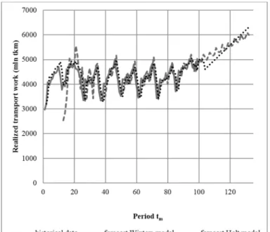
Monthly data were used in the period from January 2010 (tm=1) until June 2018 (tm=102). The forecast was made for the period from July 2018 (tm=103) to December 2020 (tm=132). The obtained results for realized transport work are presented in Fig. 1, and for transported freight mass in Fig. 2.

5.2. Forecasts of realized transport work and transported freight mass for quarterly data basis

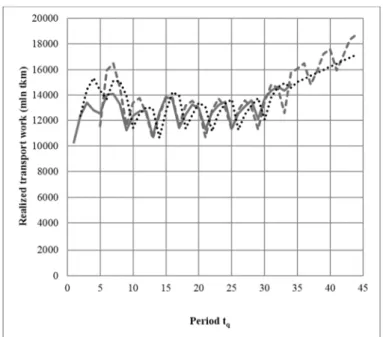
Quarterly data were used in the period from the first quarter 2010 (tq=1) to the second quarter 2018 (tq=34). The forecast was made for the period of the third quarter

2018 (tq=35) to the fourth quarter 2020 (tq=44). The obtained results for realized transport work are presented in Fig. 3, and for transported freight mass in Fig. 4.

Fig. 1. Forecasts of realized transport work for monthly data

Fig. 2. Forecasts of transported freight mass for monthly data

Fig. 3. Forecasts of realized transport work for quarterly data

Fig. 4. Forecasts of transported freight mass for quarterly data

5.3. Comparison errors of expired forecasts

Comparison errors of expired forecasts of realized transport work are presented in the Table I.

Table I

Comparison errors of expired forecasts realized transport work Data basis: Forecasting method: The average value

of relative forecast errors:

Square root of the average forecast error: (in millions)

monthly Holt model 6.31% 338.58 tkm

monthly Winters model 6.85% 406.52 tkm

quarterly Holt model 9.27% 1389.08 tkm

quarterly Winters model 4.39% 820.78 tkm

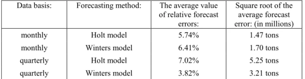
Comparison errors of expired forecasts transported freight mass are presented in Table II.

Table II

Comparison errors of expired forecasts transported freight mass Data basis: Forecasting method: The average value

of relative forecast errors:

Square root of the average forecast error: (in millions)

monthly Holt model 5.74% 1.47 tons

monthly Winters model 6.41% 1.70 tons

quarterly Holt model 7.02% 5.25 tons

quarterly Winters model 3.82% 3.21 tons

6. Conclusions

Based on the calculations made, it can be stated that for both realized transport work and transported freight mass by rail transport in Poland using the data as a monthly basis expired forecast results are closer to the real values using the Holt model, where the average value of relative forecast errors is 6.31%, and the square root of the average forecast error is 338.58 million tkm.

However, when calculating the data for quarterly basis, the most reliable results can be obtained using the Winters model, for which the average value of relative forecast errors is 4.39%, and the square root of the average forecast error is 820.78 million tkm.

To calculate the estimated volume of transport allowing for rolling stock preparation, quarterly data will be sufficient and used in one of the analyzed methods.

The use of quarterly data basis instead of monthly data basis allows receiving smaller error values. In the case of forecasting using quarterly data, better results are obtained

using the Winters model; however the error differences in both methods are small, so to obtain the estimated results is needed to enable the use of the somewhat simplistic Holt model.

References

[1] Szymajda M., PNR Cargo: We use all our rolling stock, we have good results (in Polish), Rynek Kolejowy Co, https://www.rynek-kolejowy.pl/wiadomosci/pkp-cargo- wykorzystujemy-wszystkie-nasze-zasoby-taborowe-mamy-niezle-wyniki-88336.html, (last visited 20 September 2018).

[2] Nagy R. Description of rail track geometry deterioration process in Hungarian rail lines No.1 and No.140, Pollack Periodica, Vol. 12, No. 3, 2017, pp. 141‒156.

[3] Major Z. Special problems of interaction between railway track and bridge, Pollack Periodica, Vol. 8, No. 2, 2013, pp. 97‒106.

[4] Moretti F., Pizzuti S., Panzieri S, Annunziato M. Urban traffic flow forecasting through statistical and neural network bagging ensemble hybrid modeling, Neurocomputing, Vol. 167, 2015, pp. 3‒7.

[5] Chudy-Laskowska K., Wierzbińska M. Chudy-Laskowska K., Wierzbińska M., Short-term forecast of the number of passengers transported by road in Poland (in Polish), Vntu, Vol.

25, No 65, 2012, pp. 330‒334.

[6] Kolosz B. W., Grant-Muller S. M. A macroscopic forecasting framework for estimating socioeconomic and environmental performance of intelligent transport highways, IEEE Transactions on Intelligent Transportation Systems, Vol. 15, No. 2, 2014, pp. 723‒736.

[7] Nuzzolo A., Comi A. Urban freight demand forecasting: A mixed quantity/delivery/

vehicle-based model, Transportation Research, Part E: Logistic and Transportation Review, Vol. 65, 2014, pp. 84‒98.

[8] Mackenbach J. D., Randal E., Zhao P., Howden-Chapman P. The influence of urban land- use and public transport facilities on active commuting in Wellington, New Zealand: Active transport forecasting using the WILUTE model, Sustainability, Vol. 8, No. 3, 2016, pp. 242‒256.

[9] Cisowski T., Stokłosa J. Traffic prognosis in transportation region, (in Polish) Technika Transportu Szynowego, Vol. 21, No. 9, 2014, pp. 36‒38.

[10] Scarpel R. A. Forecasting air passengers at Sao Paulo international airport using a mixture of local experts’ model, Journal of Air Transport Management, No. 26, 2013, pp. 35‒39.

[11] Xie G., Wang S., Lai K. K. Short-term forecasting of air passenger by using hybrid seasonal decomposition and least squares support vector regression approaches, Journal of Air Transport Management, Vol. 37, 2014, pp. 20‒26.

[12] Xie Z., Jia L., Qin Y., Wang L. A hybrid temporal-spatio forecasting approach for passenger flow status in Chinese high-speed railway transport hub, Discrete Dynamics in Nature and Society, Vol. 2013, Paper No. 239039, 2013, pages 7.

[13] Gutierrez J., Cardozo O. D., Garcia-Palomares J. C. Transit ridership forecasting at station level: an approach based on distance-decay weighted regression, Journal of Transport Geography, Vol. 19, No. 6, 2011, pp. 1081‒1092.

[14] Mrówczyńska B., Łachacz K., Haniszewski T., Sładkowski A. A comparison of forecasting the results of road transportation needs, Transport, Vol. 27, No. 1, 2012, pp. 73‒78.

[15] Mrówczyńska B., Cieśla M, Król A., Sładkowski A. Application of artificial intelligence in prediction of road freight transportation, Promet - Traffic & Transportation, Vol. 29, No. 4, 2017, pp. 363‒370.

[16] Drliciak M., Celko J. Implementation of transport data into the transport forecasting in Slovakia, Transportation Research Procedia, Vol. 14, 2016, pp. 1733‒1742.

[17] Puksec T., Krajacic G., Lulic Z., Mathiesen B.V., Duic V. Forecasting long-term energy demand of Croatian transport sector, Energy, Vol. 57, 2013, pp. 169‒176.

[18] Statistics of freight transport, (in Polish) https://www.utk.gov.pl/pl/raporty-i- analizy/analizy-i-monitoring/statystyka-przewozow-to, (last visited 10 September 2018).

[19] Radzikowska B. Forecasting methods, Task set (in Polish), Wydawnictwo Akademii Ekonomicznej im, Oskara Langego we Wrocławiu, Wrocław, 2004.