Designing Choice Sets to Exploit Focusing Illusion
by Linda Dezső, Jonathan
Steinhart, Barna Bakó and Erich Kirchler
C O R VI N U S E C O N O M IC S W O R K IN G P A PE R S
CEWP 11 /201 6
Designing Choice Sets to Exploit Focusing Illusion
Linda Dezső
∗Jonathan Steinhart
†Barna Bakó
‡Erich Kirchler
§August 18, 2016
Abstract
Focusing illusion describes how, when making choices, people may put dispropor- tionate attention on certain attributes of the options and hence, causing those options to be overvalued. For instance, in deciding whether or not to take out a loan, people may focus more on getting the loan than on its small and dispersed costs. Building on recent literature on focusing illusion in economic choice, we theoretically propose and empirically test that focusing illusion can be advantageously exploited such that atten- tion is put back on the ignored attributes. To demonstrate this, we use hypothetical loan decisions where people choose between loans with different repayment plans to finance a purchase. We show that when adding a steeply decreasing-installments plan to the original choice set of not borrowing or borrowing under a fixed-installments plan, the preference for the fixed-installments plan is lessened. This is because preference for the fixed-installments plan shifted towards not borrowing. We discuss potential applications of our results in designing choice sets of intertemporal sequences.
JEL codes: D03, D91
Keywords: focusing illusion; focus-weighted utility; loan decisions; intertemporal choice
∗University of Vienna, Faculty of Psychology, Department of Applied Psychology: Work, Educa- tion and Economy, Austria. Address: University of Vienna, Universitaetstrasse 7., 1010, Vienna, Austria,e-mail: linda.dezsoe@univie.ac.at
†Austrian Institute of Technology, Health and Environment Department, Vienna and Johannes Kepler University, Department of Applied Statistics and Econometrics, Austria
‡Corvinus University Budapest, Department of Microeconomics and MTA-BCE ’Lendület’ Strate- gic Interactions Research Group, Hungary
§University of Vienna, Faculty of Psychology, Department of Applied Psychology: Work, Educa- tion and Economy, Austria
1 Introduction
Many of our decisions – such as choosing the right investments, loan or pension plans – involve choosing between intertemporal sequences (see, [1], [2]). A loan is a typical intertemporal sequence, as it entails receiving and making payoffs in different time points. Getting a loan implies a relatively great benefit at one time point and many relatively small costs spread over subsequent time points. Research on loan decisions (e.g., [3]) has found that when signing up for a loan, people are prone to underestimate and ignore the burden of making repayments, while repayments loom when they become imminent.
Hyperbolic discounting (see, [4]) provides a general framework for this temporal dynamics of discounting by capturing the abrupt change in discounting between imminent and remote consumptions. In many real life situations, however, multiple intertemporal sequences are simultaneously presented and people may evaluate them interdependently. How these sequences interact in this choice situation cannot, however, be addressed in the framework of hyperbolic discounting.
Consider, for instance, when people are looking for a loan to finance a purchase.
According to hyperbolic discounting people are prone to underestimate the imminent costs of a focal loan and hence, sign up for it. It is, however, also conceivable that a focal loan is evaluated in the context of the simultaneously offered plans.
In fact, research on context-dependent preferences has documented that jointly presented alternatives do interact rather than being independently evaluated (see, for instance, [5], [6], [7], [8], [9], [10], [11]).
Simultaneously presented loan plans may be compared by common attributes of the options and the options would be evaluated in respect to each other. That is, assuming same interest rates and repayment lengths across plans, the decision-maker may compare the presented plans by their monthly installments. This can lead to over-weighting alternatives with salient values on one or more attributes. Put it differently, the decision-maker may place prime attention to and significance upon a more salient attribute and hence, his choice is driven by focusing illusion (e.g., [12]).
This is partly because he has limited attention capacity which is captured by salient information (e.g., [13]).
Along these lines, one may suspect that jointly presenting multiple repayment plans for a loan might result in choices that are contingent on the composition of the choice set. This is because alternatives are compared to each other rather than independently evaluated. This idea is echoed in [14], showing that consumers view a loan’s monthly repayments as attributes of each offered plan. The installments’
sizes are the attributes’ values here, and alternatives are compared on these common
attributes. Consequently, in a situation when one is presented with multiple loans at a time, it is conceivable he signs up for a loan because the one-time benefit of receiving the money (or the good) relative to not receiving it looms much larger than the small (but many) costs spread over time (relative to zero costs if no loan were taken) as proposed in [15]. This is because when signing up for a loan, the decision-maker gives disproportionate attention – and hence weight – to attributes in which his options differ more. This salience driven temporal dynamics can lead to harmful loan consumption (see, [15]).
Recently, Kőszegi and Szeidl [15] (henceforth KS) incorporated focusing illusion into intertemporal decisions, providing a general framework for salience driven choice over time. This model is able to handle interaction between options involving intertemporal sequences and hence, opens the avenue to examining a focusing driven choice dynamics between simultaneously offered intertemporal sequences. The crux of the model is that each time point when a payoff (receiving or making) occurs is an attribute of the option; the payoffs are the attribute values; the options share the same attributes; and options are evaluated attribute-by-attribute (rather than option-by-option). Harmful loan consumption in this model is accounted by focusing illusion. That is, people take out a loan because they overweight the alternatives with the salient benefits on a few attributes, while underweight attributes with non-salient values. Supporting KS’s model, [16] provided experimental demonstrations of focusing illusion in intertemporal choices.
In a theoretical piece, Bakó et al. [17] advances that focusing illusion can be advantageously exploited in order to reduce harmful loan consumptions. From KS’s model, Bakó and co-authors deployed a series of testable propositions on loan decisions, revolving around the idea that a set of loan repayment plans can be composed such that focusing illusion deters the decision-maker from a biased choice.
In this paper we empirically test Bakó et al.’s [17] key proposition about focus driven choice dynamics in a ternary set of loan repayment plans. The central idea is that when a decreasing-installments plan is offered alongside the usual fixed- installments plan, the relative salience of the attribute in which the loan is financed decreases. As a result, people are less likely to choose the fixed-installments plan than when the fixed-installments plan stands alone (always allowing the option of not borrowing), and rather choose not to borrow. This preference shift then leads to a decreased willingness to borrow at all.
Results presented in this paper support this prediction. When forming applications, we argue that this application of KS’s model could be generalized to any choice between intertemporal sequences where bias may arise from undue attention to more widely ranging attributes. Designing choice sets to reduce biased decision making is also
consistent with the "nudge" initiative (for a review, see [18]) since, instead of limiting the decision-maker’s options, the choice set’s design facilitates a less biased choice.
In the next section we motivate our study by briefly reviewing relevant literature on conditions that prompt an attribute-by-attribute processing mode. Then, we present the core of KS’s model. Next, building on Bakó et al. [17] we lay out the theoretical predictions on the choice dynamics in a ternary choice set of loan repayment plans.
This is followed by describing the methods and the results of our empirical study. We conclude by discussing the applications and the limitations of the results.
1.1 Reviewing relevant literature
Research on context-dependent preferences suggests that preferences are constructed rather than elicited (e.g., [7], [11]) and are susceptible to contextual changes. Modifying the choice set can lead to preference reversals in risky (e.g., [19]), and in intertemporal choices (e.g., [20]). This suggests that real life financial decisions such as investment, loan, and retirement decisions are influenced by the context in which they are presented. Concurrently available options can, for instance, provide a context in financial decisions. Slightly modifying the available options (e.g., investment or pension plans) can lead to preference changes (see, [9]). This interdependency leads to systematic violations of the independence of irrelevant alternatives (see, [21]) and has been formalized in multiple models on context dependent choices (for a review, see, for instance, [10]). The basis of the interdependency is that simultaneously presented options provide a context, and options are valued in respect to each other. Applying this to situations with simultaneously presented loan plans, it is plausible to assume that these plans are evaluated in respect to each other rather than independently.
A simple way to create a choice context is to present options jointly, so that alternatives are evaluated with respect to each other (see [22]). Joint presentation has been shown to prompt attribute-wise processing, where alternatives are compared by their common attributes so that alternatives are not independently evaluated (e.g., [8], [19], [22], [23], [24], [25], [26], [27], [28], [29], [20], [30], [31]). One possible mechanism is that attribute values gain meaning in a joint evaluation, whereas they are meaningless during a separate evaluation (unless the decision-maker has prior knowledge on the possible distributional characteristics of the attributes’ values).
Specifically, certain attributes seem to have a greater relative dis/advantage, which makes the alternative with this attribute worse/better. Due to this interdependent evaluation, when the choice set is rearranged, preferences are often reversed. This is because certain relative (dis)advantages are no longer present (for binary risky
choices see, for instance, [19], [23], [32], [33] and, for binary intertemporal choices see, for example, [20]).
Direct evidence of an attribute-wise processing mode came from a study by Russo and Dosher [34]. Subjects were asked to choose between two jointly presented grant applicants whose qualities varied on three dimensions. The authors collected subjects’
verbal reports during the experimental task and recorded their eye-fixations. They found that subjects predominantly applied an attribute-wise strategy: they compared applicants step-by-step on one attribute after another. Supportive to this, Cherubini et al. [35] found that when comparable alternatives are not present in a choice situation, people do recall relevant alternatives which are comparable with a focal one.Along these lines, Jones et al. [26] demonstrated differences between joint and separate presentations of alternatives. When alternatives are presented jointly (e.g., Should I move to New York or stay in Chicago?), people pay attention to both alternatives and compare them on their mutual attributes. By contrast, when options are presented separately (e.g., Should I move to New York?) they just consider the focal option, ignoring all others.
A potential downside of the attribute-wise processing mode is that it may a provide fertile ground for focusing illusion. This happens when relatively small differences are ignored while relatively great differences receive prime focus. Focusing illusion has been documented in psychological literature on well-being (see, [36]), on happiness (see, [37]), on health issues (see, [38]), on food choices (see, [39]) and even on college students’ choices on which dormitory to move in (see [40]). It can lead to suboptimal choices since an option may seem more (or less) favorable when it is presented among other options than when it stands alone. As a result, the decision-maker may regret his decision (e.g., purchase) once the effect of focusing is absent. People can, for instance, go beyond their means by signing up for a loan because at the moment of decision, the dimension of getting the money (or getting the good) seems to be a huge advantage to not getting it. Whereas, paying the multiple monthly repayments seems to be small disadvantages compared to paying nothing. This relative advantage then weights the attribute with the looming advantage heavily, while under-weights the attributes with the less salient disadvantages. Hence, the decision-maker’s preferences are created on the fly, driven by focusing illusion. To set the stage for an attribute-wise processing mode in our experiment, we presented the offered repayment plans jointly.
This way we could ensure that the plans are compared on their mutual attributes rather than one-by-one and this context facilitates focusing illusion.
The KS’s model incorporates this mechanism of focusing illusion into intertemporal choice, and provides a framework to examine choice between intertemporal sequences
under focusing illusion. The time points when the payoffs (receiving or making) occur are mutual attributes of the simultaneously presented options, and options are compared on their attributes. Then, the consumption utility of each attribute is weighted by its focus weight. This latter is an increasing function of the range of consumption utilities for that attribute among the available options. This implies that attributes are the basis of the choice process and that focus weights depend upon what is in the choice set. Because the KS model is able to handle the interaction between multiple intertemporal sequences, we can test whether adding a third option to a binary choice set could change the relative salience of certain attributes. This allows for testing choice dynamics resulting from altering the focus-weights, which in turn alter each attribute’s consumption utility.
Applying this dynamics to choosing between loan plans, we expect that by adding a third option (i.e., a decreasing-installments plan) that increases the relative focusing on the loan’s cost to a binary choice set (i.e., not borrowing and borrowing under a fixed-installments plan), the relative focusing on the loan’s benefit decreases. As a result, the third alternative could alter preferences for the two original alternatives in the binary choice set even when none of the alternatives asymmetrically dominate each other (cf., [41], [42]). We need to underscore here that we are not considering situations where one option asymmetrically dominates the other such as in case of a decoy (e.g., [41]) or attraction effect (e.g., [42]).
In other words, we look at extending a binary set of loan repayment plans to a ternary set. The binary choice set includes taking out a loan under a fixed-installments plan or not borrowing at all, while the ternary set also offers borrowing under a decreasing-installments plan. We expect that due to this extension, the attribute (i.e., receiving the loan) that loomed in a binary choice set would lose some of its relative salience when presented in a ternary choice set. This would lead to a decreased preference for the alternative with this looming advantage when presented in a ternary choice set. In other words, we expect that when some of the attributes of a third alternative are sufficient to decrease the relative focus on previously looming attributes, the alternative with the looming attribute in binary set is less preferred in the ternary set. This preference shift is because the third alternative shifts focus away from the concentrated benefit of receiving the loan, to the point where the decision-maker is less likely to borrow.
2 Model
In KS’s model, choices are from a finite setC ⊂RT+1ofT+1-dimensional consumption vectors, where each dimension (i.e., attribute) represents consumption in a given time.
The decision-maker maximizes his focus-weighted utility:
U˜(c, C) =
T
X
t=0
δtg(∆t(C))ut(ct) (1) overc= (c0, . . . , cT)∈Cwhere the focus-weighting functiong(·)and the consumption utilityut(·)are strictly increasing, δ ∈(0,1] is the discount factor and:
∆t(C) = max
c∈C δtut(ct)−min
c∈C δtut(ct) (2)
is the range in discounted consumption utility for each attribute.
We consider the following consumption profiles:
c0 = (0, . . . ,0)
cF = (L,−cf, . . . ,−cf) cD = (L,−cd,1, . . . ,−cd,T)
where L, cf, cd,t≥0 and cd,i ≥cd,i+1 for i= 1, . . . , T −1 with strict inequality for at least onei, and at least cd,1 > cf. Intuitively, c0 is the loan-free consumption profile, cF is a typical fixed-installments plan and cD is a decreasing-installments plan. In order to make the plans comparable, we assume that L=PT
t=1δtcf =PT
t=1δtcd,t. Letkd= mint(cd,t < cf)be the index of the first installment in any decreasing plan cD that is less than the corresponding installment (i.e., same attribute) in a comparable fixed-installments plan. Given our previous assumptions,kd is well-defined.
Theorem. The focus-weighted utility of cF is smaller in CD ={c0, cF, cD} than in CF ={c0, cF}.
The proof can be found in S1 Appendix. This theorem states that the focus- weighted utility of the fixed-installments plan decreases when the decreasing-installments plan is added to the choice set (keeping the option of not borrowing).
Definition. cD = (L,−cd,1, . . . ,−cd,T) is more decreasing than an equivalent c0D = (L,−c0d,1, . . . ,−c0d,T) iff c0d,t< cd,t for t= 1, . . . , kd and kd0 ≡mint(c0d,t < cf) =kd.
Intuitively, one may think of c0D as a slight decreasing-installments plan, and of cD as a “steep” decreasing-installments plan.
Proposition. If cD is more decreasing than cS then the focus-weighted utility of cF is smaller in CD ={c0, cF, cD} than in CS ={c0, cF, cS}.
Find proof in S1 Appendix. The Proposition states that the focus-weighted utility of the fixed-installments plan will be smaller when the choice set includes a more decreasing plan (i.e. the steep decreasing-installments plan) than when this is replaced with a less decreasing-installments plan (i.e. the slight decreasing-installments plan).
Remark. Note, that our results also hold if the focus weighting function is defined on nominal consumption values rather than on discounted consumption values, i.e., if
∆t(C) = maxc∈Cut(ct)−minc∈Cut(ct).
3 Methods
To test the aforementioned proposition we conducted an online study administered via the Unipark Survey Tool and fielded on Amazon’s MTurk services. Amazon MTurk is a marketplace on which people register to perform all sorts of computer-based tasks (i.e., surveys, rating objects, etc.) in exchange for remuneration (for a review on using Amazon MTurk to conduct studies see [43]). When the MTurk worker completes a task, he provides a completion code, and if the requester accepts his work he receives his payment (for more details on MTurk Services, see https://www.mturk.com).
Those who completed the study received $0.5 for participation. This remuneration is a typical payment for a six-to eight-minute task on MTurk (equivalent to about
$3.75-$5 hourly).
We used a between-subject design where each subject was assigned to one of three conditions. In theflat condition, subjects could choose between the fixed-installments plan and not borrowing. In the slight condition, which controlled for the increased cardinality of the choice set, they could choose the fixed-installments plan, the slight decreasing-installments plan or not borrowing. In the steep condition, they could choose the fixed-installments plan, the steep decreasing-installments plan or not borrowing. Subjects were first prompted to choose whether or not they would borrow under either plan. Then, those who opted for borrowing in the slight and steep conditions, were asked to indicate their preferred plan. Finally, those who opted to borrow in either condition, were asked to evaluate the burden of repaying under each offered plan.
To encourage an attribute-wise processing mode, subjects were shown the dif- ferent repayment plans in a joint presentation (see S2 Appendix for the complete experimental material). This way the plans’ respective installment sizes were listed
side-by-side for twelve consecutive months. Therefore, subjects could compare plans by their scheduled repayment sizes for each month. Here, months are attributes and their corresponding installment sizes are the values of those attributes. The plans’ nominal installments and respective present values (calculated by the given 6%
annual interest rate) along with their nominal and discounted sums, are summarized in Table 1. Building on Berk and DeMarzo [44], we determined present values as PT
i=1 xi
(1+r)i where xi is the i-th period installment and r is the interest rate. For instance, in our study where the yearly interest rate is 6% with twelve installments, the loan’s monthly interest rate is rmonthly = 12√
1.06 = 1.01. Thus, we discount the first month’s installment by1.01, the second month’s installment by 1.012 and so on.
Then the sum of the installments’ present values should be equal to the principal – i.e., $10,000 in our case.
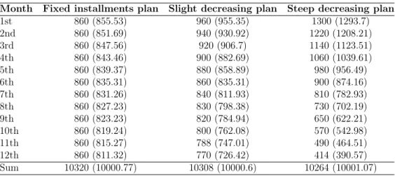
Table 1: Monthly nominal installments, their present values in parenthesis in $ under each plan
Month Fixed installments plan Slight decreasing plan Steep decreasing plan
1st 860 (855.53) 960 (955.35) 1300 (1293.7)
2nd 860 (851.69) 940 (930.92) 1220 (1208.21)
3rd 860 (847.56) 920 (906.7) 1140 (1123.51)
4th 860 (843.46) 900 (882.69) 1060 (1039.61)
5th 860 (839.37) 880 (858.89) 980 (956.49)
6th 860 (835.31) 860 (835.31) 900 (874.16)
7th 860 (831.26) 840 (811.93) 810 (782.93)
8th 860 (827.23) 830 (798.38) 730 (702.19)
9th 860 (823.23) 820 (784.94) 650 (622.21)
10th 860 (819.24) 800 (762.08) 570 (542.98)
11th 860 (815.27) 788 (747.01) 490 (464.51)
12th 860 (811.32) 770 (726.42) 414 (390.57)
Sum 10320 (10000.77) 10308 (10000.6) 10264 (10001.07)
As Table 1 shows, the sums of the present values of the monthly installments were similar (with only a few cents’ difference) across conditions. It also shows that, in the slight decreasing-installments plan (presented in the slight condition), the decrease in subsequent monthly installments was indeed small, with nominal installments slightly differing from those in the fixed-installments plan. In other words, we designed the slight decreasing-installments plan so as not to induce sufficient focus and, according to our propositions, to not significantly impact the evaluation of the fixed-installments plan but to control for the choice set’s increased cardinality. We expected an overall increase in the willingness to take out the loan in the slight condition compared to
the flat condition, since we would pick up people who would only take out the loan with this slight decreasing-installments plan.
In the third, steep condition, the loan was also offered in a steep decreasing- installments plan alongside the fixed-installments plan, as presented in the third column of Table 1 (again with equal present values between the two plans). We designed the steep decreasing-installments plan to induce a significant increase in focus, due to which (as laid out in the model section) people would be less likely to take out the fixed-installments plan in this condition than in the other two conditions.
We had no specific expectation as to whether or how the preference for a decreasing plan (be it slight or steep) would differ between the slight and the steep conditions.
Nevertheless, we expected that if the preference for the decreasing plan were stable across the slight and steep conditions, then a reduced preference for fixed-installments would result in an overall decrease in the willingness to borrow between the steep and the other two conditions.
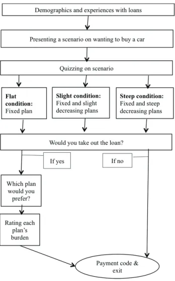
Fig 1 summarizes the study flow. Subjects first answered demographic questions, followed by a few questions about their experiences with loans (if any). Next they were presented a scenario that told them that they want to buy a car and, because they are $10,000 short, they are contemplating taking out a loan for that amount at a 6% annual interest rate. The loan would be repaid in twelve consecutive monthly installments. To minimize the effects of subjects’ real life income levels and other personal factors upon their choice, the scenario included a information about their financial and social-economic background. In this description they were married, had two school aged children and lived in the US. They were told that their monthly gross income is approximately $3,750, their spouse’s monthly gross income is approximately 75% of theirs, and they file their taxes jointly. We quizzed subjects to be sure that they understood to the task and remembered the key characteristics of their living situations. If they failed to pass the quiz, they reread the scenario and were quizzed again. Those who failed to pass the quiz after the maximum of three attempts proceeded with the study but were excluded from the analysis. After completing the quiz, subjects were presented with the offered loan plan(s) corresponding to their condition. While viewing the plans, they were asked if they would take out this loan.
If they answered no they finished and received their payment code. If they answered yes they were asked which plan they preferred (only in slight and steep conditions), and then to rate the burden of repayment under each plan they were presented. Then, these people also finished the study and received the payment code.
Figure 1: Experimental flow
3.1 Ethical statement
The focal experiment was conducted in line with guidelines of the Declaration of Helsinki (revised 1983) and local guidelines of the Faculty of Psychology at the University of Vienna. According to Austrian University Act (UG2002), only medical schools are required to have Ethical Committee or an Institutional Review Board (IRB). This implies we did not need an ethical approval to conduct this study.
Nevertheless, we obtained an on-line consent from all subjects and provided full disclosure about the study procedure. In order to ensure anonymity, we did not
collect any personal information about the enrolled subjects. Furthermore, subjects could discontinue participation at any point.
3.2 Subjects
Two hundred seventy-six subjects started the study, of which 41 were excluded, either due to attrition (12 subjects) or to failing the quiz (29 subjects). Of the two hundred thirty-five remaining, all lived in the US. We had seventy-two subjects in the flat, 80 in the slight and 83 in the steep conditions. The mean age in years differed across the three conditions, Welch’s F(2,151)=5.89, p≤0.01. The mean age was marginally greater in the slight (M=38.71, SD=12.80) than in the flat condition (M=34.14, SD=11.53), p≤0.1, and greater in the slight than in the steep condition (M=32.51, SD=10.24),p≤0.01. Note, we report Welch’s F statistics to account for the unequal variances in age across conditions. 56% of subjects were male and the median yearly gross income was below $55,000. Furthermore, 84% of subjects reported taking out at least one loan in the past 20 years. Find detailed sample demographics in S3 Appendix.
4 Results
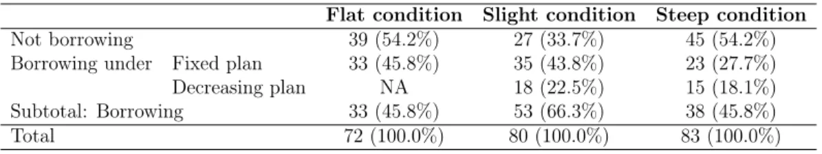
Our key prediction (derived from the proposition presented in the model section) was that the fixed-installments plan would be less preferred when it is offered along a steep decreasing-installments plan than when it is offered with a slight decreasing- installments plan (henceforth referred to as fixed, steep and slight plans, respectively) or alone. Table 2 presents the distribution of choice by condition. One can see from this table that the proportions of subjects choosing the fixed plan in the flat and slight conditions (46% and 44%, respectively) are almost equal, while there is a drop in choosing the fixed plan in the steep condition (28%).
Table 2: The distribution of choice in the three conditions N(%)
Flat condition Slight condition Steep condition
Not borrowing 39 (54.2%) 27 (33.7%) 45 (54.2%)
Borrowing under Fixed plan 33 (45.8%) 35 (43.8%) 23 (27.7%)
Decreasing plan NA 18 (22.5%) 15 (18.1%)
Subtotal: Borrowing 33 (45.8%) 53 (66.3%) 38 (45.8%)
Total 72 (100.0%) 80 (100.0%) 83 (100.0%)
To directly address our prediction we created a ’fixed preferred’ variable (1-fixed plan preferred, 0-else) and classified the conditions according to the presence of an
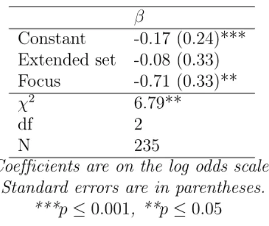
’extended set’ (1-slight and steep conditions, 0-flat condition) and ’focus’ (1-steep condition and 0-slight and flat conditions). The results of a binary logistic regression of fixed preferred on extended set and focus as predictors are presented in Table 3.
Note, extended set by focus is meaningless since we only had three conditions. This table shows that just offering the slight plan (i.e., extended set variable) does not change preference for the fixed plan, whereas the presence of a steep plan (i.e., focus variable) decreases preference for the fixed plan.
Table 3: Binary logistic regression (logit link function) of fixed plan preferred by extended set and focus
β
Constant -0.17 (0.24)***
Extended set -0.08 (0.33) Focus -0.71 (0.33)**
χ2 6.79**
df 2
N 235
Coefficients are on the log odds scale.
Standard errors are in parentheses.
***p≤0.001, **p≤0.05
Among those who would be willing to borrow (N=124), extended choice set and focus influenced the burden rating of the fixed plan in a way which was consistent with their effects on preference for the fixed plan. (Note, among the limitations we mention the pros and cons of eliciting burden ratings from only those who decided to borrow and not from everyone. We also discuss our reservations of these ratings in general.) Mean fixed plan’s burden was M=2.88, SD=0.93 in the flat, M=2.47, SD=0.91 in the slight, and M=2.82, SD=0.83 in the steep conditions. A two-way ANOVA of these ratings showed a significant effect of extended set, F(1,121)=4.23, p≤0.05, and a marginally significant effect of focus, F(1,121)=3.37,p≤0.1. Parameter estimates of these two effects show that extending the choice set decreases the fixed plan’s burden ratings by 0.41 on average (B=-0.41, SE=0.20), while focusing increases the burden ratings by 0.34 on average (B=0.34, SE=0.19). The values of these two estimates suggest that focusing almost entirely (by 83% on average) offsets the decrease in the perceived burden of the fixed plan induced by extending the set.
We argue that the choice dynamics attributed to focusing stem from the presence of the steep plan. This is because the steep plan shifts preference towards not borrowing from the fixed plan. To put it differently, instead of shifting from the fixed plan to the decreasing plan, people choose not to borrow at all. This is supported with the finding that we cannot find difference between the proportions of subjects of selecting either decreasing plans (slight or steep), binomial test of proportions, z=0.70, p=0.48, two-tailed.
To directly address this underlying mechanism, we restrict the sample to the slight and steep conditions (80 and 83 subjects, respectively) and test whether not borrowing was preferred relative to the fixed plan more in the steep than in the slight condition.
For this, we perform a multinomial logistic regression of ’behavior’ (not borrowing, borrowing under the fixed plan or borrowing under the decreasing plan) on condition (slight and steep). The model is significant,χ2(2)=7.27,p ≤0.05, and shows that subjects in the steep condition compared to subjects in the slight condition are more likely to choose not borrowing over the fixed plan,β=0.93, SE=0.36,p≤0.01. At the same time, however, there is no difference between these conditions in the probability of choosing the decreasing plan over not borrowing, nor of choosing the decreasing plan over the fixed plan.
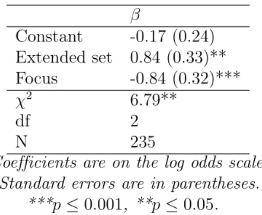
We anticipated that focusing offsets the effect of increasing the choice set’s cardinality (i.e., adding the slight plan) if the third option puts attention back onto the loan’s cost. If this were the case, the increased willingness to borrow in the extended set of fixed and slight decreasing plans could be offset by exchanging the slight decreasing plan to a steep decreasing plan. To test this prediction we performed a binary logistic regression of borrow (1-borrow, 0-not borrow) on extended set and focus, including the whole sample (N=235). As one can see from Table 4, increasing the choice set’s cardinality (i.e., extended set variable) does increase the willingness to borrow, while the presence of the steep decreasing plan (i.e., focus variable) decreases the likelihood of borrowing with almost identical odds.
5 Discussion
Building on theoretical predictions of Bakó et al. [17] we employed the model of focusing by Kőszegi and Szeidl [15], and show its applicability in examining a focusing illusion driven choice dynamics in a ternary set of intertemporal sequences. Adopting this framework we demonstrated how focus on the loan’s benefit (i.e., receiving the money) can be dampened by extending the choice set such that the difference in
Table 4: Binary logistic regression (logit link function) of borrowing by extended set and focus
β
Constant -0.17 (0.24) Extended set 0.84 (0.33)**
Focus -0.84 (0.32)***
χ2 6.79**
df 2
N 235
Coefficients are on the log odds scale.
Standard errors are in parentheses.
***p≤0.001, **p≤0.05.
salience between certain attributes (i.e., representing benefit and costs) is decreased.
In other words, attributes that were salient and more focused upon in the binary choice set become less so in a choice triplet if the third alternative induces sufficient focus. Our results suggest that focusing in a ternary choice set can play out such that it counteracts focusing effects observed in a binary choice set, and it can also offset the effect of increasing choice set’s cardinality.
When the choice triplet included the steep decreasing-installments plan, preference for the fixed-installments plan dropped compared to when – in addition to the option of not borrowing – the choice set included a slight decreasing-installments plan. Here people shifted their preferences from the fixed-installments plan to not borrowing. Furthermore, increased focusing due to the presence of the steep decreasing-installments plan offset the increased overall willingness to borrow caused by adding the slight decreasing-installments plan.
These choice dynamics were consistent with the burden ratings of making repay- ments under the fixed-installments plan in the three conditions. While just extending the choice set (i.e., adding the slight plan) decreased the perceived burden of the fixed-installments plan, exchanging the slight plan to a steep decreasing-installments plan put back these ratings to the original level observed in a binary choice set. This implies that, while more choices led to increased borrowing (due to picking up those who prefer borrowing under the slight decreasing-installments plan) and to a decreased perceived burden of the fixed-installments plan, exchanging the slight plan with a steep decreasing-installments one shifts preference from the fixed-installments plan to not borrowing, and also increases the perceived burden of the fixed–installments plan.
At the same time however, exchanging the slight with the steep decreasing-installments plan does not impact the preference of either decreasing plan.
We propose that these dynamics resulted because the steep decreasing-installments plan raised attention on the loan’s costs by making the fixed-installments plan with the salient benefit less attractive. This observed dynamics suggest that by using the model of focusing [15], one can strategically design the choice set so that under- weighted attributes become salient, making the alternative with the concentrated benefit seem less attractive. This mechanism could be exploited in situations where one would like to “sober” the decision-maker from being overly impressed by an option with a concentrated benefit. This is in line with the research agenda on choice architecture (e.g., [18]) advocating designing choice sets that work around people’s biases.
Although we used hypothetical loan decisions to demonstrate a focus driven choice dynamics, we conjecture that the same dynamics would be present in other choices between sequences of intertemporal outcomes. Specifically, where people are offered intertemporal sequences where one alternative includes a concentrated benefit (or cost) in one time point, people may attend more to, and thus overweight, this attribute.
Our results suggest that focusing could be dampened by adding an alternative that decreases the relative advantage of the looming attribute.
Consider, for instance, a choice between receiving pension savings in a lump-sum or in an annuity (i.e., equal size payoffs for a given time period). Because of focusing, the decision-maker may overly focus on the large lump-sum and underweight the attributes where he would receive the small and dispersed pay-offs of the annuity, leading him to opt for the former. Our findings suggest that an alternative annuity- payment plan with decreasing pay-offs could dampen the focusing biased choice. This is because the relative salience of the first attribute (i.e., receiving the lump sum) would be decreased if further attributes (i.e., receiving the annuity-payment) became more salient.
Obviously, any research such as ours where the choice elicitation procedure is is not payoff compatible has limitations. Specifically, some studies find inconsistent behavior across hypothetical and incentivized decisions (see, [45], [16]). In our study, subjects were paid a fixed fee so that their pay-offs were not contingent upon their choices. Because of this, people might have made less conservative choices, so that our results may have limited applicability to real life choices where a loan (or any) decision has serious monetary consequences on one’s welfare. Nevertheless, we argue that the observed cognitive mechanism which made people focus more on the loan’s costs should be the same whether or not payments depend on the choice.
Additionally, perhaps, we should have addressed the preference shift from the
fixed-installments plan to not borrowing using a within-subjects instead of a between- subject design. The within-subject design could, however, lead to people trying to be consistent in their choices instead of revealing their "true" preferences.
Furthermore, perhaps we could have asked everyone (including those who did not want to borrow) to rate the burden of the presented plans. This way we could have tested whether those not wanting to borrow perceived the plans as greater burden.
Nevertheless, the validity of these burden ratings may raise some doubts as they may reflect to some kind of ex post justification of the behavior instead of ”true" ratings.
Despite its weaknesses and limitations, our study demonstrates that it is possible to raise awareness of previously under-weighted attributes by adding alternatives that increase the salience of these attributes. This mechanism can be exploited in various real life decisions on intertemporal sequences where people may be prone to focus more on attributes in which their options differ more, and make choices affected by the focusing illusion.
Acknowledgments
We thank Gábor Neszveda for helpful comments. In addition, we are grateful for comments and suggestions from attendants at TIBER13, the Wien-Cologne Seminar, the GSS seminar at Tilburg University, and the MLSE Seminar at Maastricht University.
Supporting Information
S1 Appendix. Proofs
Assuming (without loss of generality) that ut(0) = 0 for all t, then over the choice set from the flat condition we have:
∆t(CF) =
(u0(L) t= 0
|δtut(−cf)| 0< t≤T
and over the choice set of the decreasing condition (or, substitutingS for D in the following, the slight condition):
∆t(CD) =
u0(L) t= 0
|δtut(−cd,t)| 0< t < kd−1
|δtut(−cf)| kd< t≤T
Theorem. The focus-weighted utility of cF is smaller in CD ={c0, cF, cD} than in CF ={c0, cF}.
Proof Letkd be the point, as defined in the text, where the decreasing-installments plan crosses over the fixed-installments plan. Then:
U˜(cF, CF)−U˜(cF, CD) =
T
X
t=0
δtg(∆t(CF))ut(−cf)−
T
X
t=0
δtg(∆t(CD))ut(−cf)
=
T
X
t=0
δtut(−cf)[g(∆t(CF))−g(∆t(CD))]
=
kd−1
X
t=1
δtut(−cf)[g(|δtut(−cf)|)−g(|δtut(−cd,t)|)]
>0
The final equality holds because ∆t(CF) = ∆t(CD)except for t= 1, . . . , kd−1. Since ut(·) and g(·)are strictly increasing and cd,t ≥cf for t = 1, . . . , kd−1, we have that g(|δtut(−cf)|)≤g(|δtut(−cd,t)|)with strict inequality for t= 1. Thus, the above sum
is strictly positive.
Proposition. If cD is more decreasing than cS then the focus-weighted utility of cF is smaller in CD ={c0, cF, cD} than in CS ={c0, cF, cS}.
Proof. Proceeding as with the previous proof, and noting that cd,t ≥ cf, cs,t when t= 1, . . . , kd−1 with strict inequality for t= 1:
U˜(cF, CS)−U˜(cF, CD) =
T
X
t=0
δtg(∆t(CS))ut(−cf)−
T
X
t=0
δtg(∆t(CD))ut(−cf)
=
ks−1
X
t=1
δtg(|δtut(−cs,t)|)ut(−cf) +
kd−1
X
t=ks
δtg(|δtut(−cf)|)ut(−cf)
−
kd−1
X
t=1
δtg(|δtut(−cd,t)|)ut(−cf)
=
ks−1
X
t=1
δtut(−cf)[g(|δtut(−cs,t)|)−g(|δtut(−cd,t)|)]
+
kd−1
X
t=ks
δtut(−cf)[g(|δtut(−cf)|)ut(−cf)−g(|δtut(−cd,t)|)]
>0
S2 Appendix. Experimental material
Demographics
1. Your year of birth: . . . 2. Are you:
• male
• female 3. Are you:
• African American
• Asian
• Caucasian
• Hispanic
• Other, please specify . . . 4. Your highest level of education
• Some high school or no high school
• High school graduate
• Trade school/some college/associate degree
• Advanced degree 5. Are you currently
• Unemployed
• Employed part-time
• Employed full-time
• Self-emplyoed
• Retried
• Other, please specify . . . 6. Your early income before taxes
• Under $30,000
• Between $30,001 and $55,000
• Between $55,001 and $95,000
• Over $95,001
7. Where do you currently live?
• City
• Town
• Small town
• Village
• Farm
8. Your religion
• Atheist or agnostic
• Buddhist
• Catholic
• Jewish
• Muslim
• Protestant
• Other, please specify . . . 9. In which country were you born?
• USA
• Other, please specify . . .
10. In the past twenty years have you ever taken out a loan from a financial institution? Only think about loans you took out from a bank, or any other financial institutions. DO NOT think about personal loans you received from your friends, family or other people.
• Yes, more than once
• Yes, only once
• No
Experiences with the loan
(For only those who answered yes to question #10)
Please recall the MOST RECENT LOAN you made and answer the following questions about this loan.
1. When (which year) did you take out this loan? Please provide your best guess:
. . .
2. What was the duration of this loan? That is, for how long do you or did you have to make payments on it? Please provide your best guess: . . .
3. What was the size of the loan in $? That is, how much money did you take out? Please provide your best guess: . . .
4. What was this loan for? That is, what did you purchase from this loan? Please briefly describe it with your own words‚ . . . .
5. Are you still repaying this loan?
• Yes
• No
6. What happened to this loan?
• I am still repaying this loan
• I paid it off
• I defaulted on it (did not make scheduled payments)
• Other, please specify . . .
7. Have you had or did you ever have hardships with making repayments on this loan?
• No, I never had any hardships making payments on this loan
• Yes, every now and then I had minor hardships making payments on this loan
• Yes, every now and then I had great hardships making payments on this loan
• Yes, making payments on the loan gave me slight, but permanent hardship
• Yes, making payments on the loan gave me great, but permanent hardship 8. This most recent loan was the largest loan I have taken out in the past twenty
years.
• Yes
• No Scenario
Please read this story very carefully
Imagine that you want to purchase a car. After a long and careful selection you have found a car that perfectly fits your needs and goals. However, you are $10,000 short,
You live in a town in the US, you are married, your spouse also makes money and you are raising two school-aged children. You are earning $45,000 per year before tax (which gives you approximately $3,750 per month before tax) and your spouse makes approximately three-fourths (i.e., 75%) of your income. You always file your taxes jointly with your spouse and both of your jobs are secure, at least for the next couple of years.
You research potentially interesting loans on the Internet. It seems that you are eligible to take out $10,000. You can get this loan on a 6% yearly interest rate. You also learn from the web that the banks would give you 6% yearly, nontaxable interest for your money deposits. Moreover, there is no inflation in your country.
If you read and understood this story please click on continue.
Quiz on scenario
1. In this story you are:
• Married with no children
• Maried with children
• Unmarried with a child
• Unmarried with no children
2. What is your yearly income (before taxes) in the story?
• Between $30,000 and $40,000
• Between $40,001 and $50,000
• Between $50,001 and $600,00
• Between $60,001 and $70,000 3. How do you file your taxes in the story?
• Alone
• Jointly with spouse
• This was not mentioned Flat/Slight/Steep conditions
The dealership where you are considering buying the car has a financing department is offering you the $10,000 loan with a 6% yearly interest rate. This bank offers you
a choice between two repayment plans. The two plans are identical in how much you end up paying for the loan and also in how much profit the bank makes on them.
The first plan is called the ’fixed-installments plan’ because you would have to pay the same amount every month for the entire duration. In this flat plan you would pay $860 a month from the day you took out the loan and would repeat this payment on the same day of every months for the next 12 months.
The second plan is called the ’decreasing-installments plan’ because you would have to pay a greater amount at the beginning and the size of the monthly payment would decrease over time. In this decreasing plan you would pay the first installment a month from the day you took out the loan and would repeat this payment on the same day of every months for the next 12 months.
The financial department also informs you about the procedure.
On the day you sign the contract, they would pay $10,000 towards your purchase of the selected car, and you then commit to paying the monthly installments on the same day of each month for the next 12 months. For a better understanding, they show you the following chart detailing what would happen in the following 12 months if you took out one of the loan plans (or if you did not take out the loan).
Visual presentation of plans
(Note, plans were presented throughout the whole study)
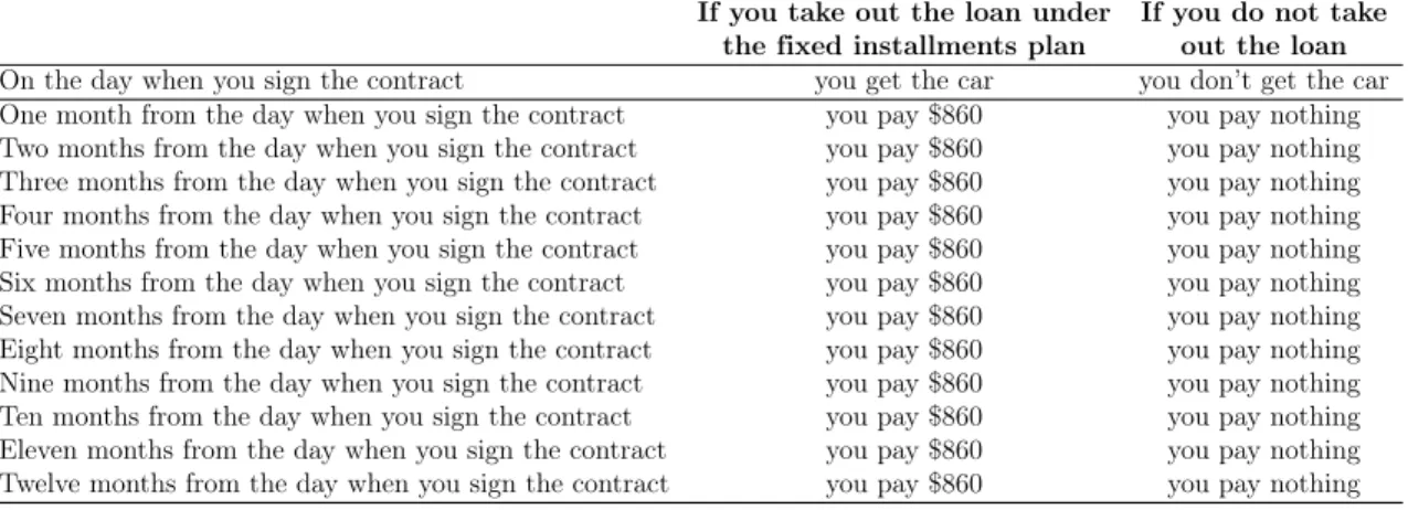
Table S2.1: Visual presentation of the choice set in the flat condition
If you take out the loan under the fixed installments plan
If you do not take out the loan On the day when you sign the contract you get the car you don’t get the car One month from the day when you sign the contract you pay $860 you pay nothing Two months from the day when you sign the contract you pay $860 you pay nothing Three months from the day when you sign the contract you pay $860 you pay nothing Four months from the day when you sign the contract you pay $860 you pay nothing Five months from the day when you sign the contract you pay $860 you pay nothing Six months from the day when you sign the contract you pay $860 you pay nothing Seven months from the day when you sign the contract you pay $860 you pay nothing Eight months from the day when you sign the contract you pay $860 you pay nothing Nine months from the day when you sign the contract you pay $860 you pay nothing Ten months from the day when you sign the contract you pay $860 you pay nothing Eleven months from the day when you sign the contract you pay $860 you pay nothing Twelve months from the day when you sign the contract you pay $860 you pay nothing
Table S2.2: Visual presentation of the choice set in the slight condition
If you take out the loan under the fixed installments plan
If you take out the loan under the decreasing
installments plan
If you do not take out the loan On the day when you sign the contract you get the car you get the car you don’t get the car One month from the day when you sign the contract you pay $860 you pay $960 you pay nothing Two months from the day when you sign the contract you pay $860 you pay $940 you pay nothing Three months from the day when you sign the contract you pay $860 you pay $920 you pay nothing Four months from the day when you sign the contract you pay $860 you pay $900 you pay nothing Five months from the day when you sign the contract you pay $860 you pay $880 you pay nothing Six months from the day when you sign the contract you pay $860 you pay $860 you pay nothing Seven months from the day when you sign the contract you pay $860 you pay $840 you pay nothing Eight months from the day when you sign the contract you pay $860 you pay $830 you pay nothing Nine months from the day when you sign the contract you pay $860 you pay $820 you pay nothing Ten months from the day when you sign the contract you pay $860 you pay $800 you pay nothing Eleven months from the day when you sign the contract you pay $860 you pay $788 you pay nothing Twelve months from the day when you sign the contract you pay $860 you pay $770 you pay nothing
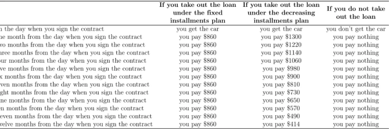
Table S2.3: Visual presentation of the choice set in the steep condition
If you take out the loan under the fixed installments plan
If you take out the loan under the decreasing
installments plan
If you do not take out the loan On the day when you sign the contract you get the car you get the car you don’t get the car One month from the day when you sign the contract you pay $860 you pay $1300 you pay nothing Two months from the day when you sign the contract you pay $860 you pay $1220 you pay nothing Three months from the day when you sign the contract you pay $860 you pay $1140 you pay nothing Four months from the day when you sign the contract you pay $860 you pay $1060 you pay nothing Five months from the day when you sign the contract you pay $860 you pay $980 you pay nothing Six months from the day when you sign the contract you pay $860 you pay $900 you pay nothing Seven months from the day when you sign the contract you pay $860 you pay $810 you pay nothing Eight months from the day when you sign the contract you pay $860 you pay $730 you pay nothing Nine months from the day when you sign the contract you pay $860 you pay $650 you pay nothing Ten months from the day when you sign the contract you pay $860 you pay $570 you pay nothing Eleven months from the day when you sign the contract you pay $860 you pay $490 you pay nothing Twelve months from the day when you sign the contract you pay $860 you pay $414 you pay nothing
1. First, think about this loan and indicate whether you would take it out or not
• Yes, I would take out this loan. If you select yes we will ask you later to specify which plan you would select.
• No, I would not take out this loan.
Only those answered “yes” on the previous answer:
2. Please indicate which plan you would prefer.
• Fixed-installments plan
• Decreasing-installments plan
3. Now, on the following scale please evaluate the burden of the fixed-installments plan. Think about the potential monthly hardship of paying back the loan under this plan.
• Not a burden at all
• A little bit of a burden
• A moderate burden
• A great burden
• An extreme burden
4. Now, on the following scale please evaluate the burden of the decreasing- installments plan. Think about the potential monthly hardship of paying back the loan under this plan.
• Not a burden at all
• A little bit of a burden
• A moderate burden
• A great burden
• An extreme burden
Thanks and good bye. This is your completion code: . . . (random number generated)
S3 Appendix. Additional analysis
Detailed demographics
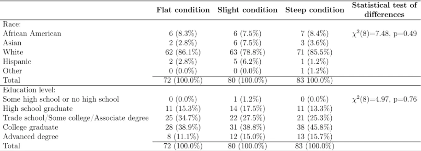
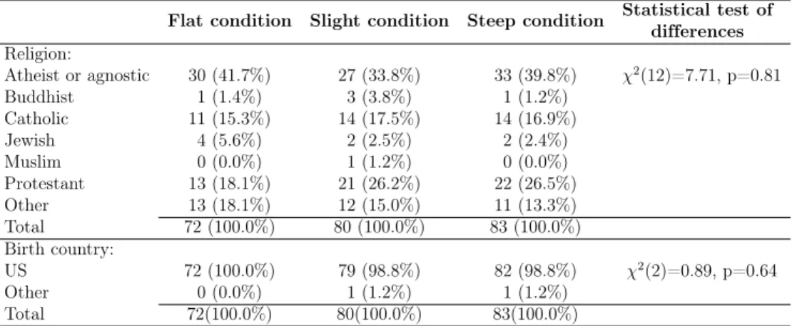
From Table S3.1 through Table S3.3 one can see that there are differences in race, education level, employment, living place, religion and country of birth across the three conditions. The majority of the sample is white, has some college or an associate degree, lives in cities or towns and was born in the US. Approximately half of the participants are employed full time and report as atheist or agnostic.
Table S3.1: Race and educational level distributions in the three conditions N (%)
Flat condition Slight condition Steep condition Statistical test of differences Race:
African American 6 (8.3%) 6 (7.5%) 7 (8.4%) χ2(8)=7.48, p=0.49
Asian 2 (2.8%) 6 (7.5%) 3 (3.6%)
White 62 (86.1%) 63 (78.8%) 71 (85.5%)
Hispanic 2 (2.8%) 5 (6.2%) 1 (1.2%)
Other 0 (0.0%) 0 (0.0%) 1 (1.2%)
Total 72 (100.0%) 80 (100.0%) 83 100.0%)
Education level:
Some high school or no high school 0 (0.0%) 1 (1.2%) 0 (0.0%) χ2(8)=4.97, p=0.76
High school graduate 11 (15.3%) 14 (17.5%) 11 (13.3%)
Trade school/Some college/Associate degree 25 (34.7%) 22 (27.5%) 21 (25.3%)
College graduate 28 (38.9%) 31 (38.8%) 38 (45.8%)
Advanced degree 8 (11.1%) 12 (15.0%) 13 (15.7%)
Total 72 (100.0%) 80 (100.0%) 83 (100.0%)
Table S3.2: Employment status and living place distributions in the three conditions N (%)
Flat condition Slight condition Steep condition Statistical test of differences Employment status:
Full-time 40 (55.6%) 44 (55.0%) 43 (51.8%) χ2(12)=7.72, p=0.81
Part-time 13 (18.1%) 10 (12.5%) 14 (16.9%)
Self-employed 7 (9.7%) 6 (7.5%) 8 (9.6%)
Retried 1 (1.4%) 3 (3.8%) 2 (2.4%)
Student 1 (1.4%) 1 (1.2%) 4 (4.8%)
Unemployed 10 (13.9%) 15 (18.8%) 10 (12.0%)
Other 0 (0.0%) 1 (1.2%) 2 (2.4%)
Total 72 (100.0%) 80 (100.0%) 83 (100.0%)
Living place:
City 31 (43.1%) 36 (45.0%) 45 (54.2%) χ2(10)=7.72, p=0.66
Town 23 (31.9%) 22 (27.5%) 20 (24.1%)
Small town 9 (12.5%) 17 (21.2%) 14 (16.9%)
Village 4 (5.6%) 2 (2.5%) 1 (1.2%)
Farm 4 (5.6%) 2 (2.5%) 2 (2.4%)
Other 1 (1.4%) 1 (1.2%) 1 (1.2%)
Total 72(100.0%) 80(100.0%) 83(100.0%)
Table S3.3: Religion and birth country distributions in the three condition N (%)
Flat condition Slight condition Steep condition Statistical test of differences Religion:
Atheist or agnostic 30 (41.7%) 27 (33.8%) 33 (39.8%) χ2(12)=7.71, p=0.81
Buddhist 1 (1.4%) 3 (3.8%) 1 (1.2%)
Catholic 11 (15.3%) 14 (17.5%) 14 (16.9%)
Jewish 4 (5.6%) 2 (2.5%) 2 (2.4%)
Muslim 0 (0.0%) 1 (1.2%) 0 (0.0%)
Protestant 13 (18.1%) 21 (26.2%) 22 (26.5%)
Other 13 (18.1%) 12 (15.0%) 11 (13.3%)
Total 72 (100.0%) 80 (100.0%) 83 (100.0%)
Birth country:
US 72 (100.0%) 79 (98.8%) 82 (98.8%) χ2(2)=0.89, p=0.64
Other 0 (0.0%) 1 (1.2%) 1 (1.2%)
Total 72(100.0%) 80(100.0%) 83(100.0%)
Prior experiences with loans
Table S3.4 presents subjects’ prior loan counts in the past twenty years by condition.
As shown, there is no difference between conditions in reported prior loans,χ2(4)=7.27, p=0.12.
Table S3.4: Prior loans in the three conditions N(%)
Flat condition Slight condition Steep condition Total
No prior loan 11 (15.3%) 9 (11.2%) 17 (20.5%) 37 (15.7%)
One prior 22 (30.6%) 14 (17.5%) 17 (10.5%) 53 (22.6%)
Multiple prior loans 39 (54.2%) 57 (71.2%) 49 (59.0%) 145 (61.7%)
Total 72 (100.0%) 80 (100.0%) 83 (100.0%) 235 (100.0%)
Next, those who reported taking out a loan in the past twenty years were asked about details of those loans. Those who reported multiple loans (145 participants) were asked to think about the most recent one. Table S3.5 presents the mean time elapsed in years since these loans were made and their mean size in US dollars. As one can see from this table there were no differences between the three conditions in the average years passed since the loans were made, nor in the mean size of the loans.
We also asked participants about the purpose of these loans. Responses are summarized in Table S3.6. Categorizes are used in line with Dezső and Loewenstein [46]. There are no significant differences in loan purposes across the three conditions,