Kész´ıtette:K˝oszegiBotondKözép-európaiEgyetemBudapest,2014.január ADVANCESINBEHAVIORALINDUSTRIALORGANIZATION MTADOKTORIÉRTEKEZÉS

(1)

MTA DOKTORI ´ERTEKEZ´ES

ADVANCES IN BEHAVIORAL INDUSTRIAL ORGANIZATION

K´esz´ıtette:

K˝oszegi Botond Közép-európai Egyetem

Budapest, 2014. janu´ar

(2)

Chapter 1 Introduction to Behavioral Economics

1.1 The Goal of this Dissertation

This dissertation familiarizes the reader with some recent advances in applied behavioral economics, especially behavioral industrial organization. To set up the stage for these newest developments, this chapter gives a general background and perspective on behavioral economics, and introduces the models of individual decisionmaking that will be used by the applied models.

1.2 What Is Behavioral Economics?

Psychology and economics—often also called “behavioral economics”—is not an easy field to define. In my view, it is not even really a field of economics at all, but more like a way of thinking about and doing research in any field. It is a mindset: the belief that economists should aspire to making assumptions about humans that are as realistic as possible, and hence that we should develop methods and habits to learn what is psychologically realistic.

What does this mindset entail? In a large part, it is not at all different from the mindset of the overwhelming majority of modern economics. We conceptualize economic phenomena by starting from individual behavior that is goal-driven: people try to understand their environment and to achieve their goals to the extent possible within the constraints they have. As in almost any field of economics, our aim is to understand how the goal-driven individual behavior plays out in different economic environments and what the welfare consequences are. Some of the habits and criteria we use in our teaching and research are therefore identical to those used by most economists.

We formalize ideas using mathematical models, in which decisionmakers are

(6)

often highly sophisticated. In our models and explanations, we highly value simplicity as well as generality, and in fact view this as a major advantage of many of the ideas we propose. And we recognize that markets and incentives play an important role in shaping behavior, that one of the main goals of economic analysis is to evaluate the performance of market institutions and policies, and that therefore it is important to test ideas using data on market behavior. All this means that psychology and economics is a field ofeconomics rather than psychology.

But there is a part of the habit and mindset of psychology and economics that is more new. Namely, we study more carefully and in more detail than most neoclassical economists what motivates people and how they go about maximizing their well-being. Our interest in “unpacking” how people might be thinking about and making decisions in turn implies an attentiveness and open-mindedness toward exploring behavior through experiments and surveys, and especially toward research in psychology, the other social sciences, and the brain sciences. What emerges from this investigation is a more nuanced, more detailed, and more accurate picture of individual economic actors than is typical in economics. But once we incorporate the more detailed knowledge of decisionmaking into our hypotheses, our goal is to understand economic consequences, especially market outcomes and welfare effects.

In some ways, the developments that led to the current field of behavioral economics are no different from those in game theory and information economics several decades ago. In both of these fields, researchers replaced previous—useful but simplistic—assumptions with more realistic and more detailed premises, and tremendously improved our understanding of economics as a result. Before the introduction of game theory into the field of industrial organization, many researchers thought of firm behavior in the market either in terms of perfect competition or in terms of monopoly. With game theory, it became possible to analyze intermediate cases more fully, and to understand how a firm’s strategic decisions depend on its information, resources, and the structure of the industry. Similarly, firm behavior has and still is often usefully conceptualized in terms of profit maximization (including in this dissertation).

Information economics, however, recognizes and assumes that a firm involves multiple individuals with possibly different motives and information. This allows a more nuanced understanding of the firm that is useful in many cir- cumstances, such as when trying to understand the boundaries of the firm and the labor market.

Psychology and economics does something similar, but where it expands or improves previous assumptions is in the realm of individual decisionmaking.

As with the above developments, this is more useful in some settings than

(7)

1.3. THE TASTE FOR IMMEDIATE GRATIFICATION 3

in others. This dissertation covers models of individual decisionmaking and applications that I believe are very important economically.

The historical development of behavioral economics can be categorized into three overlapping waves. In the first wave (which happened mostly in the 1970’s and 80’s), researchers identified systematic and important ways in which economic theory had been wrong, and suggested alternative ways of understanding behavior based on simple psychological principles. In the second wave (most of which started in the 90’s, and which is still going on today), economists formally modeled some of the alternatives, and established their empirical importance in the laboratory and the field. Finally, the third wave (most of which started in the 2000’s) involves full integration of the new psychologically based models into economic analysis, to address the same questions economists have always been interested in: how individual behavior plays out in organizations and markets, what the welfare consequences are, and how policy should respond to market outcomes.

The applications in this dissertation belong solidly in third-wave behavioral economics. They are built on a simple common principle of an asymmetry between consumers and firms. On the one hand, individual consumers are likely to be subject to the psychological phenomena documented by psychologists and behavioral economists. Hence, we assume that consumers exhibit these phenomena when making decisions in the marketplace. On the other hand, firms face incentives to maximize profits and have substantial resources and can create complex systems to make this happen. To capture this in an extreme way, we assume that they do not exhibit the psychological phenomena in question at all, but instead act as classical profit-maximizing firms.

The next two sections introduce the models of consumer behavior that will be used in later chapters. I introduce the taste for immediate gratification, which will be used in Chapter 2, in the next section. Then, I introduce loss aversion, which will be used in Chapters 3 and 4.

1.3 The Taste for Immediate Gratification

This section formalizes the taste for immediate gratification, and possible naivete regarding this taste, as modeled using the β-δ approach by Laibson (1997) and O’Donoghue and Rabin (1999). While I present some evidence as a way of motivating the model, I do not attempt to cover the broad array of evidence that has been accumulated over the years in favor of the model. For excellent reviews of the evidence, see Rabin (1998) and DellaVigna (2009).

(8)

0.0 0.2 0.4 0.6 0.8 1.0

1975 1980 1985 1990 1995 2000

δ

Year of Publication

Economics 119, Spring 2006 Source: Shane Frederick, conference talk

Figure 1.1: Estimated Annual δ’s from Economics Research

1.3.1 Introduction: The Need to Move Beyond Exponential Discount- ing

The standard theory for modeling intertemporal choices in economics is Samuel- son’s exponential-discounting model. In a version of this model, an agent making a decision at timet aims to maximize

u_t+δu_t+1+δ²u_t+2+· · ·=X

τ≥t

δ^τ−tu_τ,

whereuτ is the instantaneous utility at timeτ andδis the agent’sdiscount factor. The discount factor measures the proportional discount the agent applies to any one-period delay: instantaneous utility at any time is worth δ times as much as instantaneous utility in the previous period. In this model, the single variable that captures intertemporal preferences is δ. So it is little wonder that economists have tried to estimate δ over the years. Taken from Freder- ick, Loewenstein and O’Donoghue (2002), Figure 1.1 illustrates estimates of annual δ’s from economics research in the years 1975-2002. As is clear from the figure, there is tremendous variation in the estimates.

(9)

That economists’ estimates of δ are all over the place could mean three things. It could mean that economists have not made much progress in con- verging on a good estimate of δ, and that we need much more research to figure out which estimates are right. It could also mean that the discount factor is wildly variable across different situations and populations in a way that follows no logical pattern, so that there is no hope in pinning down an even approximate value for it. I find it implausible that these explanations provide a full account for the dispersion in measured δ’s, and hence will take a third perspective (one that I will argue helps explain the data): that δ simply cannot be measured accurately because the exponential discounting model tries to cram too much into this single parameter. Exactly as Samuelson intended, the model is an excellent way of conceptualizing and thinking about the fact that people make intertemporal tradeoffs, and the discount factor is a useful

“summary statistic” for how much the decisionmaker cares about the future in the particular situation. But intertemporal choice is a reflection of many psychological processes, some of which are more conducive to patience and some of which are more conducive to impatience. In addition, these forces are relevant in different choice problems to different degrees, so an economist who ignores them and tries to fit a single parameter onto every situation will keep measuring a different δ each time. Hence, the exponential discounting model is not a good model to shed light on how behavior varies across situations, and understanding the underlying psychological processes better will help us understand the variation better. As the most important example, I study self-control problems in this dissertation.

1.3.2 Short-Run Desires Versus Long-Run Goals

This section discusses two types of motivation for the model of hyperbolic discounting I introduce in the next section, both covering the model’s basic features and illustrating its economic importance. First, when it comes to tradeoffs between now and the near future, people are quite impatient. Second, when it comes to tradeoffs between nearby future dates, people are much more patient.

Evidence on Impatience in Short-Run Decisions

I begin this section by describing evidence from a range of decisionmaking situations showing that individuals can be quite impatient when it comes to choices that implicate immediate pleasures and pains. A common and economically relevant example is the so-called payday effect: individuals who live

(10)

from paycheck to paycheck spend a lot of their income immediately after getting paid. Huffman and Barenstein (2005), for instance, document that the consumption of working households in the United Kingdom is 18% higher the week after their payday than the week before. This indicates that when they get paid, they are eager to consume, and do not care so much that they will be suffering a few weeks down the line when they run out of money. Moti- vated by the same hypothesis, Shapiro (2005) finds that the caloric intake of food-stamp recipients declines by 13-14% over the month, while expenditure on food declines by about 20% over the month (indicating that households switch to less expensive foods over the course of the month). Shapiro argues that a high degree of short-run impatience is the most likely explanation for his findings, and rules out some alternative possible explanations.¹

People’s impatience regarding consumption is reflected not only in their spending a lot of their available funds immediately after they receive it, but also in their eagerness to borrow from future income. One expensive form of short- term borrowing is through credit cards, and in countries where credit cards are widely available, credit-card debt tends to be quite high. For example, in the United States in January 2012, the amount of outstanding revolving debt held by households (most of which is credit-card debt) was $800.9 billion. That is about $6,975 per household, including households that do not carry revolving debt. As of November 2011, the average interest rate on credit-card accounts with debt was 12.78%.² And credit cards are among the cheaper forms of short-term credit. One of the most expensive forms of (legal) borrowing in the United States is from one’s upcoming paycheck. About 10 million people borrow money through payday loans, and do so at annualized compounded percentage rates often exceeding 1000%. Yet there are more payday-loan and check-cashing outlets in the United States than there are McDonald’s and Starbucks combined.

1 In an interesting—if somewhat sad—twist to the payday effect, Hastings and Wash- ington (2010) document that store pricing responds to the effect: in areas with a lot of food-stamp recipients (but not in other areas), prices rise at the time beneficiaries receive their food stamps. This reaction is especially relevant for the current dissertation. Chapters 2-4 study how profit-maximizing firms react to consumers’ psychological phenomena, and the paper by Hastings and Washington demonstrates in a compelling way that firms do this.

2Source for these statistics: http://www.federalreserve.gov/releases/g19/

current/. It is worth mentioning that households use credit cards not only for immediate consumption, but also for purchases such as durables. One of the main results of Section 2 is showing that such purchases can also be understood in terms of the taste for immediate gratification.

(11)

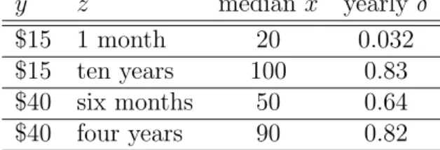
y z medianx yearly δ

$15 1 month 20 0.032

$15 ten years 100 0.83

$40 six months 50 0.64

$40 four years 90 0.82

Table 1.1: Some Findings of Thaler (1981) Patience in Decisions About the Future

All the situations discussed in the previous section implicate the possibility of immediate or near-immediate monetary receipts or consumption. I now argue that the high level of impatience people display is specific to such situations:

for similar tradeoffs that are further in the future, individuals tend to be more patient, so that exponential discounting cannot capture their attitudes toward delay for both short-run and long-run decisions.

The simplest way to see this is to carry out some thought experiments on the implications of applying the above type of impatience to intertemporal tradeoffs in general. Specifically, If a level of impatience that seems reasonable for short-run delays is applied to any delay of equal length, the implied level of impatience over long-run delays would be unreasonable. To illustrate, consider some simple arithmetic:

0.99^365×10 ≈ 1

8541609622012070 and 0.999^3×365×10≈ 1 57266.

If a person values tomorrow just one percent less than today—so that she ever-so-slightly prefers to put off an unpleasant task until tomorrow, even if that means the task becomes ever-so-slightly more difficult to perform—and applies the same preference to any one-day delay, she must value anything that happens in 10 years as totally insignificant relative to what happens today. Similarly, if she ever-so-slightly prefers to put off doing something from the morning to the evening, she must value today 57,266 times as much as 10 years from now (so she would not invest $100 to get $5 million in ten years).

These simple calculations suggest that the kind of short-run impatience found in the previous section cannot possibly describe intertemporal tradeoffs over longer horizons. Indeed, there is also direct evidence indicating that people are more impatient over short-term decisions than over long-term decisions. For instance, Thaler (1981) asked questions of the following form:

“What amount x makes you indifferent between $y today and $xin z time?”

(12)

5

0.0

4

0

5

10

15

time horizon (years)

Figure

l a . Discount Factor as a Function of Time Horizon (all studies)

although they did not interpret their results t h e same way.

If Read is correct about subadditive discounting, its main implication for economic applications may be to provide an alternative psychological underpin- ning for using a hyperbolic discount function, because most intertemporal decisions are based primarily on dis- counting from t h e present.17

17.4 few studies have actually found increasing discount rates. Frederick (1999) asked 228 respondents to imagine that they worked at a job that consisted of both leasant work (" ood days") and unpleasant work F b a d days") an$ to equate the attractiveness of having additional good days this year or in a future year. On average, respondents were indifferent between 20 extra good days this year, 21 the following year, or 40 in five years, im lying a one-year discount rate of

5

percent and a {ve-year discount rate of 15 percent A possible explanation is that a desire for improvement is evoked more strong1 for two successive years (this year and next) t

x

an for two separated years (this ear and five years hence). Rubinstein (2000) askedstudents in a political science class to choose between the following two payment sequences:

March 1 June 1 Sept 1 Nov 1 A: $997 $997 $997 $997

April 1 July1 Oct 1 Dec 1 B: $1000 $1000 $1000 $1000

Then, two weeks later, he asked them to choose between $997 on November 1 and $1000 on December 1. Fifty-four ercent of respondents referred $997 in Novernier to $1000 in Decem-

%er, but only 34 percent preferred sequence A to sequence B. These two results suggest increasing discount rates. To explain them Rubinstein specu-

time horizon (years)

Figu,re

l b . Discount Factor as a Function of Time Horizon (studies with avg. horizons >

1

year)

4.2 Other DU Anomalies

T h e DU model not only dictates that t h e discount rate should b e constant for all time periods; it also assumes that t h e discount rate should b e the same for all types of goods and all categories of intertemporal decisions. There are sev- eral empirical regularities that appear to contradict this assumption, namely:

(1)

_. ,

gains are discounted more than

_V

losses; ( 2 ) small amounts are discounted more than large amounts; ( 3 ) greater discounting is shown to avoid delay of a good than t o expedite its receipt;

( 4 ) in choices over sequences of outcomes, improving sequences are often preferred to declining sequences though positive time preference dic- tates t h e opposite; and (5) in choices over sequences, violations of indepen- dence are pervasive, and people seem to prefer spreading consumption over time in a way that diminishing marginal utility alone cannot explain.

4.2.1 The "Sign Effect" (gains are discounted more than losses)

Many studies have concluded that gains are discounted at a higher rate than losses. F o r instance, Thaler (1981)

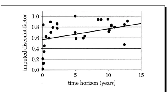
ments may have masked the differences in the timing of the sequence of dated amounts, while Figure 1.2: Estimated Discount Factors as a Function of the Time

Delay in Frederick, Loewenstein, and O’Donoghue (2002)

For each possible time delay z, one can calculate the equivalent yearly discount factorδ, and see howδ depends on the time delay. Table 1.1 gives some of Thaler’s findings. Clearly, the longer is the time delay, the larger is the implied yearly δ, indicating that individuals tend to become more patient on longer-run decisions.

Frederick and Loewenstein (1999) repeat the same exercise as Thaler, but do so using economists’ estimates of yearly discount factors rather than hy- pothetical choices. Figure 1.2 graphs the estimated yearly discount factor δ as a function of the delay in the decisionmaking situation based on which δ was estimated. Just like in Thaler’s case, the relationship is clearly and significantly positive. Hence, from analyses using different sources of data and different methods, the same pattern emerges over and over again: short-run discount factors are lower than long-run discount factors.

1.3.3 Modeling the Conflict Between Short-Run Desires and Long-Run Goals

Discounted Utility Function

As argued in detail in the previous section, evidence suggests that people discount nearby events quite heavily, but they are more patient for events

8

(13)

further away. Recent research has given rebirth to attempts to incorporate this pattern, and the interpersonal conflict it generates, formally into economics. In this section, I consider a modification of exponential discounting that captures these forces, and investigate some consequences of the new formulation.

Recall that Samuelson’s exponentially discounted utility model says that utility at time t is

u_t+δu_t+1+δ²u_t+2+δ³u_t+3+. . . .

Instead of Samuelson’s formulation, Laibson (1997) and O’Donoghue and Ra- bin (1999) assume that at time t, a person aims to maximize

u_t+βδu_t+1+βδ²u_t+2+βδ³u_t+3+. . .

with 0 < β ≤ 1. This is the hyperbolic discounting or (more precisely) quasi- hyperbolic discounting model. The extra parameterβthat applies to all future periods captures the extra discounting people apply to the future relative to the present due to their taste for immediate gratification. Since they apply β to all future periods equally, this means that they are relatively impatient when it comes to tradeoffs between the present and the future, but they are relatively patient when it comes to tradeoffs that occur in the future. And since β captures the extra discounting that occurs between the present and the future, it can be thought of as the short-run discount factor. Whenβ = 1, so that there is no extra discounting on the future, we get back to exponential discounting.

Analyzing the Model: Sophistication versus Naivete

To illustrate how to work with the hyperbolic discounting model, as well as to raise an additional issue, I demonstrate some of its implications in a simple decision. This analysis is based on O’Donoghue and Rabin (1999).

Consider a student’s decision of when to do a problem set. She could do it right after lecture (t = 0), when she remembers the material very well, or tomorrow (t= 1), when she remembers the material less well, or the day after tomorrow (t = 2), when she has forgotten everything. Because of this, the cost of doing the problem set increases, the later she does it. At date 0, the instantaneous disutility (immediate cost) of doing the problem set is 1. At date 1, the instantaneous disutility of doing the problem set is 3/2. At date 2, the instantaneous disutility of doing the problem set is 5/2. The student is a hyperbolic discounter with β = 1/2 and δ= 1.

To begin thinking about this example, first assume that the student can decide at time 0 when to do the problem set. This means, for example, that

(14)

she can decide at time 0 to do the problem set at time 1. Because she can decide what she will do in the future, we say that the student can commit or has access to commitment. For example, she could set up a study group that she cannot cancel later (or that is prohibitively costly to cancel later).

Since the student has different preferences at different points in time, we refer to her in multiple ways that reflect her changing preferences: we let self 0 be the period-0 incarnation of the student, self 1 her period-1 incarnation, and self 2 her period-2 incarnation. To decide when self 0 would like to do the problem set, we have to look at the discounted costs of doing it from the perspective of period 0:

• If the problem set is done in period 0, the discounted cost is 1.

• If the problem set is done in period 1, the discounted cost is ¹₂ · ³₂ = ³₄.

• If the problem set is done at period 2, the discounted cost is ¹₂ · ⁵₂ = ⁵₄. Because it minimizes the discounted cost of doing the problem set, self 0 commits to doing it in period 1. Intuitively, because of her taste for immediate gratification, the student prefers to delay—because she cares much more about the present than about the future, she is willing to put off the task even though she knows it will become harder. But because she is more patient when it comes to future tradeoffs, she does not want to delay more than one period.

Now suppose that the student has no access to a commitment technology.

So, in both period 0 and period 1, she freely decides whether she does the problem set then or later (at date 2, she has to do it if she has not already finished it). It would still be the case that self 0 wouldwant todo the problem set at time 1. Would she actually do it at time 1? To answer this, we look at discounted costs from the perspective of period 1:

• If the problem set is done in period 1, the discounted cost is ³₂.

• If the problem set is done in period 2, the discounted cost is ⁵₄.

So she now prefers to do the problem set at time 2. Because the student’s earlier preference for what she should do at a later point (her period-0 preference for doing the problem set at time 1) is different from what she wants to do when the time comes (her period-1 preference to delay doing the problem set), the student is dynamicallyinconsistent. This intertemporal conflict leads to a self-control problem: the student wants to exercise self-control tomorrow, but once tomorrow come she may not want to.

(15)

But given this conflict, when does the student actually do the problem set?

It turns out that with the information introduced so far, it is impossible to answer this question. To understand how the self-control problem plays out, we need to know whether the student is aware that she will change her mind in the future. There are two extreme assumptions one can make in this regard.

Naive decisionmakers are not aware of their own self-control problem—they persist in happily thinking that whatever they plan will actually be carried out by their later selves. Sophisticated decisionmakers, on the other hand, perfectly anticipate their future behavior—they do not harbor illusions about their ability to carry through plans. This means that they will try to take actions to make sure they stick with current plans. These two possible assumptions about the student’s self-awareness are very extreme, and most of us have features of both sophistication and naivete.

Now we are ready to analyze the student’s behavior, separately by their degree of sophistication. We start with a naive student. We have already calculated that self 0 would prefer to do the problem set at time 1, and since (being naive) she assumes she will behave “correctly” in the future, that is what she assumes she will do. Hence, she does not do the problem set at time 0, thinking, “Well, this is no big deal, I will just do it tomorrow...” We have also calculated that she does not do the problem set at time 1, so a naive student does the problem set in period 2.

Intuitively, since she believes that she will do the problem set before this will be too hard, she believes she cannot lose much by delaying. Next period, she again perceives the cost of delaying to be small, so she delays again.

Note that from the point of view of time 0, the student incurs a discounted cost of 5/4, higher than if she did the problem set in period 0. That is, the student does something she considers unambiguously bad for herself. This could not happen with exponential discounting: with exponential discounting, whatever self 0 thinks is the best thing to do, later selves will be willing to do.

Hence, the behavior of the naive student is not driven purely by impatience—

time inconsistency is implicated as well. That hyperbolic discounters often do things that they perceive as unambiguously bad for themselves is an important property of these models, and plays a central role in applications of hyperbolic discounting, including that in Chapter 2.

We now turn to sophisticated students. We know that if the student does not do the problem set in period 0, she does not do it in period 1, either. A sophisticated student realizes this, so she knows that if she does not do the problem set in period 0, she will not do it until period 2. Since (according to the above calculation) she prefers to do it in period 0 rather than in period 2, a sophisticated student does problem set in period 0.

(16)

Intuitively, a sophisticated student recognizes that if she delays, she will delay more. Since she knows that would be too costly, she reluctantly does the problem set at time 0.

As mentioned above, the most realistic assumption seems to be that most individuals are neither fully sophisticated, nor fully naive. How do we model such decisionmakers? O’Donoghue and Rabin (2001) assume that the agent believes with probability 1 that her future β will equal ˆβ. In this formulation, βˆ=βcorresponds to full sophistication, and ˆβ = 1 corresponds to full naivete.

Eliaz and Spiegler (2006) and Asheim (2008) assume that the agent has beliefs that put some probability on ˆβ = β, and the complementary probability on βˆ= 1. In some settings, Heidhues and K˝oszegi (2010a) (Chapter 2) allow for a person’s beliefs to be a full distribution.

1.4 Reference Dependence and Loss Aversion

This section introduces reference dependence and loss aversion, which will be used as the model of consumer behavior in Chapters 3 and 4. As in the case of hyperbolic discounting, I discuss some evidence as a way of motivating the model, but do not discuss the full array of evidence in favor of the model. For evidence, see Rabin (1998) and DellaVigna (2009).

1.4.1 An Illustration and an Introduction

Take a look at Figure 1.3 illustrating the Gradient Illusion. The central stripe in the illustration is actually uniform in color. Yet the part surrounded by a darker grey looks lighter than the part surrounded by a lighter grey. The illusion persists even after one has been told that the central stripe is of uniform color, after one has measured the color in Photoshop, and even if one has created the figure oneself.

This illusion illustrates the extent to which our brain tends to perceive things relative to other things. Just by putting these different background colors next to the central stripe, we can induce the brain to automatically make the comparison, and for that to dominate the judgment about the absolute color of the stripe. Even once you are fully convinced that this is an illusion, the central stripe still does notseemuniform in color. It is just hard to see it in any other way. More generally, in judging perceptive things such as brightness, loudness, or temperature, the stimuli are perceived in relation to some neutral point.

The tendency to compare stimuli to other stimuli extends to the economic

(17)

1.4. REFERENCE DEPENDENCE AND LOSS AVERSION 13

Figure 1.3: The Gradient Illusion. The central stripe has uniform color—yet it seems much lighter on the left side.

domain in a big-time way. We call this the phenomenon ofreference-dependent preferences: that the utility level we derive from an outcome depends in a major way on comparisons to certain “benchmark” outcomes orreference points—

not only on an absolute evaluation of the outcome itself. A large literature starting with Kahneman and Tversky (1979) is devoted to modeling reference- dependent preferences and its implications for economics.

1.4.2 Loss Aversion

The most important property of reference-dependent preferences is loss aversion—

people dislike losses relative to the reference point more than they like same- sized gains. I illustrate two kinds of evidence on loss aversion, that based on people’s willingness to trade their current position for another one, and that based on choices over risky gambles.

Loss aversion is manifested in the striking endowment effect documented first by Kahneman, Knetsch, and Thaler (1990, 1991) and subsequently by many other researchers: once a person comes to possess a good, she almost immediately values it more than before she possessed it. These experiments usually start by randomly giving half the subjects (often a class) mugs. These subjects become the “owners” or potential sellers, and the others are “non-

(18)

owners” or potential buyers. The owners are then asked to examine the mug and think about how useful it might be to them. They are also asked to pass their mug to the closest non-owner, so that they can examine it as well. This is an important part of the design, because it reduces the information asymmetry between owners and non-owners. Buying and selling prices are then elicited in an incentive-compatible way using the Becker-DeGroot-Marschak procedure (Becker, DeGroot and Marschak 1964). Prototypical experiments starting with Kahneman, Knetsch and Thaler (1990), have consistently found a major gap, with selling prices being about twice the buying prices.

The endowment effect—the fact that owners value a good more than other- wise identical non-owners—is usefully conceptualized as a case of loss aversion.

Individuals who are randomly given mugs treat the mugs as part of their reference levels or endowments, and consider not having a mug to be a loss.

Individuals without mugs consider not having a mug as remaining at their reference point, and getting a mug as a gain. Since people are more sensitive to losses than they are to same-sized gains, the sellers “value” the mug more:

by keeping the mug, they avoid a loss, whereas buyers would merely make a gain if they got the mug.

Another important manifestation of loss aversion is in attitudes toward risky gambles. For instance, most people would turn down an immediate fifty-fifty gain $550 or lose $500 gamble. This kind of risk aversion seems such an intuitively obvious fact that for a long time researchers have not even bothered to check it. But recently, Barberis, Huang and Thaler (2006) offered the gamble for real to MBA students, financial analysts, and even very rich investors (with median financial wealth over $10 million!). A majority of all these people, including 71% of the investors, rejected the gamble.

The standard economic explanation for people’s rejection of this gamble is risk aversion or (equivalently for our purposes) diminishing marginal utility of wealth. Indeed, diminishing marginal utility of wealth is an excellent assumption based on good psychology: people satisfy their most important needs and desires first and the less important ones only if they have something left over, so the first $1,000,000 in wealth generates more utility than the next

$1,000,000. This is a great explanation for large-scale risk aversion, such as the decision to take $4 million for sure rather than $10 million with probability one-half.

But most of the risky decisions we face are not in the $1 million range or even the $100,000 range. They are much smaller. And in a key article, Rabin (2000a) argued that expected-utility-over-wealth maximizers—who care only about final wealth outcomes—should not reject such a gamble unless they turn down phenomenally favorable larger risks. Since most people do take

(19)

many risks, expected utility is not a reasonable explanation for rejecting the small-scale gamble. Rabin’s mathematical argument centers around proving statements of the following form: “If an individual with expected utility over wealth turns down a fifty-fifty lose $l or gain $g gamble over a range of wealth levels, she also turns down a fifty-fifty lose $L or gain $G gamble,” where G is huge relative to L and Lis not that large (Gis infinite in some examples).

The argument proceeds by using that if a person turns down the g/l gamble for some wealth level, her marginal utility must diminish by some non-trivial amount over the range of the gamble. Using that this is the case for multiple wealth levels, we conclude that over the range of these wealth levels marginal utility diminishes quite a lot. But this implies extreme sensitivity to larger gambles.

Here is an illustration of the precise argument. Suppose Johnny is a classical utility maximizer with diminishing marginal utility of wealth who would turn down a fifty-fifty lose $500 or gain $550 bet for a non-trivial range of initial wealth levels. Let us take a concave, increasing utility function over wealth, u(·). Rejection of this bet means that

1

2u(w+ 550) + 1

2u(w−500)< u(w), which implies

u(w+ 550)−u(w)< u(w)−u(w−500).

But notice that by the concavity ofu(·),u(w)−u(w−500)<500·u⁰(w−500), and u(w+ 550)−u(w)>550·u⁰(w+ 550). Therefore,

500·u⁰(w−500)>550·u⁰(w+ 550), or

u⁰(w−500)> 11

10u⁰(w+ 550).

Now suppose Johnny was $1,050 poorer in lifetime terms. This is a very small change in lifetime wealth, equivalent to something less than $50 per year.

It is implausible that risk aversion would diminish significantly with such small changes in initial wealth, especially for decreases in wealth. If so, then by the same argument as above but now applied to a wealth level of w−1050,

u⁰(w−1550)> 11

10u⁰(w−500).

Combining the two

u⁰(w−1550)>

11 10

2

u⁰(w+ 550),

(20)

and by the same reasoning

u⁰(w−2100)>

11 10

2

u⁰(w).

But this implies that marginal utility for wealth skyrockets for larger decreases in wealth unless there are dramatic shifts in risk attitudes over larger changes in wealth: for every decrease of $1,050 in Johnny’s wealth, his marginal utility of wealth increases by a factor of 11/10. Doing this fifty times... If Johnny became $52,500 poorer in lifetime wealth—which is something less than $2,500 in pre-tax income per year, say—then he would value income at least 117 times (≈ ¹¹₁₀50

) as much as he currently does. While none of us know Johnny, we know this is a false fact about Johnny.

Furthermore, such a plummeting marginal utility of money leads to wild risk aversion over large stakes: if Johnny’s marginal utility of wealth increases by a factor of 117 if he were $52,500 poorer, for instance, then—even if he were risk neutral above his current wealth level—then Johnny would turn down a fifty-fifty lose $110,000 or gain $6.4 million bet at his current wealth level.³

By a similar calculation, if Johnny were risk neutral above his current wealth level but averse to 50/50 lose $10 / gain $11 bets below his current wealth level, then he would turn down a 50/50 lose $22,000 / gain $100 billion bet. Rabin gives many further numerical examples.

Since this kind of risk aversion is inconceivable (how many would turn down this last bet?), we can conclude that diminishing marginal utility of wealth cannot reconcile risk aversion over modest stakes with reasonable risk aversion over large stakes. And these results are just bounds, and vastly understate the severity of large-scale risk aversion implied by small-scale risk aversion.

So why do people reject a fifty-fifty lose $500 or gain $550 risk? Most likely because of loss aversion. They dislike the prospect of an unpleasant loss of

$500 much more than they like the prospect of a gain of $500. Loss aversion is not subject to the same critique as diminishing marginal utility over wealth because it does not assume that risk preferences over any level of wealth are determined by a single function. It could be that at any wealth level, a person dislikes a $500 loss much more than she likes a $550 gain—if her reference point is her current wealth. But this does not mean that her utility function is

3To get this number, I used that Johnny’s marginal utility at wealth levels below the current wealth minus $52,500 is at least 117 times that at his current wealth level. A

$110,000 loss is a loss of more than $55,000 extra. He cares about this extra loss at least 117 times as much than about gains from the current wealth level. So even a gain of 6,400,000<117×55,000 would not be enough to compensate him.

(21)

very concave overall, because it does not imply that her utility function must at the same time curve at each of these wealth levels.

In other words, loss aversion gets around the Johnny logic by assigning a special role to current wealth (or another reference point), and making a strong distinction between gains and losses. Because losses are much more painful than equal-sized gains are pleasant, it may well be that a gain of $550 is not as attractive as a loss of $500 is scary. But with loss aversion, it is not necessarily the case that a loss of an extra $500 is worse than the loss of the first $500—since both of these are losses. So the above logic breaks down.

1.4.3 The Reference Point

Predictions of reference-dependent preferences and loss aversion of course depend crucially on what we assume the reference point is. While many theories of reference-point determination have been proposed, the most frequently used theory in recent years is that of K˝oszegi and Rabin (2006). To motivate the key assumption in our model, I begin with an experiment. Abeler, Falk, G¨otte and Huffman (2011) gave students a menial task (entering data into the com- puter) to perform for a piece-rate. Students could work as long as they wanted.

The twist in the authors’ experiment was in how students were paid. After a student finished working, a random draw was made: with probability one- half, the student received what she earned in the task, and with probability one-half, she received a predetermined amount. For a randomly chosen half of the subjects, the predetermined amount was e3.50, and for the other half, it was e7.00. Subjects knew all these details of the experiment, including their own predetermined amount, in advance.

Abeler et al. (2011) found a striking difference in how much the two groups of students worked: the group whose predetermined amount wase3.50 tended to stop more when they earned e3.50, and the group whose predetermined amount was e7.00 tended to stop more when they have earned e7.00. In a sense, the predetermined amount became a target for how much to earn. This indicates that a subject’s recent expectations (i.e., probabilistic beliefs) about how much she might earn determine her reference point for earnings. Chapters 3 and 4 of the dissertation build on this assumption, first formalized by K˝oszegi and Rabin (2006). Other evidence also lends support to the expectations- based model. In a simple exchange experiment, Ericson and Fuster (2009) find that subjects are more likely to keep an item they had received if they have been expecting a lower probability of being able to exchange it, consistent

(22)

with the idea that their expectations affected their reference point.⁴ Crawford and Meng (2011) propose a model of cabdrivers’ daily labor-supply decisions in which cabdrivers have rational-expectations-based reference points (“tar- gets”) in both hours and income. Crawford and Meng show that by making predictions about which target is reached first given the prevailing wage each day, their model can reconcile the controversy between Camerer, Babcock, Loewenstein and Thaler (1997) and Farber (2005, 2008) in whether cabdrivers have reference-dependent preferences.

4 In an alternative experiment, Ericson and Fuster (2009) find that subjects are willing to pay 20-30 percent more for an object if they had expected to be able to get it with 80-90%

rather than 10-20% probability. In a similar experiment, however, Smith (2008) does not find the same effect.

(23)

Chapter 2 Exploiting Naivete about Self-Control in the Credit Market ¹

2.1 Introduction

Researchers as well as policymakers have expressed concerns that some contract features in the credit-card and subprime mortgage markets may induce consumers to borrow too much and to make suboptimal contract and repayment choices.² These concerns are motivated in part by intuition and evidence on savings and credit suggesting that consumers have a time-inconsistent taste for immediate gratification, and often naively underestimate the extent of this taste.³ Yet the formal relationship between a taste for immediate gratifica-

1This chapter is coauthored with Paul Heidhues, and appeared in the American Economic Review (2010), 100(5), pp. 2279-2303. Some features of real-life credit contracts we discuss in the paper no longer exist in the United States due to recently enacted regulations—also mentioned in the paper—that are very similar in spirit to the welfare-improving interventions we propose. Hence, our discussion of contract terms is most appropriate for the period ending around 2010.

2 See, for instance, Ausubel (1997), Durkin (2000), Engel and McCoy (2002), Bar-Gill (2004), Warren (2007), and Bar-Gill (2008).

3 Laibson, Repetto and Tobacman (2007) estimate that to explain a typical household’s simultaneous holdings of substantial illiquid wealth and credit-card debt, the household’s short-term discount rate must be higher than its long-term discount rate. Complementing this finding, Meier and Sprenger (2010) document that low and middle-income individuals who exhibit a taste for immediate gratification in experimental choices over monetary payments have more outstanding credit-card debt. Laibson et al. (2007) calculate that many households are made worse off by owning credit cards, so the fact that they get those cards suggests some degree of naivete about future use. Consistent with this idea, consumers overrespond to the introductory “teaser” rates in credit-card solicitations relative to the length of the introductory period (Shui and Ausubel 2004) and the post-introductory inter-

(24)

tion and consumer behavior and welfare in the credit market remains largely unexplored and unclear. Existing work on contracting with time inconsistency (DellaVigna and Malmendier 2004, K˝oszegi 2005, Eliaz and Spiegler 2006) does not investigate credit contracts and especially welfare and possible welfare-improving interventions in credit markets in detail. Furthermore, because borrowing on a mortgage or to purchase a durable good typically involves up-front effort costs with mostly delayed benefits, models of a taste for immediate gratification do not seem to predict much of the overextension that has worried researchers and policymakers.

In this paper, we provide a formal economic analysis of the features and welfare effects of credit contracts when some consumers have a time-inconsistent taste for immediate gratification that they may only partially understand.

Consistent with real-life credit-card and subprime mortgage contracts but (we argue) inconsistent with natural specifications of rational time-consistent theories, in the competitive equilibrium of our model firms offer seemingly cheap credit to be repaid quickly, but introduce large penalties for falling behind this front-loaded repayment schedule. The contracts are designed so that borrowers who underestimate their taste for immediate gratification both pay the penalties and repay in an ex-ante suboptimal back-loaded manner more often than they predict or prefer. To make matters worse, the same misprediction leads non-sophisticated consumers to underestimate the cost of credit and borrow too much—despite borrowing being for future consumption. And because the penalties whose relevance borrowers mispredict are large, these welfare implications are typically large even if borrowers mispredict their taste for immediate gratification by only a little bit and firms observe neither borrowers’ preferences nor their beliefs. Accordingly, for any positive proportion of non-sophisticated borrowers in the population, a policy of disallowing large penalties for deferring small amounts of repayment—akin to recent new US regulations limiting prepayment penalties on mortgages and certain interest charges and fees on credit cards—can raise welfare.

Section 2.2 presents our model. There are three periods, 0, 1, and 2. If the consumer borrows an amount c in period 0 and repays amounts q and r in periods 1 and 2, respectively, self 0, her period-0 incarnation, has utility c−k(q)−k(r), where k(·) represents the cost of repayment. Self 1 maximizes

est rate (Ausubel 1999), suggesting that they end up borrowing more than they intended or expected. Skiba and Tobacman (2008) find that the majority of payday borrowers default on a loan, yet do so only after paying significant costs to service their debt. Calibrations indicate that such costly delay in default is only consistent with partially naive time inconsistency. For further discussions as well as evidence for a taste for immediate gratification in other domains, see DellaVigna (2009).

(25)

2.1. INTRODUCTION 21

−k(q)− βk(r) for some 0 < β ≤ 1, so that for β < 1 the consumer has a time-inconsistent taste for immediate gratification: in period 1, she puts lower relative weight on the period-2 cost of repayment—that is, has less self- control—than she would have preferred earlier. Since much of the borrowing motivating our analysis is for future consumption, self 0 does not similarly discount the cost of repayment relative to the utility from consumption c.

Consistent with much of the literature, we take the long-term perspective and equate the consumer’s welfare with self 0’s utility, but the overborrowing we find means that self 1 and self 2 are also hurt by a non-sophisticated borrower’s contract choice. To allow for self 0 to be overoptimistic regarding her future self-control, we follow O’Donoghue and Rabin (2001) and assume that she believes she will maximize −k(q)−βk(r) in period 1, so that ˆˆ β satisfying β ≤βˆ≤1 represents her beliefs aboutβ.

The consumers introduced above can sign exclusive non-linear contracts in period 0 with competitive profit-maximizing suppliers of credit, agreeing to a consumption level c as well as a menu of installment plans (q, r) from which self 1 will choose. Both for theoretical comparison and as a possible policy in- tervention, we also consider competitive markets in which disproportionately large penalties for deferring small amounts of repayment are forbidden. For- mally, in a restricted market contracts must be linear—a borrower can shift repayment between periods 1 and 2 according to a single interest rate set by the contract—although as we discuss, there are other ways of eliminating disproportionately large penalties that have a similar welfare effect.

Section 2.3 establishes our main results in a basic model in which β and βˆ are known to firms. Since a sophisticated borrower—for whom ˆβ = β—

correctly predicts her own behavior, she accepts a contract that maximizes her ex-ante utility. In contrast, a non-sophisticated borrower—for whom ˆβ > β—

accepts a contract with which she mispredicts her own behavior: she believes she will choose a cheap front-loaded repayment schedule (making the contract attractive), but she actually chooses an expensive back-loaded repayment schedule (allowing firms to break even). Worse, because the consumer fails to see that she will pay a large penalty and back-load repayment—and not because she has a taste for immediate gratification with respect to consumption—

she underestimates the cost of credit and borrows too much. Due to this combination of decisions, a non-sophisticated consumer, no matter how close to sophisticated, has discontinuously lower welfare than a sophisticated consumer. This discontinuity demonstrates in an extreme form our main point regarding contracts and welfare in the credit market: that because the credit contracts firms design in response postulate large penalties for deferring repayment, even relatively minor mispredictions of preferences by borrowers can

(26)

have large welfare effects.

Given the low welfare of non-sophisticated borrowers in the unrestricted market, we turn to identifying welfare-improving interventions. Because in a restricted market borrowers have the option of paying a small fee for deferring a small amount of repayment, non-sophisticated but not-too-naive borrowers do not drastically mispredict their future behavior, and hence have higher utility than in the unrestricted market. Since sophisticated borrowers achieve the highest possible utility in both markets, this means that a restricted market often Pareto-dominates the unrestricted one. If many borrowers are very naive, a restricted market can be combined with an interest-rate cap to try to limit borrowers’ misprediction and achieve an increase in welfare.

The properties of non-sophisticated borrowers’ competitive-equilibrium contracts, and the restriction disallowing disproportionately large penalties for deferring small amounts of repayment, have close parallels in real-life credit markets and their regulation. As has been noted by researchers, the baseline repayment terms in credit-card and subprime mortgage contracts are typically quite strict, and there are large penalties for deviating from these terms. For example, most subprime mortgages postulate drastically increased monthly payments shortly after the origination of the loan or a large “balloon” payment at the end of a short loan period, and failing to make these payments and refinancing triggers significant prepayment penalties. Similarly, most credit cards do not charge interest on any purchases if a borrower pays the entire balance due within a short one-month grace period, but do charge interest on all purchases if she revolves even $1. To protect borrowers, new regulations restrict these and other practices involving large penalties: in July 2008 the Federal Reserve Board severely limited the use of prepayment penalties, and the Credit CARD Act of 2009 prohibits the use of interest charges for partial balances the consumer has paid off, and restricts fees in other ways. Oppo- nents have argued that these regulations will decrease the amount of credit available to borrowers and exclude some borrowers from the market. Our model predicts the same thing, but also says that this will benefit rather than hurt consumers—who have been borrowing too much and will now borrow less because they better understand the cost of credit.

In Section 2.4, we consider equilibria whenβis unknown to firms, and show that with two important qualifications the key results above survive. First, since sophisticated and non-sophisticated borrowers with the same ˆβ are now indistinguishable to firms, the two types sign the same contract in period 0.

This contract has a low-cost front-loaded repayment schedule that a sophisticated borrower chooses, and a high-cost back-loaded repayment schedule that a non-sophisticated borrower chooses. As before, even if a non-sophisticated

(27)

2.1. INTRODUCTION 23

borrower is close to sophisticated, the only way she can deviate from the front- loaded repayment schedule is by paying a large fee. Furthermore, we identify reasonable conditions under which consumers self-select in period 0 into these same contracts even if β and ˆβ are both unknown to firms. Second, while the restricted market does not Pareto-dominate the unrestricted one, we establish that for any proportion of sophisticated and non-sophisticated borrowers, if non-sophisticated borrowers are not too naive, then the restricted market has higher total welfare.

In Section 2.5, we generalize our basic model—in which a non-sophisticated borrower believes with certainty that her taste for immediate gratification is above β—as well as other existing models of partial naivete and allow borrower beliefs to be a full distribution F( ˆβ). We show that whether or not borrower beliefs are known, the qualitative predictions we have emphasized for non-sophisticated borrowers—overborrowing, often paying large penalties, and getting discretely lower welfare than sophisticated borrowers—depend not onF(β) = 0, but onF(β) being bounded away from 1. Since this condition is likely to hold for many or most forms of near-sophisticated borrower beliefs, our observation that small mispredictions have large welfare effects is quite general. For example, even if the borrower has extremely tightly and continuously distributed beliefs centered around her true β, her welfare is not close to that of the sophisticated borrower. We also highlight an important asymmetry: while overestimating one’s self-control, even probabilistically and by a small amount, has significant welfare implications, underestimating it has no welfare consequences whatsoever.

In Section 2.6, we discuss how our theory contributes to the literature on contracting with time-inconsistent or irrational consumers and relates to neoclassical screening. We are not aware of a theory with rational time-consistent borrowers that explains the key contract features predicted by our model, and we argue that natural specifications do not do so. Because the main predictions of our model are about repayment terms, the most likely neoclassical screening explanation would revolve around heterogeneity in borrowers’ ability to repay the loan early. If borrowers know at the time of contracting whether they can repay fast, a lender will offer an expensive loan with back-loaded repayment intended for those who cannot, but achieving this using a prepayment penalty and going through the costs refinancing is inefficient. If borrowers do not know at the time of contracting whether they can repay fast, a model of sequential screening (Courty and Li 2000) or post-contractual hidden knowledge predicts that—analogously to business travelers’ expensive but flexible airline tickets—

the optimal loan is expensive if repaid quickly but allows borrowers to cheaply change the repayment schedule. This is of course exactly the opposite pattern

(28)

of what we find and what is the case in reality.

In Section 2.7, we conclude the paper by emphasizing some shortcomings of our framework, especially the importance of studying two major questions raised by our results: what regulations non-sophisticated borrowers will accept, and whether and how borrowers might learn about their time inconsistency.

Proofs are in the Web Appendix.

2.2 A Model of the Credit Market

2.2.1 Setup

In this section, we introduce our model of the credit market, beginning with borrower behavior. There are three periods, t = 0,1,2. Self 0’s utility is c−k(q)−k(r), where c ≥ 0 is the amount the consumer borrows in period 0 and q ≥ 0 and r ≥ 0 are the amounts she repays in periods 1 and 2, respectively.⁴ Self 1 maximizes −k(q)−βk(r), where β satisfying 0< β ≤ 1 parameterizes the time-inconsistent taste for immediate gratification (as in Laibson 1997). Note that while self 1 discounts the future cost of repayment by a factor of β, because much of the borrowing motivating our analysis is for future consumption,⁵ self 0—from whose perspective c, q, r are all in the future—does not discount the cost of repayment relative to the utility from consumption. The cost function k(·) is twice continuously differentiable with k(0) = 0, β > k⁰(0) > 0, k⁰⁰(x) > 0 for all x ≥ 0, and lim_x→∞k⁰(x) = ∞.

Our results would not fundamentally change if the utility from consumption c was concave instead of linear. Moreover, since self 1 makes no decision regarding c, under separability from the cost of repayment our analysis would be unaffected if—as is reasonable for mortgages and durable goods—the utility from consumption was decomposed into a stream of instantaneous utilities and added to self 1’s utility function.

Following O’Donoghue and Rabin’s (2001) formulation of partial naivete, we assume that self 0 believes with certainty that self 1 will maximize−k(q)−

4The bounds onqandrare necessary for a competitive equilibrium to exist whenβ and βˆdefined below are known. In this case, the model yields a corner solution for the amount the borrower expects to pay in period 2. Any finite lower bound, including a negative one, yields the same qualitative results. Section 2.4 demonstrates that whenβ is unknown and k⁰(0) is sufficiently low, the bounds are not binding.

5Most mortgages require substantial time and effort during the application process, and yield mostly delayed benefits of enjoying the new or repaired home. Similarly, a significant amount of credit-card spending seems to be on durables and other future-oriented goods (Hayhoe, Leach, Turner, Bruin and Lawrence 2000, Reda 2003).

(29)

2.2. A MODEL OF THE CREDIT MARKET 25 βk(r), whereˆ β ≤βˆ≤1. The parameter ˆβ reflects self 0’s beliefs aboutβ, so that ˆβ =β corresponds to perfect sophistication regarding future preferences, βˆ = 1 corresponds to complete naivete about the time inconsistency, and more generally ˆβ is a measure of sophistication. Because the O’Donoghue- Rabin specification of partial naivete using degenerate beliefs is special, in Section 2.5 we allow borrower beliefs to be any distribution, and show that so long as a non-sophisticated borrower attaches non-trivial probability to her time inconsistency being above β, most of our qualitative results survive.

In addition, although evidence indicates that people are more likely to have overly optimistic beliefs ( ˆβ > β), in Section 2.5 we consider the possibility of overly pessimistic beliefs ( ˆβ < β), and show that—unlike overoptimism—this mistake has no consequences in equilibrium.

We think of a group of consumers who are indistinguishable by firms as a separate market, and will define competitive equilibrium for a single separate such market. We assume that the possibleβ’s in a market areβ₁ < β₂ <· · ·<

β_I, and ˆβ ∈ {β₂, . . . β_I}. For any given ˆβ =β_i, the borrower has β =β_i with probability p_i and β =βi−1 with probability 1−p_i. If firms observe ˆβ, then I = 2; and if they also observe β, then in additionp₂ = 0 or p₂ = 1.

Since the credit market seems relatively competitive—at least at the initial stage of contracting—we assume that the borrowers introduced above interact with competitive, risk-neutral, profit-maximizing lenders.⁶ For simplicity, we assume that firms face an interest rate of zero, although this does not affect any of our qualitative results. Borrowers can sign non-linear contracts in period 0 regarding consumption and the repayment schedule, and these contracts are exclusive: once a consumer signs with a firm, she cannot interact with other firms.⁷ An unrestricted credit contract is a consumption level c along with a

6By standard indicators of competitiveness, the subprime loan origination market seems quite competitive: no participant has more than 13% market share (Bar-Gill 2008). By similar indicators, the credit-card market is even more competitive. For the subprime mortgage market, however, observers have argued that because borrowers find contract terms confusing, they do not do much comparison shopping, so the market is de facto not very competitive. Our analysis will make clear that when ˆβ is known, the features and welfare properties of contracts are the same in a less competitive market. But Section 2.4.2.4.2’s and Section 2.5’s results on the sorting of consumers according to their beliefs in period 0 do take advantage of our competitiveness assumption.

7 While the effects of relaxing exclusivity warrants further research, in general it would not eliminate our main points regarding non-sophisticated borrowers. Even if borrowers had access to a competitive market in period 1, our results remain unchanged so long as the original firm can include in the contract a fee—such as the prepayment penalties in subprime mortgages—for refinancing with any firm in the market. If firms cannot postulate such a fee for refinancing on the competitive market, then in our three-period setting a borrower will always avoid repaying more than expected. But as predicted by O’Donoghue and Rabin