CORVINUS UNIVERSITY OF BUDAPEST
DEPARTMENT OF MATHEMATICAL ECONOMICS AND ECONOMIC ANALYSIS Fővám tér 8., 1093 Budapest, Hungary Phone: (+36-1) 482-5541, 482-5155 Fax: (+36-1) 482-5029 Email of the author: gabor.benedek@thesys.hu
W ORKING P APER
2007 / 8
A NALYSIS OF OPERATIONAL RISK OF BANKS –
CATASTROPHE MODELLING
Gábor Benedek and Dániel Homolya
Budapest, 2007.
Analysis of operational risk of banks – catastrophe modelling
Gabor BENEDEK1
Corvinus University of Budapest and Thesys Labs Ltd.
And
Daniel HOMOLYA2,3
Corvinus University of Budapest and Magyar Nemzeti Bank (central bank of Hungary)
November 2007.
The authors gratefully acknowledge support from Júlia Király, Ph.D. as Daniel Homolya’s supervisor at the Doctoral School of Corvinus University of Budapest. The earlier version of the paper took part at the Ph.D students’
conference of Corvinus University of Budapest, and was published in Hungarian at “Hitelintézeti Szemle”, Journal of Hungarian Banking Association. We thank comments of the conference participants, and other colleagues.
Although all the responsibility for the errors is solely of the authors. The views expressed here are those of the authors and do not necessarily reflect the official view of Magyar Nemzeti Bank, the central bank of Hungary.
1 Department of Mathematical Economics and Economic Analyses, Corvinus University of Budapest, H-1093 Budapest, Fővám tér 8., email: gabor.benedek@thesys.hu, tel/fax: +36 1 201 1126
2 Contact author
3 Address for correspondence: Daniel Homolya Magyar Nemzeti Bank, the central bank of Hungary, Financial Stability Department, H-1850 Budapest, Szabadság tér 8-9., email: dhomolya@enternet.hu, tel: +36 1 428 2600/
1697 ext., fax: +36 1 428 2508
Dániel HOMOLYA – Gábor BENEDEK:
Analysis of operational risk of banks – catastrophe modelling Abstract
Nowadays financial institutions due to regulation and internal motivations care more intensively on their risks. Besides previously dominating market and credit risk new trend is to handle operational risk systematically. Operational risk is the risk of loss resulting from inadequate or failed internal processes, people and systems or from external events. First we show the basic features of operational risk and its modelling and regulatory approaches, and after we will analyse operational risk in an own developed simulation model framework. Our approach is based on the analysis of latent risk process instead of manifest risk process, which widely popular in risk literature. In our model the latent risk process is a stochastic risk process, so called Ornstein- Uhlenbeck process, which is a mean reversion process. In the model framework we define catastrophe as breach of a critical barrier by the process. We analyse the distributions of catastrophe frequency, severity and first time to hit, not only for single process, but for dual process as well. Based on our first results we could not falsify the Poisson feature of frequency, and long tail feature of severity. Distribution of “first time to hit” requires more sophisticated analysis. At the end of paper we examine advantages of simulation based forecasting, and finally we concluding with the possible, further research directions to be done in the future.
JEL Classification: G32, C19, C69, G21
Key words: Risk management, operational risk, risk modelling, banking
1. INTRODUCTION INTO OPERATIONAL RISK
Starting point for examining management of operational risk is the definition of this risk category. Correct definition for operational risk and placement of it among other risk categories is key element for management: Known category could be managed in a standardised framework.
In this paper we are focusing on financial institutions, although with some limitations the methods presented hereinafter could be applied for institutions operating in other businesses.
In the risk management literature various risk-typologies are applied. Nowadays, in tune with regulatory requirements, we could distinguish business risk (e.g. risk of business environment change), market risk (change of the value of market positions), credit risk (risk of default of the debtor) and operational risk4. We could speak risks out of the set of these main four categories (so called residual risks), these risks (e.g. concentration risk of credit portfolio) is managed under Pillar 2 of Basel II regulatory framework. Credit and market risk all together could be called financial risk. The management of basic four risks (credit, market, operational and business risk) is composing the so called „enterprise-wide risk management” (ERM). Of course there are gaps in the 4 tier risk category framework (e.g. liquidity risk), what could be managed under the framework of ERM.
The core problem about operational risk was the lack of accurate, sector-wide accepted definition. The earliest definition trial was the following: everything is operational risk, which is not under credit or market risk categories. Although if this definition is complementary, the management side of the risk could not be implemented.
Basel Committee on Banking Supervision (BCBS) (located at Bank for International Settlement) apprehended, that the main problem about operational risk is the absence of standardised definition, and that is why BCBS developed definitive framework becoming accepted by financial institutions and regulators as well: Operational risk is „the risk of loss resulting from inadequate or failed internal processes, people and systems or from external events” (BIS [2004]). This definition of the so called Basel II New Capital Accord framework, contains legal risk, but excludes legal risk, strategic risk and reputation risk Regarding the whole risk space risks being outside the set of credit, market and operational risk could be called „other risk”. It is an interesting question: what is the dividing line between operational risk and „other risk”.
In the interpretation of Cruz [2002b]5 the category of operational risk is cost based, while
„other risk” is related to „lost revenue”. But this distinction results not a perfectly precise definition6.
4 Source: ERISK RISK JIGSSAW, risk classification (http://www.erisk.com/Learning/RiskJigsaw.asp, 21. July 2006.)
5 Page 286
6 As an alternative approach operational risk event could be defined as „An operational risk event is an incident leading to the actual outcome(s) of a business process to differ from the expected outcome(s), due to inadequate or failed processes, people and systems, or due to external facts or circumstances. (ORX [2007], page 6). This definition gives a framework for handling the event causing lost revenue because of wrongly set interest rate (lower than it would be based on business policy.)
The following table contains the examples of the two types of risks:
Table 1 Operational risk vs. „other risk (based on Cruz [2002b])
Operational risk–
Loss/ cost based approach
„Other” risks – Lost revenues Legal losses
Fees and penalties Regulatory fines
Compensation because of late settlement
Costs of replacement of wrong machines
Reputation events Loss of key personnel Strategic events
Basel Committee (and respectively Capital Requirements Directive in European Union) concentrates on the causes of operational risks, this framework is clearer than the residual definition earlier applied, and gives concrete risk subtypes. Although regulatory typology of operational risk is event based, not cause-based. Regulatory operational risk event types provides good basis for giving framework for internal regulation: defines event types, definition determined positively allows systematic identification and management of operational risk.
Loss event categories are the followings (BIS [2004], EU [2006]):
1. Internal fraud: unauthorised activity, theft and fraud (e.g. transactions not reported (intentional), employee fraud, insider trading).
2. External fraud: theft and fraud, system security (e.g. hacker activity, signature forgery, computer fraud).
3. Employment practice and workplace safety: employee relations, absence of workplace safety, discrimination matters
4. Clients, Products and Business Practices: suitability, disclosure and fiduciary (e.g. breach of privacy, money laundering, non-authorized products).
5. Damages to physical assets: disasters and other events (e.g. natural disaster losses, human losses from external sources, terrorism, vandalism).
6. Business disruption and system failures: system outages (e.g. hardware-, software-problems).
7 Execution, delivery and process management: transaction capture, execution and maintenance;
monitoring and reporting; customer intake and documentation; customer/ client account management; trade counterparties; vendors, suppliers (e.g. failures in transaction capturing, incompleteness of legal documents, non client counterparty disputes)
These, above mentioned, event categories cover the full space of operational risk events, and
“Basel definition” became accepted by banking sector and regulatory bodies.
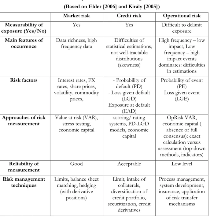
Category of operational risk is worth being compared with the two other main risk categories (market and credit risk). The following table gives a comparison, and flashes all the features of operational risk causing modelling difficulties relatively to market and credit risk:
Table 2 Comparison of main risk categories
(Based on Elder [2006] and Király [2005])
Market risk Credit risk Operational risk Measurability of
exposure (Yes/No) Yes Yes Difficult to delimit
exposure Main features of
occurrence Data richness, high
frequency data Difficulties of statistical estimations,
not well-tractable distributions
(skewness)
High frequency – low impact, Low frequency – high
impact events dominates: difficulties
in estimations Risk factors Interest rates, FX
rates, share prices, volatility, commodity
prices,
- Probability of default (PD) - Loss given default
(LGD) Exposure at default
(EAD)
Probability of event (PE)
Loss given event (LGE) Approaches of risk
measurement
Value at risk (VAR), stress testing, economic capital
scoring/ rating systems, PD-LGD
models, economic capital
OpRisk VAR, economic capital (
absence of full consensus): exact calculation versus assessment (top-down
methods, indicators) Reliability of
measurement Good Acceptable Low level
Risk management
techniques Limits, balance sheet matching, hedging
(with derivative positions)
Limit, intake of collaterals, diversification of
credit portfolio, securitization, credit
derivatives
Process management, system development, insurance, application
of risk transfer mechanisms
The table above presented do not emphasize some other important special feature of operational risk:
Operational risk could be endogenous – external factors could coincide with internal factors causing extremely high severity events, e.g. in case of Barings Bank internal fraudulent activity and external market movements together resulted extremely high loss effect. The other interesting feature: the higher operational risk exposure do not cause obviously higher profit, although in case of market and credit risk, risk exposure and return have positive correlation.
This is why examination of existence and determination of risk appetite or risk tolerance level is an interesting topic.
Before outlining our model framework, it is worth speaking about the operational risk management preparedness of the banking sector: One of the main drivers of systematic operational risk management is regulatory requirement. Following the EU the Capital
Requirements Directive (EU [2006]) is obliged to apply since 1st January 2008. In this new regulatory framework capital should be allocated for operational risk as well, with one of the following methods: simpler, gross income based basic indicator approach (BIA) or the standardised approach (TSA), or more complex Advanced Measurement Approach. Model based approaches are applied now at the most sophisticated institutions, although banks applying simpler methods started to collect loss data in order to ensure the option of more reliable risk assessment later in time.
2.RISK MODELLING FRAMEWORK –STYLISED FACTS
Operational risk could be characterised – as other categories of risk – through frequency of occurrence and severity of loss event. Scaling frequency and severity into two subcategories (low or high) we get 2x2 matrix of risk space. In this case two of the cells will be relevant for us:
High frequency – low severity: events to be easily understood and priced
Low frequency – high severity: events to be prevented and forecasted with important difficulties.
This view is presented at table 3.
Table 3 Main attributes: severity and frequency (Elder [2006])
Low frequency High frequency
High severity
Main challenge for operational risk management
Possible outcome: maybe full disruption
Difficult to forecast, experiences of other sectors (e.g. aviation) could be applied
Not relevant – In case of this risk profile exit from the business could be the optimal solution
Low severity
Not relevant Milder events, could effect strong threats! Events to be easily understood and priced.
Interdependence of events could be existing factor.
Complexity of operational risks (two main focuses mentioned above) makes operational risk modelling complicated. Appropriate input data in terms of quality and quantity is required to provide suitable modelling database.
We could pose the following questions:
1. How the complexity of operational risk could be modelled? Separate modelling of different event categories is necessary for robust estimations?
2. Can we find any holistic approach?
We do not trial to give fully comprehensive answer to these questions in this paper, although one of most important goals of our research going concern is to answer these questions as much as possible in our modelling framework.
There is no modelling approach prescribed by the regulators, we could speak about industry wide best practice methodologies. Based on the operational risk literature we could distinguish two basic types of modelling methods (see e.g. Risk Books [2005], CEBS [2006]):
● loss distribution approach (LDA)
● scenario-based approach (SBA)
Objective of both methods is to determine the necessary economic capital level for operational risk, and to measure risk profile and related exposure accurately.
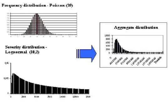
Essentially using LDA methods we determine aggregate distribution (to model loss amount occurring during predetermined period) based on internal loss data history, sometimes supplemented by loss data coming from external loss data sources. Aggregate loss distribution could be derived from frequency and severity distribution through analytic (partly numeric) or Monte-Carlo-simulation based convolution. There are two methods of formal, analytic convolution techniques: recursive methods to be applied in case of discrete distributions (e.g.
Panjer-algorithm); or (Fast) Fourier-Transformation ((F)FT) to applied after discretisation of the distributions given. In practice simulation techniques are applied often, because of the problem could be more easily structured via simulations, although this is a time consuming way, and sensitivity of model could be examined with relatively more difficulties, than analytic techniques (Klugman et al [1997] give good and comprehensive overview of this modelling approach). The following figure summarises and gives an example of convolution methods:
Figure 1 Convolution of frequency and severity distributions
Source: own illustration
The steps of application of LDA approach is the followings: identification of suitable distributions for both of frequency and severity distributions (e.g. Poisson – lognormal model), parameter estimation based on realised loss data, use of goodness of fit tests (GOF tests) and finally model selection and calibration (CEBS [2006]). The regulation (BIS [2004], EU [2006]) in the obligations related to AMA approach defines capital to be held requires a risk measure compatible with 99.9% confidence interval and one year holding period. Note, this is a V@R (value at risk) type calculation based on the analysis of the aggregate distribution. The literature and the practice apply mainly symmetric distributions for frequency modelling (e.g. mainly Poisson–distribution), and mainly asymmetric, fat-tailed distributions for severity distributions
(e.g. lognormal or extreme value distributions (EVT – Extreme Value Theory).
The other important modelling approach, scenario based analysis is also quantitative based method. We determine stress-event scenarios, and through quantitative assessment of these scenarios we calculate the operational risk exposure. As in case of scenario based approaches we examine the structure of operational risk event scenarios, we could say: SBA method is a bottom- up approach, LDA method is a top-down approach in this sense. (CEBS [2006])
Besides LDA and SBA methods, because of difficulties in quantification of operational risk recognised by practitioners, lot of institutions applies more qualitative, so called scorecard techniques (Riskbooks [2005]).
In this paper we would like to look beyond the methods (LDA, SBA) shortly presented above. The methods presented previously are focusing on the modelling of manifested, or manifesting risks in terms of events, but the analysis of latent risk process as interim modelling step generally left out. As our objective to build up a model suitable for support of risk management process, that is why we try to model latent risk factors, and from that we derive the loss event process. Our own model framework and its results are to be presented in the following sections.
3.OWN STOCHATIC PROCESS BASED MODEL –FIRST RESULTS
Stochastic process based modelling is quite often applied for risk phenomena. The basic idea in the risk modelling literature for that type of modelling is factors related to the risk given follow regular process describable in statistical terms.
What could we mean by the term of stochastic process? Concisely we mean by stochastic process that process which describes the changes of X probability variable.
Four main factors or parameters determine a stochastic process (Karlin–Taylor [1985]):
● S state-space (possible value-set of X probability variable, e.g. real numbers);
● T index parameter (That feature of X probability variable, that represent the characteristic of steps in the process, e.g. if T maps the set of non-negative integers that case we speak about discrete process);
● Xt probability variables and the dependence structure among them: initial value should be determined, and based on knowledge of the dependence structure the whole process could be described.
We could apply stochastic process based models for two objectives (see e.g. Cruz [2002]
chapter 7.):
1. Modelling of movement of latent risk factors: in this case break even of a critical level could cause operational risk event attended by some repairing cost or some loss (Cruz [2002]
7.6–7.9 subchapters).
2. Modelling of manifest risk event and amount of loss: In these model-applications the important objective is not the determination of latent risk factors, only ruin process is interesting for the analysing researcher. This approach disposes wide range of actuarial literature; see e.g.
Michaletzky [2001] or Klugman et al. [1997].
The risk modelling literature does not devote too much time for latent risk factor modelling.
Although if we would like to manage the risks, not only measure, latent risk factors do have
essential role, because changes in latent factors could influence the changes in overall risk exposure and risk profile reflected in manifest ruin process. In the remaining part of this paper we present a prototype model for modelling latent risk factors.
We examine the characteristics of operational risk in a simplified model-framework, what we would like to extend to more complex problems in more advanced phase of our research.
Our basic problem is on the following question: how could server disruptions to be modelled?
During the analysis we focus on the risk profile and influencing factors of system failure.
Operational description of the problem:
There is a central server in a bank, which performance fluctuates over time. If performance breaks even a critical level of this factor (two side barrier7), we experience server disruption.
Catastrophe is defined by above mentioned phenomenon, which results a given level of loss.
Another type of problem is that when we have two servers operating. The secondary server is
„hot” back-up server of the first one. In case joint disruption (performance level breaks even the critical level at both servers) we speak about „crash” event, and in this case system could be recovered only with some loss.
Our model assumptions, elements are the following:
1. Performance level process follows mean reversion process: the system reverts back to an equilibrium value, although fluctuation above, and under equilibrium could be occurring.
2. If the process breaks even the lower or upper limit, we speak about catastrophe.
3. After the catastrophe the process gets back to the equilibrium point automatically. The staff repairs the error, and equilibrium state stands back.
4. Loss of catastrophe is commensurable with the measure with the overstepping of performance level limit (linear relationship).
5. Risk process of both servers follows identical stochastic process. The two processes are correlated with each other, while the two servers are identical, and operation of the bank influences both servers8. Due to risk management, or process controlling principles a machine, a process or an employee have a substitute resource, in case of business failure to dispose a substitution resource for having back-up solution.
We could say, some mean reverting type of model could be suitable for above-mentioned assumptions.
Fulfilling these above mentioned requirements we will use the Ornstein-Uhlenbeck process (so called O-U process), widely known in financial mathematics (because of the relative simplicity). This type of process is widely known as Gauss-Markov process as well.
Most known application of OU processes is the Vasicek model used for modelling interest rate movements. (Baxter–Rennie [2002], page 197.). Ornstein-Uhlenbeck process firstly was not applied by financial research, but in neurology to model discharges of neuron, movements of animal, and modelling latent process behind rusting. Generally OU process to be
7 One-side limit (upper or lower limit) could be more reasonable (overloading or underperforming), built in our explanatory research by symmetric barriers we expect to receive well-behaving results. Later in time, during applied research phase we would like to apply asymmetric barriers.
8 Of course, correlation could be decreased by some measures (e.g. separate location), although full removal of correlation is not possible.
applied for latent factor modelling, where manifest process (output, e.g. the data series of events) is known, but the latent factor process is not fully explored ensuring forecasting opportunities.
(e.g. Ditlevsen–Ditlevsen [2006]). Operational risk factors are similar to the factors modelled by OU process in other areas of science: the latent process is not to be observed or could not be observed, only the risk event is explicit.
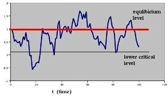
Ornstein–Uhlenbeck-process could be defined by the following differential equation (Based on Finch [2004], sample process on Figure 2.):
dPt = η·(M-Pt) ·dt+σ·dz (1) Concerning notations:
Pt: value of P at time t
η: speed factor of mean reversion,
M: equilibrium rate of P process, performance level process to be reverting to this point, and after a catastrophe the restarting point is hear.
σ: standard deviation parameter
dz: Wiener-process with mean of 0, and standard deviation of 1,
ρ: correlation factor (ρ) is defined in case of joint process representing the alignment feature of the process. (In this case stochastic element of processes is the following: stochastic element of first process is σ·dz, although stochastic element of the second process is
) dy 1
dz
(ρ + −ρ2
⋅
σ , where dy and dz are independent, identical, standard normally distributed Wiener-process.
So the differential equation of the first process is the following: dPt= η·(M-Pt)·dt+σ·dz.
Second differential equation is the following: dPt= η· (M-Pt) ·dt+σ⋅(ρdz+ 1−ρ2dy).
Figure 2 Illustration of Ornstein–Uhlenbeck-process
Source: own illustration, parameters: equilibrium parameter (Μ=1, speed of reversion and standard deviation: η=0.2, σ=0.25)
In mathematics modelling “first time to hit” (FTH) is widely analysed by mathematicians, not only by numeric methods, also by analytic way. (Good reference is: Ditlevsen–Ditlevsen [2006]).
OU process is not limited, that is why unrealistic negative values could be realised as well. In our model framework instead of application of barriers, we apply a standing back step to the equilibrium value of the process.
3.1. Model results
Hereinafter we would like to present the basic model results: we analyse the risk process, and demonstrate the frequency and severity features related to the catastrophe events. Firstly we examine the single process, later the dual process. Simulation method is to be applied, with realisations of 10 samples, 10.000 unit long period. When we apply large number of samples, we apply 10.000 samples with 10.000 unit long period sample by sample. We model OU process based on formula (1) mentioned above. For purposes of analysis, statistical calculations we used Borland Delphi 5.0 and SPSS 14.0 for Windows software. On the figures parameter settings are indicated, in case of multiple runs we refer on it in the text. Current phase of our research is more or less explorative, that is why now we would like to explore some basic trends supporting to structure robust and stable model later in time.
3.1.1. Analysis of single process
Empirical analysis shows us that the core process (OU process) values could characterised by normal distribution (as we have expected from the features of OU process).
Figure 3 Characterisation of basic OU process with given parameterisation
Source: own calculation (process values, histogram of output values and parameterisation)
Based on the application of Kolgomorov–Smirnov-statistics (value is 0.615) we could not reject that hypothesis that values of the process follows normal distribution. Certainly in case of limit tightening the process values would follow truncated normal distribution.
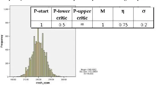
First of all it is worth examining the frequency distribution of catastrophes. In contrast of the process illustrated on the figure 3, on the following figure we show the frequency features of a process with asymmetric limitations, only lower limit:
Figure 4 Frequency distribution of catastrophe of a process with a given parameterisation
Source: own calculations
In operational risk literature frequently assumed that occurrence of operational risk events could be characterised by Poisson process. (We have referred on this in chapter 2). As the figure 4 shows in our model frequency could be characterised by symmetry. It is worth to test, with what kind of parameterisations Poisson like behaviour hypothesis could not be rejected. (E.g. Bee [2006]) We have tested with three types of limitation features (broader two-sided, tighter two- sided, tightened lower and upper unconstrained limit-parameterisation) goodness of fit for
P-start P-lower critic
P-upper critic
M η σ
1 0.25 2 1 0.75 0.25
Poisson-distribution fitting, ceteris paribus to the parameterisation showed on figure 4:
Table 4 Goodness of Poisson distribution fitting by different limitations parameters
P-start P-lower
critic K-S Z Sigma 0.25 2 2.129 0
0.5 1.5 0.406 0.996
0.5 ∞ 0.794 0.554
Kolgomorov-Smirnov Z statistics presented on Table 4 shows us, that in case of tightened two-sided limitation and by one-sided limitation Poisson characteristics could not be rejected. In case of broader limit Poisson feature could not be accepted.
As mentioned previously, in probability theory literature dealing with OU type processes one of most examined topic is another aspect of frequency, the so called “first time to hit”
(FTH), the timing of the first break-even point. Ditlevsen–Ditlevsen [2006] presents, that probability distribution of „first time to hit” could be described in analytic way in a very complicated way. In case of special parameterisation FTH follows Poisson distribution (when equilibrium value and critical value have long distance from each other), while in other cases it some sums of gamma distributions.
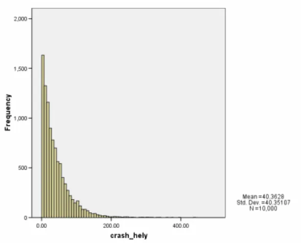
Similarly to frequency examination we have examined FTH distribution for different parameterisations. The following figure shows one the example of this:
Figure 5 Distribution of first time to hit by tightened limit parameterisations (critical
values: 0.5 and 1.5)
Source: own calculations
We could observe skewed distribution of „first time to hit” on Figure 5. Poisson or gamma distribution fitting is not adequate, although based on theoretical works these distributions could be applied. However we experienced good fit of Poisson distribution for catastrophe frequency, and it is known the distribution of time between events follows exponential distribution, so we can have hypothesis on empirical goodness of fit for exponential distribution:
Table 5 Goodness of fit test applied for the fit of distribution of „first time to hit” and
exponential distribution P-start P-lower
critic K-S Z Sigma
0.25 2 2.470 0.000
0.5 1.5 0.736 0.650
0.5 ∞ 4.907 0.000
Source: own illustration
As on the table above presented, goodness of fit tests (e.g. K-S Z-score) signs, in case of tightened two-sided limitations the exponential could not be rejected, in case of other two parameterisations exponential fit is not good. That is why distribution of „first time to hit”
should be analysed analytically with more effort.
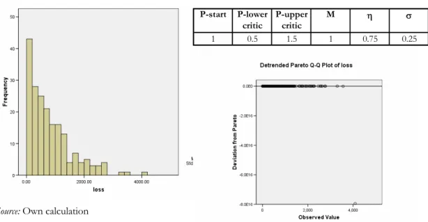
We have examined the severity distribution as well. We applied the following regularity for determination of the amount of loss: value of loss is absolute value excess above upper limit or under lower limit multiplied by unit of 10 000. This is a linear relationship, could be reasoned by economic idea. (E.g. There is a catastrophe at level of 0.4 in case of lower level 0.5, in that case the excess value under lower level is 0.1, and that is why the loss is 1000 unit). Applying this assumption we received well behaving severity distributions fulfilling the preliminary expectations of asymmetry and fat-tailed property. We present below an empirical distribution in case of given parameterisation, and goodness of fit with Pareto distribution fairly acceptable as showed by Q-Q plot:
Figure 6 Severity distribution and its fit to Pareto distribution
Source: Own calculation
P-start P-lower critic
P-upper critic
M η σ
1 0.5 1.5 1 0.75 0.25
Pareto distribution is a typical left-skewed, fat-tailed distribution reflecting well the high frequency of low impact events, and low frequency of high impact events. The Pareto distribution type, applied originally by Vilfredo Pareto in order to characterise the distribution of wealth among people, is often used in actuarial literature.
The formula of Pareto probability density function is the following:
) 1
x ) ( x (
f α+
α
θ +
θ
⋅
= α (2),
where α is the so called location parameter, while θ is the shape parameter. (Cruz [2002]
page 53.; Michaletzky [2001] page 156.)
As we could see, the observed patterns of frequency and severity could fulfil the preliminary assumptions applied for operational risk: symmetric frequency distribution, skew, fat-tailed severity distribution.
3.1.2. Examination of dual process
Besides single process we have examined the features of dual process as well.
In case of dual disruption of originally operating system and back-up system, we could speak about joint catastrophe, about crash. As a story they say: there was bank during 11/09 WTC-catastrophe, which had hot system in one of the twin towers, while the hot back-up system operated in the other tower of WTC. After the collapse of both towers, the institution was forced to continue its operation after recovery from data savings.
In case of dual process we have examined the same features as in case of single process:
frequency of catastrophe event, first time to hit, severity distribution, although we focus on joint catastrophe events (crashes). In case of first sample both processes have same parameter settings, correlation coefficient is built in via stochastic element.
It is a trivial expectation that in case of broader limitations we experience fewer crashes, although in case of tightened limitations we experience more crashes and as illustrated below symmetric distribution fit for frequency could not be rejected.
Figure 7 Frequency distribution of joint catastrophes („crashes”) by broader limitations
and tightened limitations
Source: own calculation
Besides tightened limitations (0.5-1.5) fit for Poisson distribution could not be rejected based on Kolgomorov–Smirnov Z-test statistics (value: 0.455).
„First time to hit” distribution could not be identified based on visual inspection. As Figure 8 illustrates only few number of joint catastrophe occurred in case of broader limitations, at the dominant part of samples there was no crash occurred (8000 samples from 10 000 samples).
In case of filtering for that sample which contains crash event (right side of Figure 8), we get a visually unidentifiable distribution.
Figure 8
„First time to hit” distribution for crash events
Source: own calculations
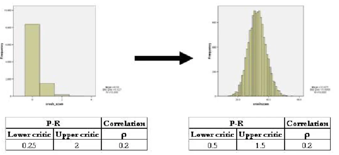
The other important topic is to examine the severity distribution for catastrophes. We apply the same loss measure as in case of single process: value of loss is absolute value excess above upper limit or under lower limit multiplied by unit of 10 000. In uncorrelated case of dual process we receive acceptable fit for Pareto distribution, as illustrated on the figure bellow:
Figure 9 Severity distribution related to dual process in case of given parameterisation
Source: own calculations
Wilcoxon test run in SPSS (comparison of empirical data series and Pareto random numbers) shows us that deviation from Pareto distribution is not significant (value of two sided sigma is 0.195).
Dependency on correlation could sign up with strong emphasis in case of severity that is why optimalisation of correlation has great importance. We tested this phenomenon the process showed on Figure 9.: with correlation of zero and medium sized correlation (0.5) Based on calculation of the distribution moments we have experienced that in parallel with increase in correlation mean, skewness, kurtosis and variance increased as well:
Table 6 Moments of severity distributions for dual process by two correlation value Correlation Mean Variance Skewness Kurtosis
0 693.91 663.04 1.73 3.97
0.5 765.69 734.34 2.05 6.21
Comment: parameter settings except for correlation is the same as it was by Figure 9
This result could be dealt as triviality, but based on it the relationship between correlation and severity should be examined in more details.
3.1.3. Parameter sensibility of the catastrophe frequency
In this section we analyze the sensibility of our model. We analyze how the slight changes in reversion speed (η) and correlation (ρ) affect the crash-frequency. We consider this also as the partial verification of our simulation method, while the introduced results confirm our previous hypotheses.
The increase of the reversion speed parameter definitely decreases the expected value of the number of crashes at both the single and the dual process models.
Figure 10
-1.0 0.0 1.0 2.0 3.0 4.0 5.0 6.0
0.00 0.20 0.40 0.60 0.80 1.00
R - η
number of crashes
Mean
Mean + St. Dev.
Mean - St. Dev.
Single process:
Dual process:
0 100 200 300 400 500 600
0.01 0.11
0.21 0.31 0.41
0.51 0.60
0.70 0.80
0.90 η
Number of catastrophes
Mean + St. Dev.
Mean - St. Dev.
Mean
P-start P-lower critic P-upper critic M σ
1 0.5 1.5 1 0.25
Correlation P R
Start Lower critic Upper critic M σ ρ η η
1 0.25 2 1 0.25 0.2 0.51 variable
P-R
The increase of the reversion speed decreases the expected value of the crashes (joint catastrophe analysed at the dual model).
The increase of correlation parameter is the following: the stronger the correlation between the two processes, the more often the estimated value of the dual crash frequency. At the following figure we demonstrate a bounded series of realization at different correlation parameters.
Figure 11
0 50 100 150 200 250 300 350 400
0.0 0.1 0.2 0.3 0.4 0.5 0.6 0.7 0.8 0.9
ρ
number of catastrophes
Mean
Mean + St. Dev.
Mean - St. Dev.
Correlation Start Lower critic Upper critic M η σ ρ
1 0.5 1.5 1 0.75 0.25 variable
P-R
The increase of the correlation increases the expected value of the joint catastrophes (crashes)
Naturally, during our further researches to be conducted later it is necessary to analyze more precisely the sensitivity of the parameters. Beside the speed of mean reversion and the correlation parameter, the other input parameters should be analyzed later.
3.2. Forecasting the operational risk
One of the important objectives of the risk analysis is risk profile based forecasting. Analyzing the historical database of the past events, we prepare to the emergence of future risks. As we presented in the second part of this paper, the key-point of the operational risk analysis, is the modelling of the low frequency high impact (LFHI) events. In this case the risk forecasting can raise difficulties. We distinguish two basic methods to forecast risk events (catastrophes): 9
1. Based on the past occurrence of the risk events: We analyze the frequency and the impact (severity) of the catastrophe events. 10 We suppose, that the estimated risk parameters are suitable for forecasting. (The terminology for same methodology of credit default estimation is the “k/n” method.) The essence of this approach is that we use a small sample for estimation, and we use naïve forecasting, as we suppose parameter stability.
(The future parameters and the past parameters are supposed to be the same: future fully reflects past)
9 Naturally, we can extrapolate historical data in many different ways (e.g.: moving average, smoothing techniques, etc.), but here we examine two basic methods.
10 External loss-databases can have a high impact on the processing of the previous chatastrophe events. (E.g.:
HunOR Hungarian Operational Risk Database).
2. Based on the exploration of the latent risk process: We analyze the previous risk events, and reproduce the latent risk process. Based on computer simulation methods, we can give forecasting. We run the latent risk process based on our flexible modelling assumptions and parameters, then we generate the forecasting of the future risk (events and factors) based on the simulation results. We might simulate many replication of the latent risk process (fix length, hit analysis), or simulate only one very long period (steady-state simulation). 11
Note, that the real target of our analysis is not the forecasting, but – assuming the risk profile stability (in time) – the best estimation, in classical terms.
When comparing the different methods our starting-points of the analyses were the following: 12 1. We are acquainted with the single run of the latent risk process (for 100, 250 and 1000 unit length periods). The concrete database is a single realization of a previously defined OU-process.
2. We suppose the stability of the latent OU-process, and that will go on with the same parameters in the future, as we supposed this at the small-sample estimation, too.
Next, we continue the analyses of the single and dual processes separately.
3.2.1. Risk forecasting by simulated processes
In this section, we analyzed two different parameter-settings:
1. Strict catastrophe criterion (broader tolerance level - low catastrophe event frequency): The lower limit value of crash is 0, the higher limit value is 2. The starting value, and the equilibrium state of the process is 1. The reversion speed parameter value is (η) 1, and the deviation (σ) is 0.25.
2. Wider catastrophe criterion (tightened tolerance level - higher catastrophe event frequency):
The lower limit value of crash is 0.4, the higher limit value is 1.6 (narrower, symmetric range). The starting value, and the equilibrium state of the process is 1, as before. The reversion speed is (η) 0.75 (thus the process can return to equilibrium slower), and the deviation (σ) is 0.25.13
In the following table we compare the different crash frequencies of the parameter-settings at different sample size and length period:
11 Simulation terminology calls „batch mean” method, when we split the steady state simulation to smaller periods (batches).
12 Naturally, we must loose the restrictions as much as possible during the further researches.
13 Parameter-settings are arbitrary. The main purpose was to present different situations.
Table 7 Crash frequency simulation for the different parameter-settings
1. Strict catastrophe criterion (broader range of tolerance)
Number of
simulation Sample size
(number of runs) Length of period
(T) Total number of crashes during the period
Estimated crash probability
1 1 100 0
-
2 1 250 0
-
3 1 1000 0
-
4 10000 100 56
0.006%
5 10000 250 175
0.007%
6 10000 1000 629
0.006%
7 1 10000 1
0.010%
8 1 100000 12
0.012%
2. Wider catastrophe criterion (tightened range of tolerance)
Number of
simulation Sample size
(number of runs) Length of period
(T) Total number of crashes during the period
Estimated crash probability
1 1 100 2
2.000%
2 1 250 4
1.600%
3 1 1000 18
1.800%
4 10000 100 19234
1.923%
5 10000 250 48163
1.927%
6 10000 1000 192031
1.920%
7 1 10000 190
1.900%
8 1 100000 1915
1.915%
Source: own simulation results
Small sample estimation of crash frequency at the first parameter-setting cannot be reliable. In this case, no catastrophe event occurred, thus we would definitely underestimate the risk frequency.
Using simulation (large size sample) we get more conservative results. That means that without simulation, we can usually underestimate our risks. The statistical applicability of simulation methods is based on a probability theory statement. The essence of the Glivenko-Cantelli statement is the following: the empirical distribution function of the observed simulation outputs,
tends to the real, latent distribution function, with the probability of 1.
Formally: P(supt | Fn*(t) - F(t) | → 0 ) = 1, where * notes the empirical distribution, F(t) is the latent distribution function of the t random variable, Fn*(t) is the empirical distribution function of t random variable at n realization of the simulation, and P(x) is the probability of the x event.
However the second parameter-setting, where the catastrophe events are more often, the small sample observation would overestimate the market risk.
Taking a longer period (T = 100 000 unit) we observed how the error rate (number of crashes divided by the passed period) changes in the function of the expansion of the simulation period.
We can realize an un-hoped convergence of the error rate, as we examine the strict risk definition. At the beginning of the simulation run, the deviation is larger, but later the convergence of the result is trivial. (See Figure 12)
Figure 12 Fluctuation of catastrophe ratio (tolerance level: 0-2)
-0.02%
0.00%
0.02%
0.04%
0.06%
0.08%
0.10%
0.12%
0.14%
0.16%
0 10,000 20,000 30,000 40,000 50,000 60,000 70,000 80,000 90,000 100,000 Parameterisation:
P(lower critic) - 0 - P(upper critic) - 2 P (start) - 1 Equlibrium value - 1 η= 1; σ= 0.25
Source: Error- (catastrophe-) rate in the function of the sample size at wider catastrophe criterion (simulation results of the authors)
This convergence path is more evident and faster at the stricter catastrophe criterion parameter- setting (see Figure 13)
Figure 13 Fluctuation of catastrophe ratio (tolerance level: 0.4 - 1.6)
0.000 0.005 0.010 0.015 0.020 0.025
0 10,000 20,000 30,000 40,000 50,000 60,000 70,000 80,000 90,000 100,000
Parameterisation:
P(lower) - 0.4 - P(upper) - 1.6 P (start) - 1 Equlibrium value - 1 η= 0.75; σ= 0.25
Source: Error- (catastrophe-) rate in the function of the sample size at stricter catastrophe criterion (simulation results of the authors)
The forecasting of the loss amount at the single crash process is also an interesting problem.
Suppose, that loss amount has still a positive correlation with the exit distances from the tolerance ranges. We introduce the most important characteristics (moments) of the impact distribution function at Table 8:
Table 8 Simulation results of the impact (seriousness) forecasts for the single process, at the two
parameter-settings 1. Strict catastrophe criterion (broader range of tolerance)
Number of
simulation Sample size (number of runs)
Length of
period (T) Average Standard
deviation Skewness Kurtosis
1 1 100 No
catastrophe No catastrophe No catastrophe No catastrophe
2 1 250 No
catastrophe No catastrophe No catastrophe No catastrophe
3 1 1000 No
catastrophe No catastrophe No catastrophe No catastrophe
4 10000 100 479.34 462.60 2.17 5.91
5 10000 250 496.77 538.41 2.56 8.75
6 10000 1000 553.02 507.58 1.52 3.05
7 1 10000 111.15 0 (1
catastrophe) 0 (1 catastrophe) 0 (1 catastrophe)
8 1 100000 642.29 616.82 0.67 –0.74
2. Wider catastrophe criterion (tightened range of tolerance)
Number of
simulation Sample size (number of
runs)
Length of
period (T) Average Standard
deviation Skewness Kurtosis
1 1 100 1019.16 114.67 Number of joint
catastrophes < 3
Number of joint catastrophes < 4
2 1 250 664.61 417.10 0.62 1.19
3 1 1000 1207.82 1137.91 1.60 2.84
4 10000 100 865.24 806.35 1.60 3.21
5 10000 250 867.48 799.88 1.59 3.35
6 10000 1000 877.29 784.18 1.52 2.87
7 1 10000 819.65 766.29 1.37 1.35
8 1 100000 849.85 790.31 1.74 4.55
Source: own simulation results
The analysis of impact (seriousness) is similar to the frequency results. At low frequency catastrophes we might have an underestimation from small sample, and at high frequency catastrophes we might have an overestimation (derived form the moments). However, comparing those simulations, where we analyzed 10 000 small sample, we see some increase in the estimated risk.
3.2.2. Risk forecasting for dual process
In this section we analyze the characteristics of the joint crash processes. Joint catastrophes (“crash”) frequency forecasting, from small sample rise difficulties.
We applied two different parameter settings in this case, too:
We applied two different parameter settings in this case, too:
1. Two strongly correlated processes: The lower limit value of crash is 0.1, the higher limit value is 1.9. The starting value, and the equilibrium state of the process is 1. The reversion speed parameter value is (η) 0.75, the deviation (σ) is 0.25. The correlation (ρ) is 0.8.
2. Two weakly correlated processes: The lower limit value of crash is 0.1, the higher limit value is 1.9. The starting value, and the equilibrium state of the process is 1. The reversion speed parameter value is (η) 0.75, the deviation (σ) is 0.25. The correlation (ρ) is 0.1.
At the weakly correlated processes the frequency of crashes is rare, just as we supposed. The results are summarized in the following table.
Table 9 Simulation results of forecasting for the dual processes at two different parameter-
settings
1. Two strongly correlated processes (correlation = 0.8)
Number of simulation
Sample size (number of runs)
Length of period (T)
Total number of joint
catastrophes (crashes) during the period
Estimated joint catastrophe (crash) probability
1 1 100 0
-
2 1 250 0
-
3 1 1000 1
0.1000%
4 10000 100 92
0.0092%
5 10000 250 242
0.0097%
6 10000 1000 1066
0.0107%
7 1 10000 1
0.0100%
8 1 100000 11
0.0110%
2. Two weakly correlated processes (correlation=0.1)
Number of simulation
Sample size (number of runs)
Length of period (T)
Total number of joint
catastrophes (crashes) during the period
Estimated joint catastrophe (crash) probability
1 1 100 0
-
2 1 250 0
-
3 1 1000 0
-
4 10000 100 0
-
5 10000 250 3
0.0001%
6 10000 1000 8
0.0001%
Number of simulation
Sample size (number of runs)
Length of period (T)
Total number of joint
catastrophes (crashes) during the period
Estimated joint catastrophe (crash) probability
7 1 10000 0
-
8 1 100000 0
- Source: Own simulation results of the authors
We analyzed the probability of single and joint catastrophes, too. When the correlation was stronger, we observed higher deviation and longer convergence of the error rate (see Figure 14).
At weaker correlation, we observed more obvious and faster convergence (see Figure 15).
Figure 14.
Catastrophe ration (tolerance level: 0.1-1.9)
0.00%
0.05%
0.10%
0.15%
0.20%
0.25%
0.30%
0.35%
0.40%
0 10,000 20,000 30,000 40,000 50,000 60,000 70,000 80,000 90,000 100,000
Catastrophe ratio Joint catastrophe (crash) ratio Parameterisation:
P(lower) - 0.1 - P(upper) - 1.9 P (start) - 1 equilibrium value - 1 η= 0.75; σ= 0.25
correlation = 0.8
Source: Error- (catastrophe-) rate in the function of the sample size, for joint catastrophes (crash), at stronger correlation (own simulation results)
Figure 15 Catastrophe ration (tolerance level: 0.1-1.9)
0.00%
0.05%
0.10%
0.15%
0.20%
0.25%
0.30%
0.35%
0.40%
0 10,000 20,000 30,000 40,000 50,000 60,000 70,000 80,000 90,000 100,000
Catastrophe ratio Joint catastrophe (crash) ratio Parameterisation:
P(lower) - 0.1 - P(upper) - 1.9 P (start) - 1 equilibrium value - 1 h= 0.75; s= 0.25
correlation = 0.1
Source: Error- (catastrophe-) rate in the function of the sample size, for joint catastrophes, at weaker correlation (own simulation results)
As we can see, the joint catastrophe (“crash”) rate is stable 0%, thus at weaker correlation, it is useful to select a larger sample.
CONCLUSION, TOPICS FOR FURTHER RESEARCHES
In this paper we presented results of our exploratory research. We could conclude, that our model results accords the assumptions provided by operational risk literature. Our simplified model presented in this paper is good basis for further modelling of operational risk events and influencing factors. Empirical frequency distribution could be fitted quite well onto Poisson- distribution; while severity distribution could be fitted by Pareto distribution14. Distribution of
„first hitting time” playing a key role in related mathematical literature shows us great complexity in our empirical research. We have examined the model-based forecasting opportunities, and we experienced small sample based method could result biased estimations (over- or underestimation).
We need to study in more deepness the theoretical mathematics literature related to analytical analysis of OU processes for comparison of empirical and theoretical frequency, severity and FTH distributions. Further study of parameter sensitiveness and aggregate (loss amount / prespecified period) distribution in order of capital calculations would be also a good topic of further research. Our objective for practical implementability is the estimation of process of latent factors based on the realised event points, based on some assumptions, and based on the latent factor process estimation we would like to forecast and fit our results onto concrete risk categories (e.g. system failures, ATM disruptions, frauds etc.). These types of models of course could be valid, if model results accord to the real banking experiences.
14 Besides Pareto distribution lognormal or Weibull distributions are frequently fitted on severity distribution.
We need to apply goodness of fit tests (GOF-tests) for identification of appropriate type of distribution.
REFERENCES
BAXTER,M.–RENNIE,A. [2002]: Pénzügyi kalkulus, Typotex, Budapest
BEE,MARCO [2006]: Estimating the parameters in the Loss Distribution Approach: How can we deal truncated data in „The advanced measurement approach to operational risk”, Risk books, London
BIS [2004]: International Convergence of Capital Measurement and Capital Standards: a Revised Framework, 26th June 2004., http://www.bis.org/publ/bcbs107.pdf (2nd January 2007.) CEBS [2006]: GL10 – Guidelines on the implementation, validation and assessment of Advanced
Measurement (AMA) and Internal Ratings Based (IRB) Approaches, www.c-ebs.org CRUZ,MARCELO [2002]: Modelling, measuring and hedging operational risk, John Wiley & Sons,
Chichester
DITLEVSEN,SUSANNE–DITLEVSEN,OVE [2006]: Parameter estimation from observation of first passage times of the Ornstein-Uhlenbeck Process and the Feller process, Conference paper: Fifth Computational Stochastics Mechanics Conference, Rhodos, June 2006
ELDER, JAMES [2006]: Using scenario analysis to estimate Operational Risk Capital, London, Operational Risk Europe Conference
European Union (EU) [2006]: Directive 2006/48/EC of the European Parliament and of the Council of 14 June 2006 relating to the taking up and pursuit of the business of credit institutions (recast) (Text with EEA relevance)
FINCH, STEVEN [2004]: Ornstein Uhlenbeck process, elérés: http://algo.inria.fr/csolve/ou.pdf (26th October 2007.)
JORION,PHILIP [1999]: A kockáztatott érték, Panem Könyvkiadó, Budapest
KARLIN,S.–TAYLOR,M.H. [1985]: Sztochasztikus folyamatok, Gondolat Kiadó, Budapest
KIRÁLY, JÚLIA [2005]: Kockáztatottérték-számítások, előadássorozat, Budapesti Corvinus Egyetem
KLUGMAN, S.– PANJER, H.–WILMOT, G. [1997]: Loss Models, Wiley Series in Probability and Statistics, Wiley, New York
MICHALETZKY,GYÖRGY [2001]: Kockázati folyamatok, ELTE Eötvös kiadó, Budapest
ORX [2007]: ORX reporting standards, internetes elérhetőség:
http://www.orx.org/lib/dam/1000/ORRS-Feb-07.pdf (26th July 2007.)
PSZÁF [2005]: Az új tőkemegfelelési szabályozással kapcsolatos felkészülésre vonatkozó kérdőívre beérkezett válaszok feldolgozása, Budapest, www.pszaf.hu (Hungarian Financial Supervisory Authority)
Risk Books [2005]: Basel II handbook for practioners, Risk Books, London
VEERARAGHAVAN, M. [2004]: Stochastic processes, előadásjegyzet, http://www.ece.virginia.edu/~mv/edu/715/lectures/SP.pdf (26th October 2007.)
![Table 1 Operational risk vs. „other risk (based on Cruz [2002b])](https://thumb-eu.123doks.com/thumbv2/9dokorg/947422.54800/5.892.95.803.177.445/table-operational-risk-vs-risk-based-cruz-b.webp)
![Table 3 Main attributes: severity and frequency (Elder [2006])](https://thumb-eu.123doks.com/thumbv2/9dokorg/947422.54800/7.892.201.713.527.881/table-main-attributes-severity-frequency-elder.webp)