Composite Higgs models on the lattice
Hungarian Academy of Sciences doctoral thesis
Daniel Nogradi
Eotvos Lorand University
Institute of Physics
Department of Theoretical Physics
2017
Acknowledgments
I would like to thank my collaborators throughout the years with whom I was working on the topics contained in this thesis. It was a pleasure working closely together with Julius Kuti, Zoltan Fodor and Kieran Holland on various aspects of composite Higgs dynamics in the past 10 years and I have learned a lot from all of them. We were joined by several researchers at various stages of our work, Chris Schroeder, Ricky Wong and Santanu Mondal, all of whom were always ready to discuss physics whether related to our work or not.
I also would like to thank Sandor Katz, Szabolcs Borsanyi, Kalman Szabo, Chris- tian Hoelbling, Stefan Krieg, Balint Toth, Norbert Trombitas, Stephan Durr, Simon Mages, Thomas Lippert and Attila Pasztor with whom I have collaborated on the topic of QCD thermodynamics on the lattice. This collaboration also shaped my thinking about strongly interacting gauge theories in general and hence was extremely helpful for our work on composite Higgs dynamics presented in this thesis.
Contents
1 Introduction and conclusion 5
2 Review of the field, techniques and methods 9
2.1 Introduction . . . 9
2.2 Strong dynamics and a light scalar . . . 11
2.3 Gauge theories inside and outside the conformal window . . . 12
2.3.1 Infinite volume, zero mass . . . 12
2.3.2 Finite volume, non-zero mass . . . 14
2.4 Mass spectrum as a probe for IR-conformality . . . 16
2.4.1 Finite volume effects . . . 16
2.4.2 Finite lattice spacing effects . . . 17
2.4.3 Low lying scalar and chiral perturbation theory . . . 17
2.4.4 Selected lattice results . . . 18
2.5 Running coupling as a probe for IR-conformality . . . 19
2.5.1 Static potential . . . 20
2.5.2 Vector current . . . 21
2.5.3 Schr¨odinger functional (SF) coupling . . . 22
2.5.4 Gradient flow (GF) coupling . . . 23
2.5.5 Nucleon mass . . . 25
2.5.6 Continuum limit of finite-volume couplings . . . 25
2.5.7 Anomalous dimension of ¯ψψ. . . 27
2.6 Outlook . . . 27
3 A toy model of confining, walking and conformal gauge theories 28 3.1 Introduction . . . 28
3.2 O(3) sigma model with aθ-term . . . 30
3.3 Numerical simulation . . . 31
3.4 Summary and conclusion . . . 32
4 Sextet composite Higgs model 35 4.1 Introduction . . . 35
4.2 Electroweak multiplet structure, gauge anomalies, and baryons . . . 36
4.2.1 Electroweak multiplet structure . . . 36
4.2.2 Anomaly conditions . . . 37
4.2.3 Sextet baryons and the Early Universe . . . 37
4.2.4 Ongoing lattice work on sextet baryons . . . 37
4.3 Mass-deformed chiral perturbation theory and the chiral condensate . . 38
4.3.1 Taste breaking cutoff effects in the staggered pion spectrum . . . 39
4.3.2 Fundamental parameters from rooted staggered chiral perturba-
tion theory (p-regime) . . . 39
4.3.3 Epsilon-regime, RMT, and mixed action in the valence sector . . 42
4.4 The light 0++ scalar and the resonance spectrum . . . 44
4.4.1 The light scalar state . . . 44
4.4.2 The emerging resonance spectroscopy . . . 45
4.5 Running coupling . . . 46
4.5.1 The gradient flow running coupling scheme . . . 46
4.5.2 Rooted staggered formulation . . . 47
4.5.3 Review of rooting in infinite volume . . . 48
4.5.4 Rooting in finite physical volume at zero bare mass . . . 49
4.5.5 The bridge to large volume physics and simulations at finite cutoffaf . . . 51
4.5.6 Numerical simulation . . . 51
4.5.7 Continuum extrapolation . . . 55
4.5.8 Systematic error estimate . . . 56
4.5.9 Final results . . . 59
5 Many fundamental flavors 61 5.1 Chiral symmetry breaking below the conformal window . . . 62
5.1.1 Staggered chiral perturbation theory . . . 62
5.1.2 Finite volume analysis in the p-regime . . . 63
5.1.3 δ-regime and-regime . . . 64
5.2 Simulations results in the p-regime . . . 65
5.3 Epsilon regime, Dirac spectrum and RMT . . . 67
5.4 Inside the conformal window . . . 70
5.4.1 Conformal dynamics in finite volume . . . 70
5.4.2 Running coupling and beta function . . . 71
5.5 Gradient flow running couplingNf = 4 . . . 74
5.5.1 Introduction and summary . . . 74
5.5.2 Small volume expansion . . . 75
5.5.3 Yang-Mills gradient flow onT4 . . . 78
5.5.4 Running coupling . . . 80
5.5.5 Numerical results . . . 81
5.6 Gradient flow running couplingNf = 8 . . . 84
5.6.1 Numerical simulation . . . 85
5.6.2 Continuum extrapolation . . . 87
5.6.3 Systematic error . . . 87
5.6.4 Final results . . . 91
5.7 Gradient flow running couplingNf = 12 . . . 94
5.7.1 Introduction and motivation . . . 94
5.7.2 Lattice implementation of the stepβ-function . . . 95
5.7.3 Simulation setup . . . 96
5.7.4 Continuum extrapolation . . . 97
5.7.5 Conclusions . . . 97
5.8 Running coupling summary . . . 100
Chapter 1
Introduction and conclusion
The 2012 discovery of a relatively light Higgs boson with a mass of approximately 125 GeV at the Large Hadron Collider in CERN was a major milestone in our un- derstanding of the Standard Model of particle physics and the electro-weak sector in particular [1,2]. The discovery provided the last missing piece of the Standard Model which successfully describes the visible Universe with astonishing precision. The high precision achieved is only possible as a result of very precise theoretical calculations based on the Standard Model and very precise measurements at our accelerators, per- formed over the course of the past 40 years.
Even though the discovery crowned the Standand Model as the most precise and most detailed description of the elementary particles and their interactions, there are a number of shortcomings that are nevertheless present. These shortcomings are not new but gained further prominence by the precise knowledge of the Higgs mass, which was a free parameter prior to 2012. One of these shortcomings is inherent to the Standard Model itself and is usually referred to as the hierarchy problem or fine tuning problem.
More specifically, the 125 GeV Higgs mass in the Standard Model is a result of an enormous cancellation between two terms with typical sizes 1019 GeV but opposite signs. Technically, this cancellation is necessary to account for the 125 GeV mass because the Higgs particle is described by an elementary spin-0 scalar field whose mass is not protected by any symmetries. The Planck scale 1019 GeV comes about as the highest possible scale where the Standard Model can still be valid, beyond that quantum graviational effects certainly kick in. This large hierarchy of scales or the necessary associated fine tuning is highly unnatural and certainly not something we have seen in other phenomena in Nature. The only way to resolve this apparent paradox is to introduce new hitherto unobserved particle sectors well below the Planck scale, i.e. new physics beyond the Standard Model.
The other set of shortcomings of the Standard Model come from cosmological observations and also call for new physics. It is well established by now that only about 5% of the Universe is visible i.e. the Standard Model only applies to this small fraction.
The remaining 95% consists of two parts, about 27% dark matter and 68% dark energy, the latter of which may be accounted for by a cosmological constant. The dark matter sector can not be explained by any particle content already present in the Standard Model (such as neutral hadrons or neutrinos) as direct detection experiments [3–6]
would have seen it already. The only concievable way to have a description for this approximately 27% of the Universe is to introduce new particles and new interactions to the Standard Model. Any new model of dark matter will be tested by experimental
results from dedicated detectors (XENON [3], LUX [4], CDMS [5], among others), the Large Hadron Collider and by cosmological observations.
There are (infinitely) many ways in which the Standard Model can be extended to account for dark matter or any new physics which solves the hierarchy problem.
Present and past experimental results set stringent constraints of course, but the pos- sibilities are still vast. The only way forward seems to be reasonable guidelines or general principles which proved useful in particle physics before and are sufficiently well-motivated. One of these guidelines that I find most persuasive is the observation that the mass in the well-understood 5% of the Universe is the result of strong inter- actions. Even though according to the Standard Model the Higgs particle provides masses to the leptons and quarks (along with theW andZ bosons) the vast majority of the observed mass of stable particles in the visible Universe is originating from the strongly interacting dynamics of Quantum Chromodynamics (QCD) [7]. In QCD the elementary building blocks, quarks and gluons, are not observed directly as stable par- ticles but rather only their composits, baryons or potentially glueballs. Incidentally, QCD is free from any fine tuning problems and is truely a fundamental theory. Hence it is natural to assume that viable theories beyond the Standard Model will be based on strongly interacting models and the observable particles will be composits of more elementary building blocks. This is especially likely for dark matter since about the only aspect we are certain about it is that it contributes a large fraction of the total mass of the Universe. This approach, if applied to the Higgs sector of the Standard Model, also leads to the possibility that the Higgs boson is a composite particle itself and hence the fine tuning problem is averted for the lack of an elementary spin-0 scalar particle.
A key feature of QCD is that it is an asymptotically free non-abelian gauge theory.
Asymptotic freedom guarantees the lack of a fine tuning problem, although the more lax requirement of asymptotic safety would also be sufficient. The very nature of non-abelian gauge theories is that they are generically strongly interacting and hence are notoriously difficult to study quantitatively. The experience from QCD and more recently strongly interacting extensions of the Standard Model nevertheless suggests that numerical simulations will be able to allow for robust and quantitative conclusions regarding specific models for physics beyond the Standard Model.
Our class of extensions replaces the essentially weakly coupled Higgs sector by strong coupling dynamics, the idea being guided by analogies from QCD [8,9]. Electro- weak symmetry breaking in the Standard Model is then the analog of spontaneous chiral symmetry breaking in QCD and hypothetical new particles called technifermions and technigluons are analogs of fermions and gluons in QCD. This analogy is appealing because symmetry breaking becomes a dynamical phenomenon and the fine tuning problem is solved. Models based on this analogy are often called Strong Dynamics models and will of course only be viable if all constraints given by the known and confirmed sectors of the Standard Model are fulfilled.
One such constraint is that the coupling constant of the model should not change much over a considerable energy range and should be large, i.e. the coupling constant should walk. The reason for walking is that without it a tension exists between the observed smallness of Flavor Changing Neutral Currents and the fermion masses [10, 11]. Walking behavior is expected to occur for theories just below the conformal window, i.e. below the range of flavor number Nf where the model possesses an infrared fixed point. A model just below the conformal window is expected to be
“almost” conformal and hence the coupling constant is expected to be slowly changing over a large energy range.
Another strong constraint from electro-weak precision data is the smallness of the S-parameter, related to the spectrum of vector and axial resonances of the model [12].
Perturbation theory suggests that it is proportional toNf which would indicate that scaled-up QCD whereNf needs to be around 10−12 in order to have walking is not compatible with a smallS-parameter. There is no reason however to trust perturbation theory close to the lower end of the conformal window due to strong coupling, hence the fundamental model deserves further study. In any case the fermion content of the model can be increased also by increasing the dimension of the fermion representation.
This would have the advantageous effect that the conformal window would move to lowerNf values resulting in a hopefully smallerS-parameter [13,14]. This observation suggests the use of the sextet representation for gauge groupSU(3) where perturbative estimates indicateNf = 2 might already be walking.
The most recent constraint on model building is the 2012 discovery of a relatively light new boson at the LHC. Its mass of 125 GeV can only be incorporated into an extension of the Standard Model by strong dynamics if the chosen model contains such a light composite particle in its spectrum. TheNf = 2 sextet model with gauge group SU(3) is a promising candidate in this respect as well [15]. If the model is close to the conformal window a light dilaton-like particle might exist in the spectrum. In QCD language this would be the scalar flavor singletf0 (or σ) meson. In QCD it is heavy and broad but in a theory close to the conformal window it might be light due to the mild breaking of conformal symmetry [16], although a dilaton-like interpretation is far from being clear [17, 18] . In any case it would be a composite particle.
Yet another reason why theNf = 2 sextet model is appealing from a phenomeno- logical point of view is the fact that the pattern of chiral symmetry breaking (if indeed the model is below the conformal window) isSU(2)×SU(2)→SU(2), i.e. the same as in QCD. Hence exactly 3 Goldstone bosons are produced, the right number for the W andZ bosons to “eat”.
Since non-abelian gauge theories are strongly coupled just below the conformal window a non-perturbative method is needed in order to test whether the needed properties are indeed present in any given candidate model. The only tool that does not invoke uncontrolled assumptions and is non-perturbative is a lattice field theoretical approach. Chapter 2 contains a review of the necessary field theory concepts. The lattice field theory literature addressing Strong Dynamics beyond the Standard Model in general and of each technique and method in particular is also reviewed there.
Several subtle issues are emphasized which are frequently overlooked in the literature but which are necessary for a critical assessment of the progress in our field. We will make use of these techniques in the subsequent chapters.
Chapter 4 includes our results on the sextet composite Higgs model.
Even though I believe the most promising model from a phenomenological point of view is the sextet model, the fundamental representation deserves study on its own, our results are presented in chapter 5. Many of the new techniques were first tested in the fundamental models and hence chronologically the results from chapter 5 were obtained prior to the results in chapter 4.
It should be kept in mind that the main reason we believe that the Standard Model needs to be extended by new sectors not only at the Planck scale but well below is the principle of Naturalness. Even though this principle is a convincing one there is no guarantee that it will not mislead us. It is possible that eventually it will turn out that the Standard Model is valid up to the Planck scale where a quantum theory of gravity combined with the Standard Model takes over. If this scenario is realized in Nature we will not see new physics in Earth based particle accelerators in the forseeable
future. I find this outcome unlikely but in any case the current Run 2 program of the LHC and the further physics program beyond that as well as currently planned new accelerators will definitely shed light on this issue at least up to the energy range they are able to push the energy frontier. Those results will either find new physics or not.
If not, several extensions of the Standard Model will be ruled out (whether strongly interacting or not). If new physics is unambiguously found the experimental results need to be compared with theoretical calculations in order to rule out or confirm any particular model. In my work in the past 8 or so years I have studied a class of strongly interacting extensions and a particular realization in detail (the sextet model) in order to have the theoretical results in the event new physics is indeed found.
Chapter 2
Review of the field,
techniques and methods
2.1 Introduction
Even though the Standard Model and its electroweak sector in particular are extraor- dinarily successful in terms of both experimental and theoretical precision the idea of dynamical symmetry breaking came about already in the late 70’s [8–10]. The main motivation was and continues to be naturalness and the associated fine tuning problem.
In the early technicolor paradigm, scaled up QCD with Λ∼O(T eV) was envisioned to take the place of the Higgs sector, and spontaneous chiral symmetry breaking would be responsible for electroweak symmetry breaking. The resulting Goldstone bosons or techni pions would be eaten by the W and Z bosons and hence the latter would become massive. In particular the model would be either Higgsless or would feature a heavy composite Higgs, analogous to theσorf0meson of QCD, at least according to early expectations.
The initial proposal faced numerous problems including a potentially large S- parameter [12] and the tension between the observed fermion masses and potentially large flavor changing neutral currents [19]. The idea of walking [20,21] was introduced to circumvent some of these issues by assuming that the renormalized coupling was running slowly between two well separated energy scales ΛT C and ΛET C, whereET C stands for extended technicolor [10,22]. In addition a large mass anomalous dimension was assumed to be generated along the renormalization group trajectory. The large anomalous dimension would guarantee that flavor changing neutral currents remain small while the mass of the top quark is the correct one. At the same time the precise mechanism for fermion mass generation, dubbed extended technicolor, is pushed to a high scale ΛET C and essentially decouples from the mechanism of electroweak sym- metry breaking. Hence the techni gauge sector responsible for electroweak symmetry breaking is thought to be an effective theory only, even though in principle it could be a fundamental theory as QCD.
A natural way to look for models with a coupling that walks is by considering non-abelian gauge theories in the parameter space (G, Nf, R) where G is the gauge group and Nf the number of massless fermion flavors in representation R. In the original technicolor proposals, usuallyG=SU(N) and the fundamental representation was considered. More generally, once G and R are fixed, Nf may be viewed as a
variable and the model may be in one of three phases depending on the value of Nf. Clearly, ifNf is too high asymptotic freedom is lost because the firstβ-function coefficient will cease to be negative and the theory is trivial. The requirement of asymptotic freedom limits Nf < NfAF from above and the bound NfAF is obtained exactly by the 1-loopβ-function. Just below this upper bound the model has a Banks- Zaks fixed point with a coupling that is small and can be obtained from a 2-loop calculation [23, 24]. Consequently such a model is a weakly coupled conformal field theory at long distances and all of its properties such as anomalous dimensions, etc., are calculable perturbatively in a reliable way. AsNf is decreased further the fixed point coupling grows. At some critical valueNf∗the coupling becomes strong enough to generate spontaneous symmetry breaking and a dynamical scale like in QCD. Further decreasingNf towards zero does not change the infrared dynamics in a substantial way although as we will see the detailed properties will be very sensitive to the difference Nf∗−Nf. The rangeNf∗ < Nf < NfAF is called the conformal window and of course depends on the gauge group G and the representation R. In contrast to the upper end of the conformal windowNfAF, the lower end of the conformal windowNf∗is not calculable in perturbation theory.
It should be noted that the above picture assumes that the flavor number can change continuously which is obviously not the case. For fixedGandR there is only a discrete set of flavor numbers below the upper end of the conformal windowNfAF and the arguments based on a continuous change in Nf may or may not be a good guide. This state of affairs also calls for non-perturbative lattice calculations which in principle can scan all available flavor numbersNf < NfAF and determine the infrared properties for each.
A relatively recent development was the realization that higher dimensional repre- sentationsRhave a lowerNf∗ and hence lower fermion flavor number would be needed for the theory just below the conformal window. As a result theS-parameter can be hoped to be lower, relative to the fundamental representation, and potentially con- sistent with electroweak precision data [13, 25, 26]. Compatibility of LHC data and a composite Higgs of the type considered here, including its couplings to theW and Z gauge bosons was scrutinized recently in detail [27].
The present review has a very limited scope and focuses on a selection of topics mostly related to lattice studies. The literature on the subject of dynamical elec- troweak symmetry breaking, technicolor in its many variants and IR-conformal gauge theories is vast. Extensive reviews on the phenomenological, experimental and for- mal aspects are available [11, 28–32] as well as more extended reviews of the lattice aspects [33–35].
In section 2.2 we discuss the possibility of a light scalar in strongly coupled gauge theories. In section 2.3 a pedagogical and elementary introduction to the main differ- ences between chirally broken and conformal gauge theories is given, focusing on the scaling properties of the mass spectrum. In section 2.4 we discuss some lattice specific issues and we review the main results on the spectrum for a number of models. In section 2.5 we discuss different definitions of the running coupling, and review related lattice results. Finally in section 2.6 we end with an outlook.
It should be noted that due to the lack of space various very useful approaches of distinguishing conformal and chiral symmetry broken models and studying their properties on the lattice are not discussed in the present review. These include finite temperature studies [36–41], finite size scaling [42–48], radial quantization [49,50], non- degenerate fermion masses for many flavors in order to interpolate between different flavor numbers [51, 52] and the spectral properties of the Dirac operator [54–58].
2.2 Strong dynamics and a light scalar
Even though the original technicolor paradigm of the late 70’s envisioned a Higgsless electroweak sector or one with a heavy Higgs, the possibility of a light composite Higgs was nevertheless actively debated [17,18]. It is important to note that the scalar isosinglet mass, naturally, needs to be measured against some other mass scale and its lightness will depend on what scale it is compared to. From a phenomenological point of view the relevant comparison is the mass ratio of the scalar, mσ, and some other massive state (for instance the vector isotriplet mesonm%) which also stays non-zero in the chiral limit, assuming the model breaks chiral symmetry. This ratio would indicate how far the light scalar is separated from the tower of other massive particle states.
Recent lattice simulations in the (G, Nf, R) parameter space of non-abelian gauge theories show that as the model approaches the conformal window from below the scalar isosinglet meson in fact becomes light, relative to the vector meson,%in QCD.
The lattice evidence comes primarily from simulations ofSU(3) gauge theory. In the Nf = 8 fundamental model withSU(3) lattice calculations indicate that approximately mσ/m% ∼1/2 can be reached with the available lattice volumes and fermion masses [91–93]. Another model which seems to be close to the conformal window,SU(3) with Nf = 2 sextet fermions, also features a light scalar according to lattice calculations.
In this model approximately mσ/m% ∼1/4 was observed [94–96] predicting an even larger separation between the scalar and the rest of the spectrum. These observations make it plausible that a composite Higgs may emerge from a near-conformal gauge theory with its 125GeV mass obtained after electro-weak corrections are taken into account, most notably the contribution of the top quark [97].
The generation of the Standard Model fermion masses is still left to higher scales and the models are still thought of as effective theories only.
The natural question is what mechanism produces a light scalar out of a strongly interacting non-abelian gauge theory. Again it is important to note what we mean by light. Since just below the conformal window chiral symmetry is broken, all states have masses ∼ Λ except the Goldstones. What is required is that the ratio of the scalar mass and all other massive states is small. Clearly, there is no small parameter in the theory for fixed (G, Nf, R). One could think ofNf∗−Nf as a small parameter, if one approaches the conformal window from below (leaving aside the issue thatNf is discrete). Then one would be tempted to further argue that as Nf∗−Nf goes to zero, the theory becomes conformal and the β-function vanishes. Hence, as this line of argumentation would go, the mass of the scalar must go to zero asNf∗−Nf goes to zero, since inside the conformal window it is massless. Therefore ifNf∗−Nfis non-zero but small, the mass of the scalar will be small as well. However, this argument, based on restoration of conformal symmetry, applies equally well to all massive states, like the vector meson discussed above. All massive states become massless asNf∗−Nf goes to zero but we have no information on the ratios. Depending on the rate at which the masses go to zero, the ratios may stay constant, may go to zero or may go to infinity.
Hence there is no a priori reason for the scalar to be light relative to for example the vector meson even ifNf∗−Nf is small.
2.3 Gauge theories inside and outside the conformal window
The first goal of any lattice simulation of a given model is to determine whether chiral symmetry is spontaneously broken or not. There are many phenomena that are markedly different in the two cases and a pedagogical overview of the basic differences is given in this section.
The phenomenological motivation limits our interest to conformal gauge theories where a suitably definedβ-function is not identically zero, but rather has an isolated zero of first order. Hence the prototypical example ofN = 4 SUSY Yang-Mills theory with an identically zero β-function is outside the scope of our discussion. The main difference between an identically zeroβ-function and one with an isolated zero is that in the former case a theory can be constructed at any value of the coupling such that correlation functions fall off as power-laws on all scales whereas in the latter case there is a single value of the coupling where this is possible.
2.3.1 Infinite volume, zero mass
The behavior of a spontaneously broken or QCD-like gauge theory at short distances can be described by perturbation theory. A dynamical scale Λ is generated and corre- lation functions behave as in free theories with logarithmic corrections,
hO(x)O(0)i= 1 x2p
A
log2α(xΛ)+. . .
, |x| Λ−1 (2.1)
with some constants, A, α and wherep is the engineering or naive dimension of the operator O. The constant α is zero if the anomalous dimension of O is zero, for instance if it is a conserved current. In writing eq. (2.1) we assume that operators are already renormalized in a suitable scheme at scaleµ∼Λ.
The particle spectrum consists of the massless Goldstone bosons originating from the spontaneous breaking of chiral symmetry as well as a tower of massive bound states.
The mass of the non-Goldstone bound states are all proportional to Λ. Consequently, deep in the large distance regime, more precisely for Λ−1 |x| only power-laws originating from the pions survive. In this regime interaction between the pions can also be neglected and all correlation functions take on the form of a free theory of pions. This deep infrared limit can formally be realized by Λ→ ∞, explicitly taking the mass of all massive bound states to infinity hence decoupling them from the low lying spectrum of massless (non-interacting) pions. In this sense chirally broken gauge theories are infrared free. Note however that the weakly interacting degrees of freedom at short distances (gluons and fermions) are different from the weakly interacting degrees of freedom at large distances (pions).
A gauge theory inside the conformal window, on the other hand, may behave in one of two distinct ways, see figure 2.1. Note that the Lagrangian is the same in the two cases. A suitably defined renormalized running coupling may be constant on all scales, or may reach the fixed point for large distances only. We will call the former caseconformaland the latterIR-conformalfor definiteness. For a detailed discussion on the running coupling and its behavior both inside and outside the conformal window see section 2.5.
In the IR-conformal case a dynamically generated scale Λ is present and correlation functions at short distances behave similarly to a chirally broken theory given by (2.1).
0 g*2
µ
Figure 2.1: Two realizations of the running coupling inside the conformal window. The Lagrangian is the same in the two cases. The n-point functions fall off as power-laws on all scales (green) or fall off as power-laws for large distances but their behavior for short distances is described by asymptotic freedom (red). In order to make the difference clear we will refer to the former (green) asconformaland the latter (red) as IR-conformal.
At large distances correlation functions behave as power-laws, hO(x)O(0)i= A
x2p(xΛ)2γ +. . . , |x| Λ−1, (2.2) where againpis the engineering or naive dimension andγis the anomalous dimension of the operatorO.
Clearly, in (2.2) one may rescale the coordinate xand operatorO by Λ to get rid of the dynamical scale at large distances. Hence if,
z = xΛ OIR(z) = O(z/Λ)
Λp (2.3)
then in the infrared 2-point functions are simply, hOIR(z)OIR(0)i= A
z2p+2γ +. . . , z1. (2.4)
In the above equation everything is expressed in dimensionless quantities and the dynamical scale Λ indeed dropped out.
In the second realization of a gauge theory inside the conformal window, where correlation functions are power-laws on all scales an arbitrary dimensionful scale Λ may nevertheless be introduced from dimensional analysis of the classical theory. Then in this case correlation functions behave as equations (2.2) and (2.4) without corrections represented by. . ., i.e. for allxandz.
One may imagine regularizing a gauge theory inside the conformal window by a UV-cutoff ΛUV or a−1 in which case all quantities can be measured from the start in ΛUV ora−1 units and one would automatically end up with dimensionless quantities.
This slight difference in computation, keeping the dynamical scale Λ and only getting rid of it in the infrared by rescaling, or working with dimensionless quantities from the start is clearly irrelevant as far as the infrared behavior is concerned, but in order
to distinguish the conformal and IR-conformal scenarios depicted in figure 2.1 the dynamical scale Λ needs to be kept.
In any case the lack of exponentially falling correlation functions at large distances indicates that all channels are massless. Note that there is a smooth limit between the two realizations inside the conformal window by formally taking Λ→ ∞, i.e. Λ|x| → ∞ while|x|is fixed. This limit will turn all correlation functions into power-laws on all scales. Even though the lack of a dimensionful scale will of course not make it possible to measure absolute distance scales, measuring distances relative to each other is still meaningful. The Λ→ ∞ limit, as defined here, inside the conformal window simply extends the power-law IR behavior to all scales but does not alter the (un)particle [98]
content. On the other hand, in a chirally broken gauge theory, this limit corresponds to removing all massive states and ending up with only massless pions, i.e. it reduces the number of particle species.
2.3.2 Finite volume, non-zero mass
The previous discussion was valid in infinite volume and zero fermion mass. A finite volume and non-zero fermion mass are both useful tools in lattice calculations as well as unwanted effects that make the distinction between a gauge theory inside and outside the conformal window more blurred. The chief reason is that massive fermions introduce massive particle states and exponentially falling correlation functions even inside the conformal window and finite volume limits the direct ability to probe the system at large distances.
Nevertheless a finite volume and fermion mass can indeed be used as useful tools since the behavior of a gauge theory inside or outside the conformal window differ markedly in well defined regimes. First let us discuss the still massless but finite volume setup, i.e. the theory is formulated on T3×R with a linear size L for the spatial volume. One naturally has to impose boundary conditions for both the gauge fields and fermions in the spatial directions and it is expected that in small volumes, LΛ 1, the boundary conditions are relevant and may alter the behavior of the theory substantially whereas for large volumes,LΛ1, their influence is expected to be small (either algebraic or exponential, depending on the quantity in question).
Asymptotic freedom ensures that at small volume, LΛ 1, perturbation theory is applicable. In this regime, often called “femto-world”, chirally broken and IR- conformal theories behave very similarly. A perturbative Hamiltonian framework can be set up in a straightforward manner and in this case all eigenvalues of the Hamilto- nian and hence all masses behave as
M(L) = 1 L
A+ B
log2α(LΛ)+. . .
LΛ−1, (2.5) where the constantsA, B andαdepend on the quantum numbers of the state and on the boundary conditions. If the boundary conditions are chosen such that the vacuum is degenerate, tunnelling events will produce splittings which are small relative to the logarithmic corrections above but are nevertheless reliably calculable for small volume [99, 100].
For large volumes, on the other hand, masses inside and outside the conformal window behave very differently. In the IR-conformal case we have,
M(L) = 1 L
A+ B
(LΛ)ω+. . .
LΛ−1, (2.6)
where the exponentω may be obtained from theβ-function of the theory, see section 2.5.On the other hand, if the theory is chirally broken the large volume spectrum, LΛ−1, will behave markedly differently. In this regime, familiar as theδ-regime of chiral perturbation theory [101], there are modes whose volume dependence is
M(L) = 1 L(LΛ)2
A+ B
(LΛ)2 +. . .
LΛ−1 (2.7)
which will ultimately become the pions at infinite volume and there are also modes whose volume dependence is rather
M(L) = Λ
A+ B
(LΛ)2+. . .
, LΛ−1 (2.8)
which at infinite volume become the tower of massive bound states.
Now let us turn to the situation of infinite volume, but finite (bare) fermion mass, m. In this case particle states will be massive even in the conformal case and correlation functions will have an exponential fall off for large distances. The masses of gauge singlet particles are of course physical quantities and as such are renormalization group invariant, however the fermion massmis not. Let us choose a renormalization scheme for the fermion mass and denote by ˜m(m) an RG invariant mass. Then the physical masses of particles states will behave as
M(m) =AΛ m˜
Λ 1+γ1
+. . . (2.9)
for ˜m/Λ1 in conformal theories with γ the mass anomalous dimension [102, 103].
The coefficientAas well as the function ˜m(m) depends on the renormalization scheme but the exponentγ does not.
In the chirally broken case the fermion mass dependence of the Goldstone bosons is determined by thep-regime of chiral perturbation theory [104],
M(m) = Λm˜ Λ
1/2
A+Bm˜ Λ +Cm˜
Λ logm˜ Λ +. . .
(2.10) and the fermion mass dependence of all other states is
M(m) = Λ
A+B m˜
Λ α
+. . .
(2.11) with some exponent α > 0, typically α = 1. It should be noted that the above expressions receive next to leading order corrections in the chiral expansion which can only be assumed to be small if indeed ˜m/Λ is sufficiently small. Furthermore, at finite
˜
m/Λ ratio, or in other words at finite Goldstone mass a further assumption needs to hold, namely that all states are sufficiently heavier than the Goldstone itself. This is because the conventional chiral Lagrangian from which (2.10) and expansions of all other low energy quantities are obtained is only sensitive to the Goldstones as all further states are assumed to be integrated out. However at finite fermion mass it may happen that the mass of further states, which are non-zero in the chiral limit, become comparable to the mass of the Goldstones in which case they must be included as correction terms in the chiral Lagrangian. A potential example is the 0++ meson.
Close to the conformal window direct lattice calculations seem to indicate that indeed the scalar meson does not separate from the Goldstones even at the smallest fermion masses accessible to numerical simulations.
Apart from expressions like (2.10) chiral perturbation theory in the p-regime pre- dicts relationships between a host of quantities, like the GMOR relation, as well as the fermion mass dependence of decay constants. In particular the chiral Lagrangian dictates that the decay constant of the Goldstone bosons in the chirally broken case behaves as, at leading order,
F(m) = Λ
A+Bm˜ Λ +Cm˜
Λ logm˜ Λ +. . .
(2.12) where the A, B, C parameters are different from the similarly named parameters in (2.10), but chiral perturbation theory establishes relationships between them. In the conformal case, on the other hand,
F(m) =AΛm˜ Λ
1+γ1
+. . . (2.13)
is expected for small enough fermion massm.
2.4 Mass spectrum as a probe for IR-conformality
So far our discussion was in the continuum. Any lattice simulation is naturally set up in finite 4-volume and finite lattice spacing. As far as the study of the spectrum is concerned in large volumes the fermion mass also needs to be finite for technical reasons. The first goal of any lattice simulation is to establish whether the simulated theory is inside or outside the conformal window at infinite volume and zero fermion mass. This is a non-trivial task since in order to make use of the continuum expressions which clearly distinguish the two cases, one needs to ensure that both the asymptotic requirements for their validity hold and also that the lattice spacing,a, is sufficiently small. In practice this means that ΛL 1 andM(m)L 1 for the smallest mass M(m) is required in order to have small finite volume effects. FurthermoreaΛ 1 andaM(m)1 needs to hold for small cut-off effects.
2.4.1 Finite volume effects
The most direct way to probe the infrared of a given theory on the lattice is to study its mass spectrum in large volumes keeping the necessary inequalities as well as one can, given the practical constraints of the available computer. Even though this approach is theoretically sound the inequalities are hard to fulfill as one approaches the conformal window from below, as finite volume effects become more and more severe. In practice this means that even though the general rule of thumb in QCD,Mπ(m)L >4, ensures small finite volume effects in spectral quantities, in theories close to the conformal window Mπ(m)L > 5 or even Mπ(m)L > 10 is required [15, 105]. In addition if one wants to employ infinite volume chiral perturbation theory, for example (2.10) or (2.12), thenFπL≥1 is also needed which condition is analogous to the general ΛL≥1 expression. Note that the latter constraint is particularly hard to maintain close to the conformal window with a small fermion mass becauseFπ(m) varies rapidly as a function ofm. The coefficientB is apparently larger just below the conformal window than in QCD in equation (2.12).
For a model inside the conformal window finite volume effects are even more severe andMπ(m)L >15 was reported to be necessary to have negligible finite volume effects at finite fermion mass for theSU(2) model withNf= 2 adjoint fermions [106].
Not completely controlling finite volume effects, i.e. having not sufficiently large volumes in the simulations is not only problematic for applying infinite volume chiral perturbation theory or hyperscaling formulae but also more generally. We have seen in the previous section that at small ΛLIR-conformal and chirally broken theories behave very similarly, simply because both are asymptotically free and at not sufficiently large ΛL the simulation can not probe deeply enough in the infrared to distinguish them.
The above mentioned general observation thatFπ(m) drops more steeply as a function ofmfor smallmif the model is closer to the conformal window results in the need for ever larger lattice volumes.
In intermediate volumes, where ΛL ∼1 there are no theoretical expectations for the volume dependence or the fermion mass dependence. Increasing the fermion mass in order to increaseFπ(m) will ensureFπ(m)L1 howeverMπ(m) also grows and the asymptotic expressions for small mass will lose their validity both inside and outside the conformal window. As a result simulations with practical constraints on the lattice volume given by the available computer often find themselves between a rock and a hard place: either intermediate volume or intermediate fermion mass, neither of which has a theoretically sound description.
2.4.2 Finite lattice spacing effects
Furthermore, even though the physical volume in a lattice calculation can be increased at fixed lattice volume by increasing the lattice spacing via increasing the bare gauge coupling, this will introduce larger cut-off effects and theaΛ1 constraint will hold to a lesser degree. Consequently the conclusions will be less indicative of the continuum theory and perhaps will be specific to the chosen discretization only. In addition there might be bulk phase transitions at some critical bare gauge coupling, which is specific to the given discretization and has nothing to do with the continuum dynamics of the model. In order to draw conclusions which have a chance to describe the continuum theory the bare couplingg02needs to be smaller than the critical value and this alone might force the simulation into a regime where the physical volume is not large enough, unless very large lattice volumes are used which might not be affordable on a given computer.
2.4.3 Low lying scalar and chiral perturbation theory
A further issue, as mentioned, is that if the scalar meson becomes lighter and lighter, the chiral expansion becomes more and more invalid. Just below the conformal window the scalar meson mass seems to become light indeed. In practice it becomes hard to simulate at light enough masses, such that the pion becomes lighter than the scalar, and this complicates the application of chiral perturbation theory formulae [107–110].
On the other hand, just inside the conformal window one may need to use very small fermion masses in order to fit the data with the leading expression (2.9) and in practice one is forced to use subleading terms in the fits increasing the number of fit parameters.
Similarly, the number of fit parameters will grow due to cut-off effects as well, in a chirally broken theory the chiral expansion will have new terms which are vanishing in the continuum but can be sizable at finite cut-off.
2.4.4 Selected lattice results
Since simulations of the mass spectrum close to the conformal window are plagued by the above difficulties, it is all the more important to gather as much evidence as possible, before conclusions are drawn from numerical data. For instance, if for a model chiral symmetry breaking appears to take place it is important to verify this from as many observables as possible. Good chiral fits of the Goldstone mass and decay constant is preferrably complemented by a verification of the GMOR relation and by checking the Random Matrix Theory predictions for the low lying Dirac eigenvalues in the ε-regime. Furthermore there are relations between the various chiral fits in thep-regime since the same low energy constants appear in all of them, allowing for powerful consistency checks. Similarly, it is desirable to complement the conformal scaling tests of the mass spectrum by calculations of the running coupling showing an infrared fixed point (see section 2.5) in the conformal case. Also, the mass anomalous dimensionγ from the spectrum should be independent from the channel from which it is extracted. Furthermore it ought to agree with the running mass anomalous dimension at the infrared fixed point, as well as with the one obtained from the scaling of the Dirac spectrum, providing powerful checks in the conformal case too. Note that the study of the Dirac spectrum has its own source of systematic effects, namely definitive conclusions can only be drawn from small eigenvalues as far as the infrared is concerned and this range is particularly distorted by finite volume effects [111].
Despite the above complications, the mass spectra of numerous models were cal- culated on the lattice keeping the needed inequalities to varying degrees.
As far as SU(2) is concerned there is broad agreement that theNf = 2 model in the adjoint representation is conformal, the mass spectrum in particular was studied in detail [106, 112–117]. The Nf = 1 case was also investigated [47] and asymptotic freedom is lost atNf = 2.75. In the fundamental representation asymptotic freedom is lost at Nf = 11. Detailed studies of the particle spectrum for Nf = 2,4,6 are available [105, 118, 119] with Nf = 6 being thought to be at around the lower end of the conformal window. Severe finite volume effects atNf = 6 however prohibited a conclusive result as to whether the model is chirally broken or already inside the conformal window.
The gauge group SU(3) was studied on the lattice by many groups. Since the fundamental representation is particularly familiar from QCD applications, this model was the first to be investigated in detail. The Nf = 6 model is certainly outside the conformal window. The mass spectrum of theNf = 8 model was studied extensively [91–93, 120–122], results for both Nf = 9 [120] and Nf = 10 [123] are available as well as Nf = 12 [66, 124, 125]. There seems to be disagreement about the Nf = 12 model, whether it is already inside or just below the conformal window and the study of the running coupling does not seem to resolve this issue (see section 2.5).
Beyond the fundamental representation the most promising candidate model from a phenomenological point of view is the sextet with Nf = 2 flavors [13, 25, 26]. The mass spectrum was investigated in detail [15, 94–96, 126], along with various chiral properties. The results seem to be consistent with chiral symmetry breaking although see also [126].
The adjoint ofSU(2) or the sextet ofSU(3) are the two index symmetric represen- tations and generalizing it further, a first study ofSU(4) gauge theory with Nf = 2 flavors in the two index symmetric was recently performed [127].
As mentioned in section 2.2 one of the most important conclusions drawn from lattice studies of gauge theories close to the conformal window is the appearance of
a light composite scalar meson. Here by light we mean its mass mσ relative to the massm% of the vector meson. In theSU(3) model withNf = 8 fundamental fermions approximately mσ/m% ∼ 1/2 was observed, whereas with Nf = 2 sextet fermions approximately mσ/m% ∼1/4. These observations make it plausible that a composite Higgs may emerge from a near-conformal gauge theory with its 125GeV mass obtained after electro-weak corrections are taken into account [97].
Beyond the unitary gauge group, the mass spectrum of SO(4) was studied [128]
withNf = 2 flavors in the fundamental representation, showing consistency with chiral symmetry breaking.
Due to the practical difficulties alternative approaches were also explored in lattice calculations. One area where lot of effort was concentrated is the calculation of the β-function of the models, outlined in the next section.
2.5 Running coupling as a probe for IR-conformality
The basic idea behind the running coupling studies is that an IR fixed point would be characterized by the property that the running coupling goes to a finite value in the limit of zero energy. Typically a very general definition of running coupling is adopted:
any observableg2(µ) which depends on a single energy scale µand which admits the following perturbative expansion
g2(µ) =gr2(µ) +
∞
X
n=1
cngr2n(µ), (2.14)
valid forµ→ ∞is said to be a running coupling. A reference renormalization scheme rhas to be assumed in this definition. TheMScan be considered for definiteness, but other schemes might be used as well. It is worth reminding that the above series is only formal, it does not converge and it does not imply analyticity. We will say that a given couplingg2(µ) is agood probe for IR-conformality if it diverges in the µ→0 limit in theories with spontaneous chiral symmetry breaking (SχSB) and goes to a finite nonzero value in IR-conformal theories. Throughout this section we will assume that we are setting the quark masses equal to zero, and IR-conformality is possibly broken only by a finite volume.
Unfortunately eq. (2.14) is not enough to guarantee that the running coupling g2(µ) is a good probe for IR-conformality. It is easy to construct observables g2(µ) satisfying (2.14) thatdo not diverge in theories with SχSB. In general, given a running coupling g2(µ) that diverges in the µ → 0 limit, it is always possible to construct another running coupling
˜
g2(µ) = g2(µ)
1 +g2(µ) (2.15)
that goes to 1 in the µ→ 0 limit. Later on we will show how a coupling defined in terms of the vector-current two-point function does not diverge in the IR limit even if chiral symmetry breaks, exactly because of pion physics.
It is also easy to produce examples of couplings that diverge in the IR limit in case of IR-conformality. Let us assume that g2(µ) behaves in the IR limit accordingly to standard Wilsonian RG behaviour
g2(µ)'g∗2−Aω(µ/Λ)ω+. . . , (2.16)
where Aω and ω are positive numbers. In particular ω is related to the anomalous dimension of the first irrelevant operator at the IR fixed point. Define now the following coupling
˜
g2(µ) =−b0g6(µ)
µ∂g∂µ2(µ) , (2.17)
where−b0 is the first coefficient of the expansion of the beta function aroundg2= 0 and ensures the validity of the representation (2.14). In the IR limit
˜
g2(µ)' b0g∗6
ωAω(µ/Λ)−ω+. . . , (2.18) which shows that ˜g2(µ) diverges. This example shows that the standard Wilsonian RG treatment does not work for the coupling ˜g2(µ). The reason is that Wilsonian RG assumes regularity properties that might not hold, and in fact one should not expect to be valid especially if the considered theory is strongly coupled. Typically couplings defined at high energies and satisfying eq. (2.14) capture the interaction strength between quarks, and they have nothing to do with large distance physics.
Both in the case of spontaneousχSB and IR-conformality the large-distance degrees of freedom are in fact colorless and can be approximated as quark bound states in case of a weakly coupled Banks-Zaks fixed point. [23,24]
We believe that whenever a coupling g2(µ) satisfying eq. (2.14) is proposed to study IR-conformality, then a proof of the property thatg2(µ) is also a good probe for IR-conformality should be provided which is not based merely on perturbative Wilsonian RG, but maybe on more general effective-theory analysis, before definitive conclusions are drawn. Surprisingly enough this logical issue has been largely ignored in the literature. We will review some possible definitions of running couplings, trying to highlight what we know or we do not know about their IR-behaviour.
2.5.1 Static potential
The forceF(r) between static quarks can be defined in terms of rectangular Wilson loops with sizer×t as
F(r) = lim
t→∞
1 t
∂
∂rlnW(r, t). (2.19)
We assume for simplicity that we have already taken the zero-mass and infinite-volume limits. At smallrthe force between static quarks has a perturbative expansion
F(r) =−k gr2(r−1) +O(gr4)
r2 , (2.20)
wherekis a positive constant. A running coupling can be defined as gF2(µ) =−k−1r2F(r)
r=µ−1 . (2.21)
The static force provides a physically motivated definition of the running coupling, at least for short distances or in other words in the perturbative regime. If the model exhibits SχSB, the force is governed by the dynamics of the effective string at interme- diate distances and F(r)' −σ. At large enough distances, in theories that generate
string-breaking (like QCD), the effective string is broken by generation of a light quark- antiquark pair, and each dynamical quark binds to a static one forming heavy-light mesons. In this regime F(r) becomes the force between these mesons, rather than between static quarks. At asymptotically large distances it is dominated by one-pion exchange. Since we are in the chiral limit, the pion is massless and the induced in- teraction is Coulombic, i.e. the force vanishes proportionally to r−2. Therefore the couplinggF2(µ) grows quadratically at intermediate distances and goes to a constant at very large distances. It is worth mentioning that this problem is avoided in theories with a residual center symmetry (e.g. confining theories with fermions in the adjoint representation): in this case string breaking does not occur and the running coupling grows quadratically at asymptotically large distances.
In case of IR conformality, the force is expected to be Coulombic at large distance and the coupling g2F(µ) is expected to go to a non-zero finite value. In conclusion, even though in some intermediate regime the quantity gF2(µ) is expected to behave differently in case of IR-conformality and SχSB, its behavior at asymptotically large distance is not sufficient to unambiguously differentiate between the two cases. Em- pirically one sees that the regime in which the effective string breaks is very hard to reach in typical numerical simulations, and in practice only short and intermediate dis- tances are explored. Earlier results using variations of this scheme include e.g. Creutz ratios [120], or the twisted Polyakov loop (TPL) coupling [129,130] to investigate IR- conformality. It is instructive to notice that the TPL coupling is expected to go to a constant in the low-energy limit even in pure Yang-Mills theory [131], because of an algebraic cancelation very similar in spirit to the one in eq. (2.15). In the case with dynamical fermions a similar saturation effect is expected [129,130].
2.5.2 Vector current
We consider the two-point function of the non-singlet vector current, calculated in infinite volume:
CV(x) =hVµa(x)Vµa(0)i, Vµa(x) = ¯ψτaγµψ(x). (2.22) At small xthe two-point function admits a perturbative expansion x6CV(x) =c0+ c1gr2(x−1) +. . . where thec0 and c1 coefficients can be analytically worked out (see section 2.3). Therefore one can define a legitimate running coupling as follows
gV2(µ) = x6CV(x)−c0 c1
x=µ−1 . (2.23)
This running coupling has never been used in studies of the conformal window. How- ever it possesses very interesting features that are worth highlighting. If the theory is IR-conformal, the large distance behaviour is determined by the scaling dimension of the vector current. SinceVµa(x) is a conserved current, its scaling dimension is equal to its engineering one. This means that the vector two-point function decays likex−6 at large distances. Therefore the couplinggV2(µ) goes to a constant in theµ→0 limit as expected. If chiral symmetry is spontaneously broken, then the vector current couples to two-pion states at large distance. Ifπis the pion field, at the leading order in chiral perturbation theory, the vector current is represented by the operator Trτaπ∂µπup to total derivatives. [104] It is easy to check by power counting that the vector two-point function decays like x−6 (one x−2 per pion propagator and onex−1 per derivative).
Therefore the running coupling g2V(µ) goes to a constant in the µ →0 limit even if
chiral symmetry is spontaneously broken. Notice that this constant is predicted by chiral perturbation theory.
2.5.3 Schr¨ odinger functional (SF) coupling
Most studies which aim at determining IR conformality in gauge theories have used finite-volume renormalization schemes. The idea is to define the running coupling as some observable calculated in a hypercubic box and to identify the renormalization scaleµwith the inverse of the box sizeL. This approach has the advantage to remove or dramatically reduce two sources of systematic errors in typical lattice simulations: (1) the infinite-volume extrapolation, and (2) the chiral extrapolation. In finite volume, if boundary conditions are properly chosen, the Dirac operator has a gap even in the massless limit and simulations at the chiral point are possible. If fermions with a residual chiral symmetry are employed then one can simulate exactly at zero bare mass. In case of Wilson fermions the chiral limit is reached at an unknown value of the bare mass which can be found by interpolation (rather than extrapolation). In these kinds of calculations one still has systematic errors that come from the continuum extrapolation, on which we will comment later. It is worth noticing that in order to ensure a perturbative expansion of the type (2.14) one needs to use boundary conditions such that the vacuum is unique at tree level. One can relax this condition by choosing boundary conditions such that the vacuum is degenerate at tree-level but the degeneracy is completely lifted at one-loop, provided that more general expansions than (2.14) are considered. [132]
One can consider a hypercubic box with periodic boundary conditions in the three spatial directions, and SF boundary conditions [133, 134] for the gauge field at the boundariesx0= 0 and x0=L. Typically one chooses
Ak(0, ~x) = ηλ1
L , Ak(L, ~x) = λ0−ηλ1
L , (2.24)
whereλ0 andλ1 are color matrices andη is a free parameter. Also the fermion fields satisfy some appropriate boundary conditions, whose explicit form plays no role in the present discussion. The boundary conditions induce a background chromomagnetic field. If the background field is properly chosen, uniqueness of the tree-level vacuum is ensured. The variation of the free energy with respect to the boundary fields turns out to be proportional to the inverse of the squared coupling, and can be used to define a running coupling [135], as in
1 gSF2 (µ)
µ=L−1 =k d dη
η=0lnZSF(η), (2.25) where ZSF is the partition function with SF boundary conditions and k is a con- stant that ensures the correct normalization. The renormalizability of QFT with SF boundary conditions and the existence of the continuum limit of the SF coupling are nontrivial issues and have been discussed in the literature. [135–139]
Empirically one observes that in pure Yang-Mills and QCD the SF coupling diverges at L → ∞. In pure Yang-Mills one can easily argue that this is in fact the case by using the existence of a mass gap. [140] In a theory with spontaneous χSB, the leading contribution to the running coupling at large volume will come from multi- pion exchange between the two boundaries or from pions traveling around the periodic direction. These contributions are powers in L, and depending on the exponent they
could lead to a vanishing, finite or divergent behaviour of the running coupling at low energies. In principle this power can be determined by representing the SF running coupling in terms of operators of the chiral Lagrangian. It is interesting to notice that this issue has not been addressed from the theoretical point of view.
In case of IR conformality one would like to argue that the SF running coupling must go to a constant in the L→ ∞ limit. This is most probably the case, but the issue is far from being completely trivial. By working out the derivative with respect to the boundary conditions in eq. (2.25) one finds out that the SF running coupling can be represented in terms of expectation values of operators on the boundaries
1 gSF2 (µ)
µ=L−1
=k0
L Z
L3d3xhTrλ1F0k(0, ~x)iSF+kL
L Z
L3d3xhTrλ1F0k(L, ~x)iSF . (2.26) In fact this is the way in which the SF running coupling is calculated in numerical simulations. Notice that the operator Trλ1F0k is not gauge invariant, but this is not a problem as the boundary conditions are not invariant under gauge transformations.
At the fixed point, the bulk theory is scale invariant. The finite volume breaks scale invariance softly, which means that the trace of the energy momentum tensor is zero in the bulk, but not necessarily on the SF boundary. If no dynamical scale is generated on the boundary, then by dimensional analysis the expectation value of Trλ1F0k should be proportional to L−2 yielding a finite limit for the running coupling for L → ∞.
However notice that the boundary field is not invariant under (3-dimensional) dilations, therefore we expect the trace of the energy momentum tensor to get a non-vanishing contribution at the boundary, and a dynamical scale could be generated if the relevant or marginal operators of the boundary theory get anomalous dimensions. This issue might well turn out to be trivial, but it is surely worth to be analyzed in detail.
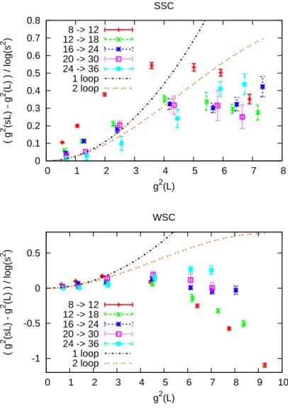
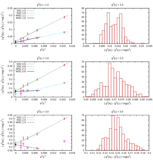
In conclusion it looks very plausible that the SF coupling turns out to be a good probe for IR conformality, however more theoretical work is needed in order to un- derstand its low-energy limit. The SF coupling has been widely used to investigate IR conformality in various theories mostly until 2013, and then it has been almost completely replaced by the much more precise gradient-flow coupling. All SF-coupling studies [141–144] agree on the existence of an IR fixed point inSU(2) with 2 adjoint fermions. Concerning SU(2) with Nf fundamental fermions, the SF-coupling runs away for Nf = 4 [145], and an IR-fixed point is found for Nf = 10 [145]. The case Nf = 6 collects evidence in favour of slow running of the SF-coupling [145, 146] and against it [147]. TheSU(3) gauge theory with 8 fundamental fermions collected evi- dence for strong running of the SF-coupling [64,148]. The same studies report evidence for an IR-fixed point in theSU(3) gauge theory with 12 fundamental fermions. Slow running of the SF-coupling has been reported also in theSU(3) theory with 2 sextet fermions [149–151], in the SU(3) theory with 2 adjoint fermions and in the SU(4) theory with 6 antisymmetric two-index fermions [152] and in theSU(4) theory with 2 symmetric two-index fermions [153].
2.5.4 Gradient flow (GF) coupling
The gauge field Bt at positive flowtimet is defined as a function of the fundamental gauge fieldAthrough the differential equation
∂tBt,µ =Dt,µGt,µν , B0,µ=Aµ , (2.27)
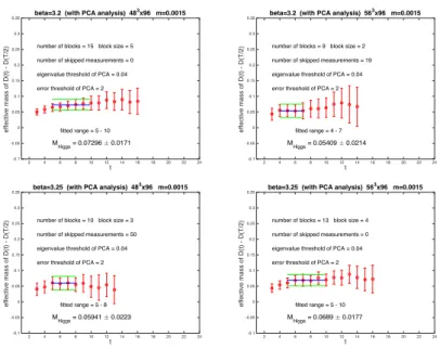
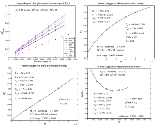
![Figure 4.1: To illustrate cutoff dependent taste breaking effects, spectra of mass- mass-deformed non-Goldstone pion states are shown from our newest data with the definition of the relevant correlators and quantum numbers given in [15,66]](https://thumb-eu.123doks.com/thumbv2/9dokorg/1254140.98013/40.892.198.676.301.650/illustrate-dependent-breaking-deformed-goldstone-definition-relevant-correlators.webp)
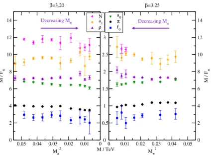
![Figure 8: Schematic view of the emerging resonance spectrum. The parameters and r t are defined in [40].](https://thumb-eu.123doks.com/thumbv2/9dokorg/1254140.98013/43.892.224.647.203.562/figure-schematic-view-emerging-resonance-spectrum-parameters-defined.webp)