S Vesztergom,Eötvös Loránd University, Budapest, Hungary
© 2018 Elsevier Inc. All rights reserved.
Introduction 421
RDEs and RRDEsdPractical Aspects 422
Design 422
Measurements With RDEs 423
Measurements With RRDEs 427
Theory 429
Fluid Flow Under a Rotating Disk 431
Stationary Concentration Profiles and Currents at RDEs 433
Digital Simulation of the RRDE System 436
Charge transfer effects 437
Mass transfer effects 439
IR-drop-related effects 439
Concluding Remarks 443
References 443
Introduction
Electrochemical techniques involving the use of electrodes that move with respect to the solution are commonly termed hydrody- namic techniques. These include configurations where the electrolyte solution is in motion while the electrode itself is stagnant (such as in channelflow systems) or ones where the electrode itself is moved in an otherwise quiescent liquid phase. The most common example of hydrodynamic systems of the latter type is the rotating disk electrode (RDE) or its several variations such as the rotating ring–disk electrode (RRDE).
The advantage of all hydrodynamic methods, irrespective of the actual configuration, is that in such systems steady state can be attained rather quickly and stationary current/potential characteristics can be measured. Also, the rate of mass transfer in a hydro- dynamic configuration is typically higher than that of diffusion alone in nonhydrodynamic systems and this makes the application of hydrodynamic methods extremely expedient, for example, in electrocatalysis research.
Although many hydrodynamic techniques were described in the literaturedthefirst notion about that“movement”has a strong effect on currents measurable during electrolysis was made by Helmholtz1as early as 1880dthe most convenient and widely used system is still the RDE,first described by Levich in 1944.2(Publication in English followed in 1947.3) This electrode is amenable to rigorous theoretical treatment and is easy to construct with a variety of electrode materials.
In what follows I give a brief overview of the most often used hydrodynamic systems: rotating disk and ring–disk electrodes.
As I intended this article to serve as a survey of rotating electrode methods, I did not extend its focus to every detail; however I did wish to highlight some practical aspects that remain unmentioned in other sources. Thefirst part of this article (section“Design”) is thus dedicated to the design of RDEs and RRDEs, as well as to experimental know-how. The basic principles of measurements as well as data analysis strategies are discussed first for RDEs (section “Measurements With RDEs”), then for RRDEs (section
“Measurements With RRDEs”).
Theory underlying the use of rotating electrodes is described in the section“Theory.”Section“Fluid Flow Under a Rotating Disk”contains a description of the hydrodynamics of rotating disk systems, and goes more into details compared to most electro- chemistry textbooks. In section“Stationary Concentration Profiles and Currents at RDEs,”basic analytical expressions (such as the Levich and Koutecký–Levich equations) are derived for RDEs, and I intended this section to be a theoretical supplement to what was said in the section“RDEs and RRDEsdPractical Aspects.”
Finally, section“Digital Simulation of the RRDE System”is dedicated to the theory of the RRDE systems. As from a mathemat- ical point of view RRDEs are generally more complicated than RDEs, my intention in this section was not to derive analytical formulae but rather to demonstrate the use of numerical simulation techniques that can be used for the accurate modeling of RRDE experiments.
For a more detailed introduction to rotating electrode systems, I refer the reader to the electrochemistry textbook of Bard and Faulkner.4For readers who wish for an in-depth understanding, I recommend the famous textbook of Levich5or the excellent review of Gregory and Riddiford6on RDEs, as well as the handbook of Albery and Hitchman7on RRDEs. With respect to the topic of RRDEs, also the papers authored by Albery and his coworkers, which appeared over the 24 years between 1966 and 1989 on the columns of the Transactions of the Faraday Society, are recommended sources.8–31
421
RDEs and RRDEsdPractical Aspects Design
RDEs and RRDEs owe their popularity to their very simple design. RDEs and RRDEs are commercially available, and are both rela- tively simple to construct.
In an RDE, the electrode material (usually some metal or glassy carbon, etc.) is embedded in a rod of insulating material such as Teflon or polyether ether ketone, as shown inFig. 1. The construction of RRDEs, as also shown inFig. 1, is slightly more complicated since in this case a second (ring) electrode material is also applied. The material of the ring can differ from that of the disk: it is however important that the ring should surround the disk electrode concentrically. The gap between the ring and disk materials should befilled by an insulator: usually but not necessarily, the gap isfilled with the same material as that of the outer isolating mantle.
Measurements using conventional RDE or RRDE systems are usually carried out in an electrochemical cell similar to that shown inFig. 2. For accurate measurements it is required that the plane of rotation is aligned horizontally and a large enough cell space is provided so that the natural convection profile remains undisturbed and no turbulence or vortices occur. It is also important to avoid leakage of the solution between the isolating mantle and the electrode material(s).6This necessitates careful construction, especially in the case of RRDEs.
As cells used for RDE or RRDE studies can usually not be made air-tight, measures must be taken to deaerate the solution thor- oughly and to maintain an inert gas blanket over the solution for the time of the experiment, whenever oxygen-free conditions are required. Bubbling gas through the solution during the time of measurement is to be avoided, as this can disturb the convection profile of the rotating electrode.
RDEs and RRDEs are usually rotated at a given rate by a motor that is equipped with a tachometer and a precise control unit.
Rotation rate is often denoted byfand is usually expressed in a unit of revolution per minute (min1or rpm). In practice, rotation rates used in RDE and RRDE studies vary between 100 and 3000 min1. In the mathematical description of RDE systems the angular frequencyuis more often used to express the speed of rotation. The two quantities are related byu¼2pfand the angular frequencyuis usually given in units of hertz (Hz) or s1.
Most rotators available on the market can be used both with RDEs and with RRDEs: in the latter case, the rotator provides two separated electrical contacts, one for the disk and another for the ring electrode. Between thefixed and moving parts of the rotator units, electrical contact is usually provided either by carbon brushes or by mercury slip rings. Mercury contacts exhibit lower resis- tance and are less prone to noise than carbon brushes; however environmental and health hazards must be considered when using mercury-containing rotators. Such rotators are, for obvious reasons, not user-serviceable (and generally do not even require regular maintenance). On the other hand, carbon brush rotators do require maintenance, which involves the regular cleaning of the metallic commutators of the rotating shaft (parts which are contacted by the carbon brushes) by a cloth wetted with isopropanol, and the scheduled replacement of worn-out carbon brushes. Note that new carbon brushes need to be broken in (by rotation lasting
Fig. 1 Sketch of a rotating disk (RDE) and a rotating ring–disk electrode (RRDE) tip. Parts of the electrode tipsd1: disk electrode material;2: ring electrode material;3: insulator;4: metal support. Dimensionsdr1: disk radius;r2: inner ring radius;r3: outer ring radius;r0: overall radius of the tip.
a few hours) to assure good contact to the shaft. In case an RDE or RRDE measurement seems noisy, checking the carbon brushes should always be thefirst step of trouble-shooting.
Measurements With RDEs
RDE experiments do not substantially differ from any other electrochemical studies that involve a standard three-electrode cell (Fig. 2), except that with RDEs, different rotation rates can be set and the dependence of current on rotation rate can be analyzed.
As opposed to quiescent systems, RDEs facilitate the measurement of truly stationary polarization curves; however they can also be used for the application of transient techniques such as linear sweep voltammetry.
For electrochemical systems where mass transfer (the diffusion of dissolved species) does not play any prominent role in deter- mining the measurable current/voltage characteristics, the response measurable on an RDE should be very similar to that detected on stagnant electrodes. An example is shown inFig. 3, exhibiting only slight differences between the cyclic voltammograms of the Au(poly)|H2SO4(aq) system, measured when the electrode is stagnant (curve1) and when it is rotated (curve2).
Fig. 2 Scheme of an electrochemical cell with a rotating disk electrode controlled by a simplified potentiostat circuit. Parts of the celldWE, working electrode (RDE);CE, counter electrode;RE, reference electrode;L, Luggin capillary;GF, glass frit separating the counter and working electrode compartments;G, gas inlet. Parts of the potentiostatdOA, operational amplifier that keeps the potential of REvs.WE (that is,E) at a constant set-point levelEPRby passing a currentIthrough the WE–CE loop.A and V, current and voltage meters.
Fig. 3 Cyclic voltammograms (already attained theirfinal shapes) of a polycrystalline gold disk immersed into a 0.5 mol dm3solution of sulfuric acid, recorded at a sweep rate of 50 mV s1. Curve1was measured on a nonrotating electrode; curve2was measured when the electrode was rotated at 500 min1. Curve3, which is almost fully overlapping with curve1at the present scale, was measured again on a nonrotating electrode, however following the addition of trace amounts of a chloride-containing contaminant. Curve4was recorded in the contaminated cell at 500 min1.
That rotation has practically no effect on this system is in fact not surprising, since the oxidation and the corresponding reduction of a gold surface should not be limited by the mass transfer of any species dissolved in the solution. Nevertheless, introducing rota- tion can still be expedient in order to check the purity of the system: this is because when differences between the response of stag- nant and rotating electrodes do emerge, these often originate from an impurity of the solution.
As also shown inFig. 3, by adding a very small amount of a chloride-containing contaminant to the solution, differences between the voltammetric response of rotating and stagnant electrodes become pronounced. In case of the Au(poly) | H2SO4(aq) system, the cause of this effect is the adsorption of chloride at the electrode surface which hinders its oxidation. As the surface coverage of Clions does depend on the concentration of chloride in the near-electrode solution layer, whether convec- tion can resupply chloride has a deep impact on the measured cyclic voltammograms (CVs). This carries an important practical message for experimenters using hydrodynamic techniques: which is that the utilization of convection always makes sure that impu- rities,whenever present in the system, always end up at the electrode surface, and thus hydrodynamic measurements are often more sensitive to contaminations compared to other electrochemical techniques.
To this statement I add that in convective systems it is also more likely that products of the counter electrode reaction can reach the working electrode surface: therefore, separation of the counter and working electrode compartments (as was shown inFig. 2) is essential.
Most RDE studies focus however not on surface-confined reactions but instead on electrode processes that involve dissolved reactants. In this casefluidflow is rather beneficial as it can provide a continuous supply of the reactants and as a result, on an RDE much larger faradaic currents can be upheld than on stagnant electrodes. In an RDE system, convection also makes sure that the products of the electrode reaction are swept away from the disk surface rather quickly. Consequently, reversal techniques common for quiescent systemsdsuch as CVdare rarely applied to RDEs, although they can very well be used to demonstrate the effect of convection. This is shown by the CVs ofFig. 4, taken at different sweep and rotation rates in a system that contains an oxidized species which can undergo a reversible one-electron reduction.
Fig. 4 Cyclic voltammograms (already attained theirfinal shapes) of a disk electrode that is immersed into a solution containing an oxidized species that can undergo a fully reversible 1-electron reduction in which a reduced species is formed. CVs are recorded at different sweep and rotation rates.
Initially, only the oxidized species are present in the cell.
InFig. 4it is apparent that in a quiescent system (i.e., at 0 min1) a reduction wave and a (reversal) oxidation wave are both present in the CVs and that the peak heights scale linearly with the square root of the sweep rate. On rotated electrodes, however (particularly if the rotation rate is high and the sweep rate is low), the reversal peak vanishes.
Also the cathodic scans of the CVs differ for rotated and quiescent systems inFig. 4. At high rotation and relatively low sweep rates, the peak-like feature of the cathodic scans gets suppressed, as the cathodic currentdinstead of following a slow decaydattains afinite limit. As can be observed inFig. 4, this“limiting current”is proportional to the square root of the rotation rate, and is described as
I‘¼0:620nFAD2=3n1=6cNu1=2: (1)
In Eq.(1),nis the number of electrons transferred in the reaction,F¼96485.3 C mol1is Faraday’s constant,Ais the surface area of the electrode,nis the kinematic viscosity of the solution,cNis the bulk concentration of the reacting species, anduis the angular frequency of rotation. Eq.(1), the famous Levich-equation, is central to rotating disk systems. (Insight to the theoretical background of the important equations used for the analysis of RDE measurementsdsuch as the Levich equation, Eq.(1)and the Koutecký–Levich equation, Eq.(4)dis given in the section“Theory.”)
Although the Levich equation contains only two parameters directly related to the interfacedthe area of the electrodeAand the number of electrons transferred in the electrode reactionnd, and thus it has little to say about the kinetics of the electrode reaction, it still offers a straightforward way for determining bulk parameters of the system. For example, if bothAandn, as well as the bulk concentration of the reacting speciescNand the kinematic viscositynof the electrolyte solution are known, the measurement of limiting currents and their analysis based on the Levich equation can be used for determining the diffusion coefficientDof the react- ing species.
In order to use the Levich equation for the determination of diffusion coefficients, the dependence of the limiting current versus the square root of the rotation rate is to be analyzed. An example is given in Fig. 5A, showing stationary polarization curves measured at different rotation rates in a system that contains an oxidized species undergoing reduction at certain (cathodic) potentials.
For valid analysis, care must be taken during such measurements as to that the polarization curves are trulystationary. This can be achieved either by setting the potential point-by-point, and then determining a constant current corresponding to each potential value or by recording linear sweep voltammograms at different (preferably low) sweep rates and ruling out any sweep rate dependence.
It is apparent inFig. 5A that at not very cathodic potentials (i.e., within the regime of“kinetic control”) the measured current strongly increases with the applied cathodic potential. As the potential is set to more cathodic values, the current increase breaks down and after passing a regime of“mixed control,”current attains a limiting value that is already“transport controlled”dsee the approximate control regime boundaries marked on the colored stripe inFig. 5A.
The underlying physical picture is that at not very negative potentials, the rate of the reaction (i.e., the probability of that an oxidized species near the electrode surface can undergo a reduction event) is relatively small; however it increases with the applied potential. The current versus potential dependence within this“kinetic control”regime is essentially determined by the mechanism
Fig. 5 (A) Stationary polarization curves measured at different rotation rates for a system where an oxidized species (offinite bulk concentration) undergoes reduction at a rotating disk electrode. Selected current values (marked byred dotsandgreen crosses) are plotted on a Levich (B) and on a Koutecký–Levich (C) plot.
of the electrode reaction. In the simplest case one can assume that current depends exponentially on the applied potential, as is described by the Erdey-Grúz–Volmer–Butler equation:
I¼nFAkc0exp anF
RT EEeq
; (2)
where (EEeq) is the overpotential (the difference of the electrode potentialEand its equilibrium valueEeq, often denoted ash), ais the charge transfer coefficient,kis the rate coefficient, andc0is the concentration of the reactantat the electrode surface.
In a system where thebulkconcentration of the reactant (cN) is large enough so that the electrode reaction cannot cause any significant near-surface concentration decrease (that is, c0zcN), the measured current practically coincides with a so-called catalytic current that can be obtained by assuming thatc0¼cNin Eq.(2), and thus
Icat¼nFAkcNexp anFh RT
: (3)
The situation is however different for systems where the bulk concentrationcNof the reacting species is not infinitely high. In such systems, as shown inFig. 5A, the measured polarization curves follow the catalytic current only at low overpotentials. As the overpotential is set to higher values, the driving force of the electrode reaction becomes so large that practically every oxidized mole- cule reaching the electrode surface immediately undergoes reduction. In this case increasing further the overpotential has already no effect on the measured current, as the rate of the reaction is already“transport controlled”dthat is, the reaction rate is limited by the speed at which new reactant species are transported from inside the bulk to the electrode surface, and not by the (practically infinite) rate of the electrode reaction. Naturally, at certain overpotentials both kinetic and transport control have a role in determining current; thus there exists also a“mixed control”regime between the regimes of kinetic and transport control (seeFig. 5A).
In order to use the Levich equation (Eq.1) for the determination of bulk transport parameters, limiting current sections must be attained at all rotation rates. In a practical system, these can be recognized asflat plateaus of the polarization curves; that is, sections where dI=dEz0. By reading the currents at the plateau sections (see the red dots inFig. 5A) and plotting them as a function of the square root of the angular frequency of rotation ffiffiffiffi
pu
ð Þ, one should obtain a straight line with an intercept of zero, as inFig. 5B (red dots and line). The slope of this line (commonly called the“Levich slope”) can then be estimated and used, for example, for calcu- lating the diffusion coefficient of the reacting species from Eq.(1).
In some practical systems, however, the measurement of true limiting currents is not feasible, either due to instrumental limi- tations, due to gas evolution (resulting in noisy curves), or due to the fact that the electrochemical stability window of the system is not broad enough. In the latter case, the onset of additional currents makes the limiting current plateaus ill-defined.
Assume, for example, that the polarization curves ofFig. 5A can only be experimentally determined up to the potentials marked by the green crosses, and that the limiting current sections (for whatever reason) cannot be reached. If we wrongly identify the currents marked by the green crosses as limiting currents, and plot these as a function of ffiffiffiffi
pu
ð Þ, the obtained graph (see the green curve inFig. 5B) will not be linear and any attempt at calculating transport parameters based on a linearfit will ultimately be erro- neous. For valid analysis, we thus need to make use of an alternative method that is based on the Koutecký–Levich equation.
The Koutecký–Levich equation basically states that the current measurable under“mixed control”conditions on an RDE is the harmonic sum of the transport controlled (limiting) and the catalytic (kinetic) currents. That is,
I1¼I1‘ þI1cat: (4)
A rigorous mathematical derivation of the Koutecký–Levich equation will be given in the section“Theory”; for a mere qualitative understanding it is enough to makeFig. 5A subject to closer inspection. It is apparent here that the higher rotation rates we apply, the closer the obtained polarization curves will lie to the (theoretical)“catalytic current.”In fact, we can reason that by applying an infinitely large rotation rate, in lieu of any transport limitation, the measured current should coincide completely with the catalytic current given in Eq.(3).
Naturally, infinite rotation rates are not practically applicable; nonetheless we can use extrapolation. To do so, in accordance with the Koutecký–Levich equation, we plot the reciprocals of currents measured at the same potential but at different rotation rates (green crosses inFig. 5A) as a function ofu1/2. As a result we obtain the straight green line shown inFig. 5C. The intercept of this straight line (i.e., the inverse current corresponding to infinite rotation rates) gives the reciprocal catalytic currentIcat1, analyzing the potential dependence of which may shed light on the mechanism of the electrode reaction. The slope of the straight line, on the other hand, equals the“inverse Levich slope”(0.620nFAD2/3n1/6cN)1and contains bulk transport properties such as the diffusion coefficient.
As we see, analysis based on the Koutecký–Levich equation tells more about the system under study than the Levich equation alone, since it also enables the determination of kinetic parameters. If we apply the Koutecký–Levich analysis to currents that are fully transport-limited (red dots and line inFig. 5A), we still get a straight line with the same“inverse Levich slope”as before, but with an intercept of zero (Fig. 5C). From our previous reasoning it follows that at these potentialsIcat1z0 and thus, the catalytic current (at least in comparison to the mass transfer limitations present in the system) can be considered practically infinitedyet the slope still allows us to determine parameters related to transport, just as the“simple”Levich equation would do.
I add that linearizing the Koutecký–Levich equation as in Eq.(4)is not absolutely necessary. By utilizing the fact that in case of mixed kinetics (subject to both catalytic and mass transfer limitations) the measured current is the harmonic sum of the catalytic
and transport-related currents, stationary polarization curves measured at different rotation rates can directly be made subject to nonlinear parameter estimation. In order to do so, one has to construct a model based on which an equation for the catalytic current (such as the one in Eq.3) can be derived. For example, for the polarization curves ofFig. 5A one could assume that current (at a given overpotentialh¼EE0and angular frequencyu) is defined as
Iðh;uÞ ¼ nFAcN
1
kexpðan FhRTÞ þ0:620D2=31v1=6u1=2: (5)
While some parameters of Eq.(5)(n,A,cN,T,n) are usually known to the experimenter, other parameters (usuallyk,a, andD) can be varied and optimized tofit the polarization curves. For correct parameter optimization it is not strictly required that the polarization curves attain well-defined limiting current plateaus; reaching these, however, helps a lot in minimizing the error of optimization and the correlation of parameters.
Note that while the Levich equation (Eq.1) only holds for limiting currents (that have essentially no potential dependence), analyses utilizing the Koutecký–Levich equation always necessitate a well-defined potential scale. That is, for the determination of kinetic parameters one needs to read currents at exactly defined electrode potential values. Consequently,IRdrop effects must either be compensated or corrected for postexperimentally, or measures should be taken that no considerableIRdrop occurs in the system. The latter can be achieved by using well-conducting electrolytes and by minimizing the distance (without disturbing theflow profile!) of the Luggin capillary and the working electrode surface.
As can be seen above, the analysis of RDE measurements can be expedient in determining important parameters both of elec- trode reactions and of transport in the bulk. A few examples to such analyses can be found among the Refs. [32,33].
Measurements With RRDEs
As it was already pointed out before (cf.Fig. 4), reversal techniques are not available with RDEs, since the product of the electrode reaction is continuously swept away from the surface of the disk.4Information equivalent to that available from reversal techniques at a stationary electrode can be obtained by the addition of a second electrode, as was shown inFig. 1. The thus formed RRDE (first described by Frumkin in 195934) has become one of the most convenient and widely used tools of determining electrode reaction pathways.7
As a typical example of so-called generator–collector assemblies, RRDEs are often used for the detection of products and inter- mediates formed in electrode reactions. Products formed at the disk (generator) electrode leave the disk surface and due to forced convection make their way toward the ring electrode (collector). The potential of the ring,Ering, can be regulated independently from the potential of the disk,Edisk; that is, when an appropriate value ofEringis used, the portion of disk reaction products reaching the ring electrode can undergo another electrode reaction and can thus be detected.
In an RRDE, the current–potential characteristics of the disk are unaffected by the presence of the ring and the properties of the disk are as described in the section“Measurements With RDEs.”In fact, if the disk current is found to change upon variation of the ring potential or current, one should suspect either a defective RRDE (direct leakage between the disk and ring electrodes) or an undesirable electrical cross-talk35–37due to the coupling of the ring and disk through the uncompensated solution resistance. Effects related to electrical cross-talk are going to be discussed later in the section“Digital Simulation of the RRDE System”where it will be shown that the appearance and intensity of these effects depend heavily on the placement of the reference electrode (i.e., the tip of the Luggin capillary) within the cell.
Since RRDE experiments involve the examination of two potentials (EdiskandEring) and two currents (IdiskandIring), the repre- sentation of the results involves more dimensions than for experiments involving a single working electrode.4RRDE experiments thus rely on more complex instrumentation than RDE studies and require the use of a bi-potentiostat.
Thefirst bi-potentiostat (actually, for RRDE measurements) was developed by Napp et al. in 1967. In the past few decades, several improvements have been made to these devices, which resulted in a higher bandwidth, stability of response, and conve- nience. A simplified circuit of a modern bi-potentiostat (PINE AFRDE538) is shown inFig. 6. The circuitry of the potentiostatic control of the disk electrode consists of the potential follower PF1 and the control amplifier CA1 (the output of which is connected to the counter electrode), and the current-to-voltage converter CTV. Serving as a current sink, CTV keeps the disk electrode at virtual ground by means of its current feedback loop; meanwhile, the amplifier CA1 maintains the difference between the disk and the reference electrode at the desired value. The circuitry required for the potentiostatic control of the second electrode (the ring) consists of the potential follower PF1, the inverter I, the control amplifier CA2, and the potential follower PF2. The role of CA2 is to make the potential difference between the ring electrode and the reference electrode equal to the voltage of the excitation signal.
As it can be seen inFig. 6, the counter electrode is included in the control loops of both working electrodes; the current thatflows through it is thus the algebraic sum of the disk and ring currents. By the application of a circuit like this, simultaneous potential control of the two working electrodes can be achieved. In many cases, however, an equally efficient bi-potentiostatic control can also be achieved by using two“single”potentiostats instead of a bi-potentiostat. The technical feasibility of this approach depends on the grounding concepts of the devices; that is, two or more potentiostats can be used in a multipontetiostat assembly provided that their circuits ground the counter (or, alternatively, the reference) and not the working electrode. For example, the XPot poten- tiostats manufactured by Zahner Messsysteme, Kronach, Germany39can be operated by placing the counter electrode to ground;
thus these devices can be used to create a bi-potentiostatic setup.
The ability of controlling two electrode potentials independently creates a myriad of possibilities for using RRDEs; the usual approach is however to keep either one (or both) of the electrodes at constant potential or current.
For example, when using an RRDE one can record a current–potential curve (e.g., a CV) on the disk electrode, while keeping the ring at a constant potential and observing changes of the ring current. This can lead to the detection of disk-originated products, such as in case of the surface oxidation/reduction of gold electrodes,40–42where by keeping the ring electrode at suitably low potentials, the formation of a reducible intermediate (an oxidized gold species) can be detected (seeFig. 7).
Fig. 6 Circuit schematics of a bi-potentiostat coupled to an electrochemical cell holding an RRDE, a counter, and a reference electrode.
Fig. 7 (A) Cyclic voltammograms measured on the disk electrode of a gold disk–gold ring RRDE, immersed into a 0.5 mol dm3H2SO4solution.
CV vertices: 1400 and500 mV versus SCE, sweep rate: 50 mV s1. (B) The ring current recorded in parallel with measuring the CVs of the disk, plotted as a function of the disk potential, reveals the formation of reducible intermediates accompanying both the oxidation and the subsequent reduction of the gold surface. Rotation rate: 500 min1, ring potential: 0 V versus SCE.
Alternatively, one may also choose to holdEdisk(orIdisk) at a constant value, and scan the ring potential: this allows the iden- tification (and detection) of multiple products. Such experiments were carried out, for example, by Kamar and Miller43to study the corrosion of La2CuO4in aqueous media.
In the above-mentioned“collection”experiments, the aim is to bring a disk-generated product into reaction at the ring surface. It is important to note, however, that only a certain ratio of disk-generated products can get close to the ring electrode: some amount necessarily diffuses away toward the bulk solution and escapes detection. In order to express this behavior, one can define a“col- lection efficiency”for RRDE systems.
In practice, the collection efficiencyNis measured under well-defined conditions. For example, in a system that contains a reduc- ible species, one can set a disk potential that is negative enough so that at a certain rotation rate a cathodic (limiting) current can be measured. In the meantime, the ring potential can be set to positive values so that any reduced product formed on the disk, when reaching the ring electrode, would immediately be oxidized back. The collection efficiency can then be defined as
N ¼Iringndisk
Idisknring; (6)
wherendiskandnringdenote the number of electrons transferred in the disk and ring electrode reactions. (Note that in most cases, nring¼ ndisk.) By definition,N is a positive number less than unity; usual values range between 25% and 37%.
In measurements we usuallyfind that at high enough rotation rates, the collection efficiencyNdoes not depend on the applied rotation rate and is only a function of the geometric parameters of the RRDE. A theoretical expression forN was derived in 1966 by Albery and Bruckenstein8:
N ¼1Fða=bÞ þb2=3ð1Fð ÞaÞ ð1þaþbÞ2=3 1F aþa2þab b
; (7)
where
a¼ r2 r1
3
1; (8)
b¼r33 r31r23
r13; (9)
and the functionF(q) is defined as Fð Þ ¼q
ffiffiffi3 p
4pln 1þ ffiffiffi
3q
p 3
1þq
! þ 3
2parctan 2 ffiffiffi
3q p 1
ffiffiffi3 p
! þ1
4: (10)
(For the dimensionsr1,r2,andr3, seeFig. 1.)
RRDE experiments are not always conducted in a collection mode: sometimes, RRDEs are also used to study shielding. In shield- ing experiments, the ring is set to a potential value where bulk species react on its surface yielding a currentIring0when the disk is not polarized. Then, by setting the disk electrode also to a potential where the same reaction occurs, this will reduce the current measur- able on the ring electrode (as a portion of the reactants which could otherwise reach the ring would now react on the disk). In this case the measurable ring current is
Iring¼Iring
0 NIdisk: (11)
Although most of the standard RRDE techniques involve static control (at least at one of the electrodes), and thus these tech- niques focus on the study of either collection or of shielding effects, recent advances in the instrumentation of RRDE systems also enable the simultaneous study of both effects.44This necessitates the application of potentiodynamic control of both the disk and the ring electrode at the same time. For example, by a slow scanning of the disk potential and a synchronous high-rate cycling of the ring, shielding and collection effects accompanying oxygen reduction on gold were analyzed45(seeFig. 8).
Theory
As I pointed out before, RDEs (and RRDEs) owe their popularity to the fact that measurements involving them can be modeled relatively simply.
When modeling electrode processes, our aim is usually to derive mathematical expressions that can predict measured results; for example, for RDEs, stationary polarization curves like those shown inFig. 5A. To do so, we have to consider and describe in a math- ematical form the electrode reaction. Then we need to consider the effect of mass transfer in the solution phase that resupplies reac- tants to the electrode reaction and also takes products away. Transport, by nature, is a space-dependent process, while the electrode reaction is confined to a certain plane (the electrode surface). Thus what we usually do when modeling electrode processes is that we aim to solve the equations of transport under certain boundary conditions that are determined by the electrode reaction. This can
result in the determination of (either stationary or time-dependent) concentration profiles for the species involved in the electrode process. Knowing the profiles, determining currents is just one step ahead.
The physical laws describing mass transfer dictate that theJiflux of a speciesi(i.e., the amount of substance dnithat passes a certain, arbitrarily chosen areaAwithin an infinitesimal time-step dt) is determined as
Ji¼1 A
dn
dt¼ DigradciþcivþziFDici
RT gradfþother terms: (12)
That is,flux is determined by the rate of diffusion, convection, and migration, as described by the three terms in Eq.(12); in some cases other terms (e.g., describing homogeneous reactions in the bulk) can also be added. In what follows we will only focus on problems where homogeneous reactions do not occur and the effect of migration (i.e., the movement of a species carryingzicharge in response to an electricalfieldf) is also neglected. Thus, our considerations will only apply to systems that contain a supporting electrolyte in large concentration, shielding the electric potential so that gradf¼0. This leaves us with only two terms present on the right-hand side of Eq.(12). Eq.(12)now tells us that when a certain amount of substance moves through a given surface areaA in the system, then this movement is either due toflow (of velocityv) or due to diffusion. Note that in the absence of convection (v¼0), Eq.(12)reduces to Fick’sfirst law of diffusion.
Let us assume now that the areaAwe choose to write Eq.(12)for (this can be chosen arbitrarily) is that surrounding a closed volumeV.We can now arguedsince chemical reactions are not taking placedthat any change of the amount of substance within this volumeVcan only occur if some amount of substance leaves or enters the bounding areaA. That is, by integrating concentration changes inside the volumeVoverV, we must get the same result as if we would integrate theflux over the areaA, or (by using the Gauss–Ostrogradsky theorem) if we would integrate the divergence of theflux overV.That is,
Z
V
vci
vtdV¼I
A
JidA¼Z
VdivJidV: (13)
From this and from the remaining terms in Eq.(12)it follows that vci
vt ¼divðDigradciÞ divð Þ;civ (14) or, if we assume that the diffusion coefficientDiis a constant independent of space and thefluid is incompressible so that divv¼0,
vci
vt ¼Didiv gradciv$gradci: (15)
When dealing with hydrodynamical techniques, the convective–diffusion equation we usually aim to solve is Eq.(15). The solu- tion then yields concentration profiles based on which theflux of the different species at the electrode surface can be calculated (using Eq.12) andfinally, the current can be determined.
In order tofind a solution for Eq.(15), expressions for the velocity profilevmust be obtained. Generally,v¼v(x,t) is a vector field that depends both on time and spatial coordinates; however in many cases (such as for the majority of rotating electrode tech- niques) we assume that theflow is stationary.
Fig. 8 (A) The shape of the CVs measured on the ring change when oxygen reduction occurs on the disk electrode of an Au–Au RRDE in an air-saturated 0.5 mol dm3sulfuric acid solution. The polarization curve obtained from the disk and a few ring CVs are shown together. (B) Changes of the ring CVs (vs.the“reference CV”shown in (A)), visualized as a function of the disk and ring potentials. The“3D map”of the oxygen reduction process reveals both the shielding of the ring that arises from the reduction of oxygen at the disk, and also an anodic peak that is caused by the oxidation of the hydrogen-peroxide formed at the disk. For details of the experiment, see Ref. [45].
Fluid Flow Under a Rotating Disk
In an incompressiblefluid,flow profiles are described by the Navier–Stokes equation dv
dt¼ gradp
9þvdiv gradvþf
9 (16a)
and the equation of continuity,
divv¼0: (16b)
The simple form of the Navier–Stokes equation given in Eq.(16a)is in fact a formulation of Newton’sfirst law for a given solu- tion volume. It states that any acceleration of the fluid dv=dt
arises from the negative gradient of pressure over density gradp=9
as well as from any outer forcefapplied to thefluid (normalized with the density9). Velocity losses arise as a result of dissipation of the kinetic energy due to internal friction, as represented by the termndiv gradv, wherenis the kinematic viscosity of the liquid.
The theoretical treatment of RDEs requires the solution of the Navier–Stokes equation for a system that consists of an infinitely large disk rotating in a viscous medium. This problem wasfirst studied and solved by the Hungarian scientist Tódor Kármán in 1921,46followed by a more accurate solution of Cochran in 1934.47The results of Kármán and Cochran were used by Levich when formulating the theory of RDEs.5
The symmetry of the rotating disk system suggests that the problem should be treated using cylindrical coordinates, as shown in Fig. 9. In order to describe theflow profile, we place a disk of infinite radius (i.e., a suitably large disk) centered on the origin of the coordinate system, with its axis of rotation aligned to thez-axis. (A practical consequence of the assumptions taken for solving the Navier–Stokes equations is that the rotated mantle should be appropriately thick: usually, the dimensionr0>0.5 cm (seeFig. 1).) If we write out the differential operators in Eqs.(16a) and (16b)using cylindrical coordinates, we obtain the following system of partial differential equations that describe thevr,v4, andvzvelocity components:
vvr z}|{0ðiÞ
vt þvrvvr
vr þv4 r
vvr
v4 zfflffl}|fflffl{0ð Þii
þvzvvr
vzv42 r ¼ v
vr p
|fflfflfflffl{zfflfflfflffl}9
0ð Þiii
þn 1 r
v vr rvvr
vr
þ1 r2
v2vr
v42
|fflfflfflffl{zfflfflfflffl}
0ð Þiii
þv2vr
vz2 vr
r22 r2
vv4
|fflfflffl{zfflfflffl}v4
0ð Þiii
2 66 64
3 77 75þ fr
|{z}
0ð Þiv
(17a)
vv4
z}|{0ð Þi vt þvrvv4
vr þv4 r
vv4
v4 zfflfflffl}|fflfflffl{0ð Þii
þvzvv4
vz vrv4 r ¼ 1
r v v4
p
|fflfflfflfflfflffl{zfflfflfflfflfflffl}9
0ð Þiii
þn 1 r
v vr rvv4
vr
þ1 r2
v2v4 v42
|fflfflfflffl{zfflfflfflffl}
0ð Þiii
þv2v4 vz2 v4
r22 r2
vvr
|fflfflffl{zfflfflffl}v4
0ð Þiii
2 66 64
3 77 75þ f4
|{z}
0ð Þiv
(17b)
vvz
z}|{0ð Þi vt þvrvvz
vr zffl}|ffl{0ð Þv
þv4 r
vvz
v4 zfflffl}|fflffl{0ð Þii
þvzvvz
vz ¼ v vz
p 9 þn 1
r v vr rvvz
vr
|fflfflfflfflfflfflfflfflffl{zfflfflfflfflfflfflfflfflffl}
0ð Þv
þ1 r2
v2vz
v42
|fflfflfflffl{zfflfflfflffl}
0ð Þiii
þv2vz
vz2 2
66 64
3 77 75þ fz
|{z}
0ð Þiv
(17c)
0¼1 r v
vrð Þ þrvr 1 r
vv4
|fflffl{zfflffl}v4
0ð Þiii
þvvz
vz (17d)
Fig. 9 A system of cylindrical coordinates showing a pointPof coordinatesr,4, andz. The disk is placed in thex yplane, rotating around the point atr¼0 with constant angular velocityu.
Inspection of Eqs.(17a)–(17d)reveals that several terms cancel out because of either one of the following reasons:
(i) All temporal derivatives are considered zero: this will lead to a solution for the stationaryflow profile.
(ii) All derivatives with respect to the angular coordinate4vanish due to the axial symmetry of the system.
(iii) Due to the horizontal alignment of the disk, the derivative of pressurepwith respect to the radial coordinatervanishes.
(iv) External forces (such as due to gravity) are considered negligible so that all entries of the vectorfare treated as zero.
(v) Since the disk is considered infinitely large, the axial velocity component is independent of the radial coordinate and thus vvz=vr¼0.
The above considerations, when used to simplify Eqs.(17a)–(17d), result in the following system of partial differential equations describing stationaryflow:
vrvvr
vr þvzvvr
vz v24 r ¼n 1
r v vr rvvr
vr
þv2vr
vz2 vr
r2
(18a)
vrvv4 vr þvzvv4
vz vrv4 r ¼n 1
r v vr rvv4
vr
þv2v4 vz2 v4
r2
(18b)
vzvvz vz ¼ v
vz p
9 þnv2vz
vz2 (18c)
0¼1 r
v
vrð Þ þrvr vvz
vz (18d)
To solve Eqs.(18a)–(18d), we formulate two boundary conditions. One of these is a so-called no-slip condition at the surface of the disk; that is, thefluid layer adjacent to the rotating disk surface moves together with it, and thus
vr¼0; v4¼ur and vz¼0 at z¼0: (19)
That the rotating disk drags the nearbyfluid layer (which then moves together with the disk) implies that there is a significant radial velocity at not very high distances below the rotating surface, in the direction outward from the axis of rotation. Due to the requirement of continuity, this radial outflow must be compensated by an axial inflow that shoulddsince the disk is infinitely or, at least in practice, very largednot depend on the radial coordinate. This results in the following boundary condition:
vr¼0; v4¼0 and vz¼ vN at z¼N: (20)
By introducing at this point the dimensionless variable z¼z
ffiffiffiffiu v r
(21) and the scaling functionsF(z),G(z),H(z), andP(z) so that
vr¼ruFð Þ;z (22a)
v4¼ruGð Þ;z (22b)
vz¼ ffiffiffiffiffiffi pvu
Hð Þ;z (22c)
p¼ 9vuPð Þ;z (22d)
the system of partial differential Eqs.(18a)–(18d)can be cast into the following system of ordinary differential equations:
F2þF0H¼F00þG2 (23a)
2FGþG0H¼G00 (23b)
2FþH0¼0 (23c)
HH0¼P0þH00: (23d)
Note that the scaling function for pressure,P(z), appears only in Eq.(23d)and thus this equation can be decoupled from the system of ordinary differential equations(23a)–(23c)describing theflow velocity components. Unfortunately, no exact solution was found so far for this system of equations. In 1934, Cochran provided an approximate solution in the form offinite-term series and by optimizing the coefficients.47More than 80 years later it seems simpler (and more accurate) to look for a numerical solution.
A numerical solution to Eqs.(23a)–(23c)can be found by assuming we know what initial values (atz¼0) the functionsF,G, andHas well as the derivativesF0andG0take. ThenH0(0) can already be found from Eq.(23c)and values of the second derivatives
F00(0) andG00(0) can also be expressed from Eqs.(23a) and (23b), respectively. Knowing these initial values we could then start an iteration, increasing in each step the independent variablezby small steps of
O
zand determining in eachkth step new function and derivative values, based on values defined in the previous step (k1). That is,Fk¼Fk1þDzFk10 (24a)
Gk¼Gk1þDzG0k1 (24b)
Hk¼Hk1þDzH0k1 (24c)
F0k¼Fk10 þDzFk100 (24d)
G0k¼G0k1þDzG00k1 (24e)
and then,
H0k¼ 2Fk (24f)
F00k ¼F2kþFk0HkG2k (24g)
G00k¼2FkGkG0kHk: (24h)
This iteration, started fromz¼0, can be used to generate numerical values atfineDzsteps for the functionsF,G, andH. All it requires is the knowledge of theF(0),G(0),H(0),F0(0), andG0(0) initial values.
The only problem of the above method is that some of the initial values are not known. The boundary conditions given by Eqs.
(19) and (20), when written for the dimensionless scaling functions, translate to Fð Þ ¼0 0; Gð Þ ¼0 1; Hð Þ ¼0 0; lim
z/NFð Þ ¼z 0 and lim
z/NFð Þ ¼z 0: (25) That is, instead of having initial values for the derivativesF0andG0, we havefinal values (asz/N) for the functionsFandG. In order to stillfind a numerical solution for Eqs.(23a)–(23c), we thus utilize the so-called shooting method. This requires that we make an initial guess for the values ofF0(0) andG0(0) and then do an iterative solution which goes to large values ofz. The obtained FandGfunctions will probably not reach 0 (as they should) whenztends to infinity; however in subsequent iterations we can modify the initial guess and improve the asymptotic behavior.
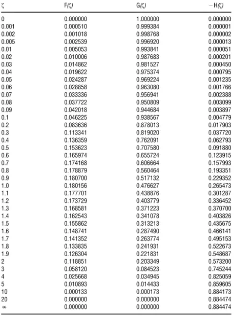
The shooting method results in reliable solutions for the functionsF,G, andHthat are tabulated as a function ofzinTable 1.
Based on Eqs.(22a)–(22c), the velocity profile componentsvr,v4, andvzcan be calculated using the function values listed inTable 1 for given values ofnandu.
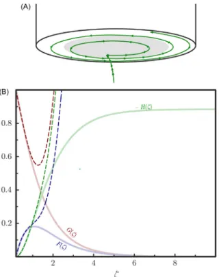
Fluid motion due to convectiveflow is illustrated byFig. 10A: here a chosenfluid volumefirst approaches (mostly by movement in thezdirection), then leaves (by radial out-drift) a disk electrode rotated as part of a larger plane.
The functionsF(z),G(z), andH(z) are plotted versuszinFig. 10B. Here the series approximations of Cochran,47valid forz1, are also shown (see the dashed lines inFig. 10B):
Fð Þ ¼z azz2 2 bz3
3 þ/ (26a)
Gð Þ ¼z 1þbzþaz3
3 þ/ (26b)
Hð Þ ¼ z az2þz3 3þbz4
6 þ/ (26c)
The coefficients in Eqs.(26a)–(26c)were determined by Cochran47asa¼0.51023 andb¼ 0.6159.
Stationary Concentration Profiles and Currents at RDEs
Once the velocity profile has been determined, the convective–diffusion equation, Eq.(15), can be solved for the RDE. First we point out that RDEs (provided that not only the rotating shaft but also the electrode has a large enough radius) can in almost all cases be safely treated as one-dimensional systems. That is, the current of a large enough RDE will not be affected by radial trans- port, and thus Eq.(15)dassuming only one transferred speciesdsimplifies to
vc vt¼Dd2c
dz2vzdc
dz; (27)
which is a differential equation for one dimension (containing only thezspatial coordinate). Let us now focus on the determination of the stationary profile (for whichvc/vt¼0) and expressvzusing Eq.(22c)and thefirst-term approximation of Eq.(26c). By this we arrive to the following ordinary differential equation determining the stationary concentration profile:
0¼Dd2c dz2þaz2
ffiffiffiffiffiffiffi u3
v
r dc
dz: (28)
The general solution of this differential equation is a function of the form c zð Þ ¼c21
3zc1E2=3 az3 3Di
ffiffiffiffiffiffi u3 v
r !
: (29)
The functionEp(x), appearing in Eq.(29), is called the generalized exponential integral function and it is defined by the integral Ep(x)¼!1Nupexp (xu)du. The generalized exponential integral function is related by the formulaEp(x)¼x(p1)G(1p,x) to the (upper) incomplete gamma functionG(s, x), defined asG(s,x)¼!Nxus1exp (u)du. In Eq.(29),c1andc2are integration constants defined as
c2¼ lim
z/Nc zð Þ ¼cN (30)
Table 1 The scaling functionsF(z), G(z),and–H(z) evaluated at different values of the dimensionless variablez
z F(z) G(z) H(z)
0 0.000000 1.000000 0.000000
0.001 0.000510 0.999384 0.000001
0.002 0.001018 0.998768 0.000002
0.005 0.002539 0.996920 0.000013
0.01 0.005053 0.993841 0.000051
0.02 0.010006 0.987683 0.000201
0.03 0.014862 0.981527 0.000450
0.04 0.019622 0.975374 0.000795
0.05 0.024287 0.969224 0.001235
0.06 0.028858 0.963080 0.001766
0.07 0.033336 0.956941 0.002388
0.08 0.037722 0.950809 0.003099
0.09 0.042018 0.944684 0.003897
0.1 0.046225 0.938567 0.004779
0.2 0.083636 0.878013 0.017903
0.3 0.113341 0.819020 0.037720
0.4 0.136359 0.762091 0.062793
0.5 0.153623 0.707580 0.091880
0.6 0.165974 0.655724 0.123915
0.7 0.174168 0.606664 0.157993
0.8 0.178879 0.560464 0.193351
0.9 0.180700 0.517132 0.229352
1.0 0.180156 0.476627 0.265473
1.1 0.177701 0.438876 0.301287
1.2 0.173729 0.403779 0.336452
1.3 0.168581 0.371223 0.370700
1.4 0.162543 0.341078 0.403826
1.5 0.155862 0.313213 0.435675
1.6 0.148741 0.287490 0.466141
1.7 0.141352 0.263774 0.495153
1.8 0.133835 0.241931 0.522673
1.9 0.126304 0.221831 0.548687
2 0.118851 0.203349 0.573200
3 0.058120 0.084523 0.745244
4 0.025668 0.034945 0.825059
5 0.010893 0.014433 0.859605
10 0.000133 0.000173 0.884173
20 0.000000 0.000000 0.884474
N 0.000000 0.000000 0.884474
and
c1¼ lim
z/0þ
dc zð Þ
dz ¼c0ð Þ:0 (31)
That is, the integration constantc2is in fact the bulk concentration of the reacting speciescNandc1is the gradient of the concen- tration profile at the position of the electrode plane,c0(0). It is also expedient to express the near-surface concentration valuec0as
c0¼ lim
z/0þc zð Þ ¼cND1=3v1=6c0ð Þ0G13;0
32=3a1=3u1=2 : (32)
From Eq.(32), the integration constantc0(0) can be expressed in terms ofc0and can directly be plugged into Eq.(29)to yield a concentration profile parametrized by the near-surface concentrationc0and the bulk concentrationcN:
c zð Þ ¼cNðcNc0ÞG 13; az3D3up3=2ffiffiv
G13;0 : (33)
Concentration profiles for two different near-surface and bulk concentration ratios (c0/cN¼0 and 0.5) are plotted inFig. 11.
Note that inFig. 11 the dimensionless concentrationc/c0is plotted against the distance measured from the electrode surface, expressed here in multiples of the so-called diffusion layer thicknessd.
As shown by the dashed lines inFig. 11,dis the distance where thefirst-order approximations of the concentration profiles inter- sect with the value ofcN. The diffusion layer thickness, as can be seen in thefigure, is independent from the actual value ofc0and of cN.
Mathematically, the diffusion layer thicknessdcan be expressed by expanding Eq.(33)aroundz¼0 to thefirst order, equating the thus-obtained expression tocNand then solving forz. This gives
d¼v1=6G13;0 D1=3 32=3a1=3 ffiffiffiffi
pu z1:6117v1=6D1=3u1=2: (34)
Having determined the concentration profiles, expressing the stationary current measurable on RDEs is just a single step forward.
At this point I refer back to Eq.(12), which states that theflux of a species (through a given surfaceA) is determined as a sum of diffusive and convective (sometimes also migration-related and other) terms. Since the current of the RDE is in fact theflux of the reacting species scaled bynF(wherenis the number of electrons transferred in the electrode reaction andFis Faraday’s constant), the current of the RDE is
Fig. 10 (A) The trajectory of a chosenfluid volume thatfirst approaches (mostly by movement in thezdirection), then leaves (by radial out-drift) a disk electrode rotated as part of a larger plane. (B) The scaling functionsF(z), G(z),andH(z),evaluated at different values of the dimensionless variablez. Approximative solutions given by Eqs.(26a)–(26c)are shown by the dashed curves.
I¼nFADc0ð Þ0 (35) where, for the sake of simplicity, we now assumed that there is only one electrode reaction taking place. By expressingc0(0) from Eq.
(32)and substituting to Eq.(35)we arrive to
I¼nFA cðNc0Þ32=3a1=3D2=3u1=2
v1=6G13;0 ¼nFADcNc0
d : (36)
When limiting currents are measured (i.e., when the reaction is so fast thatc0¼0), Eq.(36)reduces to the Levich equation (Eq.
1) and gives
I‘¼nFAcN32=3a1=3D2=3u1=2
v1=6G13;0 z0:620nFAD2=3v1=6cNu1=2: (37) It follows from Eq.(36)and from the definition of the limiting current, Eq.(37), that for non-limiting stationary currents the equation
I
I‘¼cNc0
cN (38)
holds. Provided that the current of the charge-transfer reaction is scaled linearly with the near-surface concentration (as it is true for Eq.2), we are always able to define a catalytic current (such as we did in Eq.3) that scales linearly withcN. The measurable currentI is then always smaller than the catalytic currentIcat, and
I Icat¼c0
cN: (39)
Uniting Eqs.(38) and (39)then yields the Koutecký–Levich equation, Eq.(4).
Digital Simulation of the RRDE System
As it was shown earlier, deriving closed-form expressions (like the Levich and Koutecký–Levich equations) useful for the analysis of RDE measurements was relatively simple. This is due to the fact that in most cases, RDE systems can be treated as one-dimensional problems. The same cannot be said for RRDEs; in order to describe RRDEs, it is essential to take mass transfer fully into consider- ation (also in the radial, not only in the axial direction).
As a result, deriving closed-form expressions for RRDEs may become overly complicated (although not necessarily impossible:
e.g., Eq.(7)defining the collection efficiency of RRDEs was derived analytically8). Digital simulations offer, however, a possible alternative for the description of RRDE systems and nowadays several software packages are available which can make such simu- lations straightforward. Therefore, in what follows I shall attempt to give an introduction to the simulation of the RRDE systems.
Several such simulationsdof varying scope and accuracydwere devised in the past48,49: the approach we follow here was described in detail in Refs. [50,51].
Fig. 11 Dimensionless stationary concentration profiles for an RDE, plotted as a function of dimensionless distance (distance is expressed as multiples of the diffusion layer thickness defined by Eq.(34)). For the profiles plotted by the red and the green curves,c0¼0 andc0¼c2 ,N
respectively. First-order series approximations are shown by the slanted dashed lines: note their intersection with thecNlevel at 1d.