Practical application of spatial ecosystem service models to aid decision support
Grazia Zulian
a,⇑, Erik Stange
f, Helen Woods
c, Laurence Carvalho
c, Jan Dick
c, Christopher Andrews
c, Francesc Baró
d,e, Pilar Vizcaino
a, David N. Barton
g, Megan Nowel
g, Graciela M. Rusch
h, Paula Autunes
i, João Fernandes
i, Diogo Ferraz
i, Rui Ferreira dos Santos
i, Réka Aszalós
j, Ildikó Arany
j, Bálint Czúcz
j,k, Joerg A. Priess
l, Christian Hoyer
l, Gleiciani Bürger-Patricio
m, David Lapola
m, Peter Mederly
n,
Andrej Halabuk
o, Peter Bezak
o, Leena Kopperoinen
b, Arto Viinikka
baJoint Research Centre, via Fermi 1, 21020 Ispra Varese, Italy
bFinnish Environment Institute SYKE, Environmental Policy Centre, P.O. Box 140, FI-00251 Helsinki, Finland
cCEH, Bush Estate, Penicuik, Edinburgh, Midlothian EH26 0QB, UK
dInstitute of Environmental Science and Technology (ICTA), Universitat Autònoma de Barcelona (UAB), (ICTA-ICP), Carrer de les Columnes s/n, Campus de la UAB, 08193 Cerdanyola del Vallès (Barcelona), Spain
eHospital del Mar Medical Research Institute (IMIM), Edifici PRBB, Carrer Doctor Aiguader 88, 08003 Barcelona, Spain
fNorwegian Institute for Nature research (NINA), Lillehammer, Norway
gNorwegian Institute for Nature Research (NINA), Gaustadalléen 21, 0349 Oslo, Norway
hNorwegian Institute for Nature Research (NINA), P.O. Box 5685 Sluppen, 7485 Trondheim, Norway
iCENSE - Centre for Environmental and Sustainability Research, Universidade Nova de Lisboa, Portugal
jInstitute of Ecology and Botany, Centre for Ecological Research, Hungarian Academy of Sciences, Alkotmány u. 2-4, H-2163 Vácrátót, Hungary
kEuropean Topic Centre on Biological Diversity, Muséum national d’Histoire naturelle, 57 rue Cuvier, FR-75231 Paris Paris Cedex 05, France
lHelmholtz Centre for Environmental Research UFZ, Permoserstraße 15, 04318 Leipzig, Germany
mLabTerra - UNESP Univ Estadual Paulista, Rio Claro, SP, Brazil
nDepartment of Ecology and Environmental Sciences, Constantine the Philosopher University in Nitra, Slovakia
oInstitute of Landscape Ecology, Slovak Academy of Sciences, Branch Nitra, Slovakia
a r t i c l e i n f o
Article history:
Received 5 April 2017
Received in revised form 30 October 2017 Accepted 6 November 2017
Available online 16 November 2017 Keywords:
Ecosystem services maps Spatial modelling Map comparison Stakeholders’ survey
a b s t r a c t
Ecosystem service (ES) spatial modelling is a key component of the integrated assessments designed to support policies and management practices aiming at environmental sustainability. ESTIMAP (‘‘Ecosystem Service Mapping Tool”) is a collection of spatially explicit models, originally developed to support policies at a European scale. We based our analysis on 10 case studies, and 3 ES models. Each case study applied at least one model at a local scale. We analyzed the applications with respect to: the adap- tation process; the ‘‘precision differential” which we define as the variation generated in the model between the degree of spatial variation within the spatial distribution of ES and what the model captures;
the stakeholders’ opinions on the usefulness of models. We propose a protocol for adapting ESTIMAP to the local conditions. We present the precision differential as a means of assessing how the type of model and level of model adaptation generate variation among model outputs. We then present the opinion of stakeholders; that in general considered the approach useful for stimulating discussion and supporting communication. Major constraints identified were the lack of spatial data with sufficient level of detail, and the level of expertise needed to set up and compute the models.
Ó2017 The Authors. Published by Elsevier B.V. This is an open access article under the CC BY-NC-ND license (http://creativecommons.org/licenses/by-nc-nd/4.0/).
1. Introduction
Ecosystem services (ES) are the contributions of ecosystem structures and functions to human well-being (Burkhard et al., 2012). In recent years, the ES concept has emerged as an approach
to support policy actions, aimed at sustainable development and the protection of biodiversity and planning strategies at multiple scales. The Mapping and Assessment of Ecosystems and their Services (MAES) process provides one tangible example with the development of an ES analytical framework to be applied by the European Union (EU) and its Member States (Maes et al. 2013a).
MAES work started in 2012, with the aim of providing support to the EU Member States in mapping and assessing the ES within
https://doi.org/10.1016/j.ecoser.2017.11.005
2212-0416/Ó2017 The Authors. Published by Elsevier B.V.
This is an open access article under the CC BY-NC-ND license (http://creativecommons.org/licenses/by-nc-nd/4.0/).
⇑ Corresponding author.
E-mail address:grazia.zulian@ec.europa.eu(G. Zulian).
Contents lists available atScienceDirect
Ecosystem Services
j o u r n a l h o m e p a g e : w w w . e l s e v i e r . c o m / l o c a t e / e c o s e r
their national boundaries, as specified under Action 5 of the EU Biodiversity Strategy for 2020 (EC, 2011; Maes et al., 2016).
An effective analytical framework for mapping and assessing ES should exist within a basic conceptual structure and include mod- els and spatially explicit indicators to provide a holistic and consis- tent view that informs an evaluation of multiple ES. Recent examples applied at the European scale include the evaluation of freshwater-related ES for management of Europe’s water resources under the EU Water Framework Directive (Grizzetti et al., 2017);
analysis of marine ES in the Mediterranean Sea (Liquete et al., 2016) and an analysis of trends in ecosystems and ES in the European Union (Maes et al., 2015).
The integration of methods and models used by the research community to map and assess ES into the planning and policy pro- cess is often a struggle (Hansen et al., 2015; Kabisch, 2015; Rall et al., 2015). Nowadays, the plurality of ES definitions and applica- tions is expressed in a wide variety of mapping methods (Harrison et al., 2018). This ‘‘diversity” challenges the mainstreaming of ES into policy-making, natural resource management, urban-green planning and accounting (Willemen et al. 2015). The practical implementation, or ‘‘operationalization of ES maps/mapping” pre- sents several problems linked to the terminology used and the knowledge base that supports the models of ES supply and demand. These determine both the practical usability of maps and other outputs, and the model’s effective capacity to inform both policies and planning at different scales. Primmer and Furman (2012) stated that the mismatch between governance needs and ES approaches could be solved if ‘‘. . .tools are developed so that they build on existing knowledge systems and governance arrangements, but aim at communicating across ecosystem and sector boundaries. Such knowledge systems will require standard- ization, but their development should not sacrifice the existing sector-specific and local level knowledge that support ecosystem governance in specific social, economic and institutional contexts”.
Consequently, operational ES mapping practices, that actively sup- port policy-making, involve different and interrelated issues: the temporal/spatial dimension of the assessment and the degree of stakeholders’ engagement (Cowling et al., 2008).
Biophysical and socio-economic patterns and processes occur over a wide range of interrelated spatial and temporal dimensions (Wu and Li, 2006).Wu and Li (2006)propose astructured wide con- ceptualisation of scalethat provides a clear schema of how the var- ious components of scale relate to each other. Three elements of this schema are relevant in the context of this study: (A) the corre- spondences between space, time and organisational levels (e.g.
administrative or inter-sectoral); (B) the kind of scales (e.g. intrin- sic scale of the ecological process, analysis or modelling scale, pol- icy scale); (C) the key measurable components of the scale (e.g.
spatial extent and grain).
We use thesescale conceptsto define the relevant area of anal- ysis for a certain human population and a specific policy impact.
This choice is directly related to the process under study and the purpose for which the study is required (Maes et al., 2013). More- over, ES can be supplied, used and managed at different scales, therefore multi-scale or cross-scale approaches are desirable (Raudsepp-Hearne and Peterson, 2016). According to Scholes et al. (2013), a ‘‘multi-scale assessment” isa study developed consid- ering several scales, whereas a ‘‘cross-scale assessment” is a particu- lar form of multi-scale study, in whichattention is paid to the issue of how scales interact, or how the ‘‘drivers of change impact across scales or how changes in the system percolate across scales”
(Scholes et al., 2013). An example of cross-scale interactions are the impacts of international strategies on local management issues (e.g. the effects of the EU Biodiversity Strategy on the management of local urban blue green infrastructures).
In general, to make the concept of scale operational one needs to be specific about the scale components (e.g., resolution, extent and coverage), which represent the objective elements of accuracy and reliability. Accuracy indicates how well a model estimates the true distribution of a phenomenon (for example the demand for or provision of an ES), whereas reliability is the degree to which a model produces consistent results and the ‘‘confidence needed for different types of policy decisions” (Schröter et al. 2015). A third important element in ES mapping is heterogeneity, which can be defined as ‘‘the degree of spatial variation within the spatial distri- bution of ES” (Schröter et al. 2015). Heterogeneity varies per ES and per study area. Different factors determine heterogeneity: land management, ecosystems diversity, environmental conditions, movement of services providing units, and location of users and beneficiaries (Schröter et al. 2015).
The type of policy and aim of the ES mapping process will deter- mine the required or preferred accuracy of model inputs (Gómez- Baggethun and Barton, 2013). If the model outcomes are to be included in a detailed Neighborhood Plan, for example, one must work at an extremely fine spatial resolution and have a deep knowledge of local socio-ecological dynamics. Such fine-scale information is rarely necessary at regional, national or continental scales. Model input accuracy can pertain to both objective ele- ments, such as the resolution of spatial data and its ability to cap- ture spatial heterogeneity, as well as subjective elements, such as either the specificity and validity of local knowledge based on expert opinion or the breadth of experts’ perspectives. Accuracy is not an absolute value depending on resolution. It will depend on the process or pattern the model represents. A large-scale spa- tial model with low resolution may be capable of accurately repre- senting patterns at coarse scales.
Assessing the accuracy of model outputs implies validation using independent data: something that is frequently neither fea- sible nor even necessary for the aim of the mapping process. How- ever, ES models that are adapted to local contexts—through either higher spatial resolution input data or more site-specific expert knowledge—generally provide a more precise representation of local ES-related phenomena that can enhance a model’s reliability and utility. We useprecision differentialto describe the presence, magnitude and spatial distribution of deviations between locally adapted ES model applications and the corresponding large-scale (i.e., continental) ES model. Substantial differences between local and continental applications confirm a need for reconfiguring or adapting the model, and demonstrate circumstances that may be unique to a specific location.
Applied ES research needs to be both useful and user friendly so that it can assist stakeholders and practitioners with implementa- tion of policies (Cowling et al., 2008). The type and degree of stake- holder engagement in model development can play a crucial role in how stakeholders perceive both a map’s legitimacy and its ulti- mate utility. When stakeholders play an integral role in an ES mod- el’s design and adaptation to a local context, the modelling process moves from being simply information supplied by researchers to more co-production of knowledge. While such knowledge co- production can consume more time and resources and may not be appropriate or necessary for all policy contexts, we argue that it generally produces better ES maps with greater perceived accu- racy and reliability.
Many users lack guidance for when and how to best adapt ES models to local conditions. The IPBES report on methodological assessment of scenarios and models provides recommendations on how to use scenarios and models in a science-policy interaction platform (Ferrier et al., 2016). The authors concluded there is a:
‘‘. . ..lack of guidance in model choice and deficiencies in the trans-
parency of development and documentation of scenarios and models
. . .” (p. 18, key findings 1.4) and further that: ‘‘. . .Techniques for tem- poral and spatial scaling are available for linking across multiple scales, although substantial further improvement and testing of them is needed.” (p. 19, key findings 2.3). The aim of our paper is to demon- strate the flexibility of a specific set of ES spatial models for support- ing policy and planning in a multi- or cross-scale design, and use our experience with this work to propose a protocol for adapting these and similar ES spatial models to other local contexts.
We used three models from ESTIMAP (Ecosystem Service Map- ping Tool): a GIS model based approach to spatially quantify ES, developed to support ES policies at a European scale (Zulian et al., 2013b). The research was undertaken as part of the OpenNESS EU project, which tested methods and models for operationalizing the ES concept in 27 case studies. Each case study team chose their own analytical methods during the first year of the project from a range of available methods and applied them to real-world situa- tions with guidance from modelling experts (Harrison et al., 2018).
Ten case study teams in Europe and South America selected one or more ESTIMAP models: recreation, pollination and air quality improvement. In this paper, we describe the model adaptation pro- cess, including the consideration of data sources and the technical or scientific efforts required. We then quantitatively compare model outputs of EU-level and local applications, and present a ‘‘precision differential” to assess how corresponding models differ. We also explore whether certain land use categories, as determined at a con- tinental scale, might contribute disproportionately to deviations between corresponding models. Finally, we present findings on stakeholders’ perceptions of the usefulness of the local models’
applications, and their suggestions for improvements.
2. Material and methods 2.1. Research sites
Study teams for each of the OpenNESS project’s 27 case studies selected methods for assessing their case’s relevant ES from a set of 43 specific methods, categorised into 26 broad method groups of
biophysical, socio-cultural and monetary techniques (Harrison et al., 2018). Nine European and one South American case studies chose to adapt and apply one or more ESTIMAP models (Fig. 1).
Seven case studies used the recreation model, four used the polli- nation model and one used the air quality regulation. These cases’
spatial extent ranged from 205 km2 to 7818 km2, and locations included urban, rural-mixed and protected landscape contexts.
Wijnia et al. (2016) provides detailed descriptions of these and other OpenNESS case studies.
2.2. The ESTIMAP models
The ESTIMAP models for recreation (Liquete et al., 2016;
Paracchini et al., 2014; Zulian et al., 2013b) and pollination (Zulian et al., 2013a) are ‘‘Advanced multiple layer LookUp Tables”
(Advanced LUT), while the model for air quality regulation (Maes et al., 2015) is based on land use regressions (LUR) models.
Advanced LUT assign ES scores to land features according to their capacity to provide the service. We generate the values of ES scores for each input from either the literature or expert input (Schröter et al. 2015). The final value is based on cross tabulation and spatial composition derived from the overlay of different thematic maps.
The air quality LUR model treats concentration data for the pollu- tant of interest as the dependent variable, with proximate land use, traffic, and physical environmental variables as independent vari- ables in a multivariate model (Beelen et al., 2009; Schröter et al., 2015). Model results are then extrapolated to the whole area cov- ered by thematic maps to predict concentrations and derive the ES that vegetation provides removing pollution. Removal capacity is then calculated as the product of the dry deposition velocity for a given land cover type and the pollutant concentration (Wesely and Hicks, 2000). In their original form, both Advanced LUT and LUR models consist of two parts: (1) a map of the potential capac- ity of ecosystems to provide a service and (2) a map of the potential flow of the service. The two maps are then combined to compare the relative levels of the potential provision and the potential use or demand of the services.
Fig. 1.Locations of the ten OpenNESS case studies that used ESTIMAP for mapping and assessing ES. Case study acronyms are as follows: SIBB: Sibbesborg, Helsinki Metropolitan Area (Finland); TRNA: Trnava (Slovakia); OSLO: Oslo (Norway); BIOG: Saxony (Germany); CNPM: Cairngorms National Park (Scotland); KISK: Kiskunság National Park (Hungary); LLEV: Loch Leven (Scotland); SACV: Costa Vicentina Natural Park (Portugal); BIOB: Rio Claro region (Brazil); BARC Barcelona metropolitan region (Spain).
The ESTIMAP recreation model measures the capacity of ecosys- tems to provide nature-based outdoor recreational and leisure opportunities. It consists of three basic sections: (1) The Recreation Potential (RP), which estimates the potential capacity of ecosys- tems to support nature-based recreation activities based on land suitability for recreation and the natural, infrastructure and water features that influence recreational opportunity provision; (2) The Recreation Opportunity Spectrum map (ROS), which combines a proximity-remoteness concept with the potential supply (RP), and depends on the presence of infrastructure to allow access and profit from the potential opportunities; and (3) The use, or demand, of a service based on an analysis of population or users accessibility.
The ESTIMAP pollination model represents the capacity of ecosystems to sustain insect pollinator activity. It consists of two basic products. First, a map of potential suitability of land use/
land-cover types to support insect pollinators (pollinator potential map) and representing the ES supply. Second, a map of crop depen- dency on insect pollinators, indicting agricultural demand for the ES.
The ESTIMAP air quality regulation model measures the capac- ity of vegetation to remove air pollutants through three steps. It first estimates a yearly average of pollutant concentrations (or the period of interest of each specific pollutant for protection of human health). Second, it computes a removal capacity map. Third, it estimates the fraction of the population exposed to high concen- trations of pollutants. We explored the air quality model in the OpenNESS project by modelling NO2 removal capacity in Barce- lona, Spain.
2.3. Model adaptation
Each case study adapted the original model configuration to fit the local needs and to respond to specific issues, directly related to the reason why they chose the models. Policy goals for a given local context also relate to the landscape settings, the scale of the anal- ysis, the necessary level of detail and the level of stakeholder engagement. To adapt the model, case studies worked with ESTI- MAP model developers to determine which components (inputs) from the original model to retain, what spatial data to use, and how to parameterize the model to best pertain to the case context.
We present an overview of the adapted model for each case study, grouped into categories based on the degree of modification made to the original continental scale model. We also provide a qualita- tive assessment of the level of model adaptation (i.e., the degree to which its configuration differs from the corresponding continental ESTIMAP model) for each case’s model.
2.4. Model precision differential
We compared locally adapted ESTIMAP models and the corre- sponding continental scale model to assess the structural hetero- geneity (the spatially explicit differences in the models outputs) and its structure using the Fuzzy Numerical (FN) approach (Hagen-Zanker, 2006) and the Similarity in Pattern (SIP) of spatial covariance (Jones et al., 2016). Both approaches compare two maps’ output values at each pixel, while also accounting for the values of neighboring pixels that may mitigate deviations between the focal pixels (Hagen-Zanker, 2006). Both approaches also
Table 1
Policy context and model configuration details for local adaptation of the ESTIMAP recreation model to case studies in urban settings. See text for explanation of model component acronyms.
Case study (model adaptation level)
Policy question Model configuration
Changes made to original model Components used
Type of GIS data Number
of layers OSLO (+++) What is the distribu-
tion of summer and winter recreational opportunities?
Are they accessible by public transportation?
Number and type of components increased
Focus on large peri-urban forest Scoring rule changed to Presence/
Absence for each input.
SLRA Land use 1
FIPS_N Forest management data/quiet areas 4
FIPS_I Sport facilities/camping/paths/skiing tracks 2
W Sea/fresh water 5
GUA Public parks (different sizes) urban trees / infrastructures
5 BARC (+) What is the distribu-
tion of demand for nature-based recre- ation opportunities?
Are there concentra- tions of unmet demand?
Number and type of components increased
Focus on coastal areas.
DoN Naturalness of habitats 1
FIPS_N Protected areas/protected trees/geological heritage 4
W Fresh water/sea beaches 4
TRNA (+++) Is there a mismatch between flow and demand of the recre- ational service?
Where is unsatisfied recreational demand concentrated?
Number and type of components increased (no water in the study area; Main roads and railways assumed to be barriers)
Scoring of components (from 1 to 10) using percentiles instead of min–max normalization
Final RP map created at elementary assessment units: the urban zones used for spatial planning.
DoN Land use 1
FIPS_N+CE Green and cultural infrastructure/ important trees, cultural elements and architecture, parks, gardens
4 FIPS_I Infrastructure supporting recreational services –
viewpoints, trails, signs, info panels
4
SIBB (+) Which kind of oppor- tunity is provided considering a wide range of cultural ES?
Number and type of components increased (inputs changed focusing on different cultural ES, not only recreation).
DoN Land cover/Regionally significant landscapes 1 FIPS_N National parks/ Other protected areas/ Designated
protected bird areas and other valuable bird areas/
Traditional agricultural biotopes (different from High Nature Value Farmlands)/ Green urban areas
5
FIPS_I Beaches and picnic places/ Recreation services/
Cooking places/ fire places
Stables for public use with payment/ Golf courses/
Shelters/ cabins/ Bird watching towers/ Fitness and recreation trails/ Skiing tracks/ Allotments
10
W Presence of and proximity to fresh water (different sizes)
4
generate spatially explicit results, and map order in comparisons is not important. We normalized any ES output metrics with dimen- sionless values prior to model comparisons.
The FN approach generates a statistic ranging from 0 (com- pletely different) to 1 (identical), with the FN index representing the average numerical similarity between the two maps, and FN maps show the FN values for each pixel (Avitabile et al., 2011).
The influence of neighboring pixels on a locations’ FN statistic depends on the distance weight function, introducing an element of subjectivity (Hagen-Zanker, 2006; Visser and de Nijs, 2006).
We used an exponential decay function with a 200 m halving dis- tance and 400 m radius, using the same distance for all ES. We explored the effect spatial resolution has on model agreement by calculating FN indexes and maps at the original resolution of case study data (10 or 25 m pixels), the original resolution of continen- tal scale maps (100 m) and at 250 m. We use a FN index >0.5 to indicate reasonably good agreement between models (Avitabile et al., 2011). We created FN maps using Map Comparison Kit Software, version 3.2.
The SIP of spatial covariance reflects the degree of spatial corre- lation between two maps. The SIP statistic is the ratio of local covariance between two maps to the product of local standard deviations (Jones et al., 2016). SIP statistic values range from 1 to 1, with negative values indicating pixels from the two maps have opposite predictions and positive values indicating map agreement. Because we were primarily interested in detecting the areas where continental and local models had opposing predic- tions, we computed the percentage of cells where SIP <0 for each comparison. We then assessed the distribution of areas with con-
tradictory predictions by computing an index of fragmentation of areas where SIP <0. We used scripts provided by Jones et al.
(2016)to calculate SIP statistics.
We used the SIP approach to analyze the spatial agreement between a locally adapted model and its corresponding continental model and at spatial extents corresponding to relevant administra- tive levels for two case studies. In Barcelona, we assessed local model agreement with the continental model at the Province (7818 km2, BARC-PR), Metropolitan Region (3246 km2, BARC-MR), Metropolitan Area (637 km2, BARC-MA) and Municipality (101 km2, BARC-M) levels. For the Loch Leven case, we used a 2500 km2region (LLEV) and a 3.2 km buffer of land surrounding the lake (84 km2, LLEV-lake). We were unable to compute either FN or SIP statistics for OSLO recreation or BIOB pollination because neither Norway or Brazil are included in the EU datasets used to calculate continental scale versions of these models.
To explore whether particular land cover categories dispropor- tionally contributed to deviations between locally adapted maps and their continental scale equivalents, we cross-tabulated FN maps (100 m resolutions) to land cover maps. We first converted FN scores into categorical data by separating them into eight equal-interval classes (Baró et al., 2016; Burkhard et al., 2014).
We used data from Corine Land Cover 2012 level 2 -v 18.5.1 (EEA, 2016), and used the following 13 dominant land cover cate- gories: water bodies, wetlands, open spaces with little or no vege- tation, scrub and/or herbaceous vegetation, forest, heterogeneous agricultural areas, pastures, permanent crops, arable land, and arti- ficial or developed. Again, we excluded OSLO and BIOB case studies from these analyses because they are not included in EU datasets.
Table 2
Policy context and model configuration details for local adaptation of the ESTIMAP recreation model to case studies in either a rural-mixed landscape (LLEV case) or protected areas (CNPM, KISK, and SACV cases) settings. See text for explanation of model component acronyms.
Case study Policy question Model configuration
Changes made to original model Components used
Type of GIS data Number
of layers LLEV (++) Can we identify synergies
and/or conflicts between recreation and tourism and nature conservation?
Evaluation of scenarios of change to explore the impact on freshwater quality.
Increased the number and type of components (increased impor- tance of local paths; Main roads as barriers)
Specific score for each feature in each input.
Components and sub-compo- nents traded using an equal weight
SLRA Land Use/Historic Land Use Assessment/HNV farmland
3 FIPS_N Geological formations/Slope (DEM)/Native
Woodland Survey of Scotland/National Forest Inventory/RSPB reserves
5
FIPS_I Sport facilities/camping/paths/trails/cycling routes/bird towers
6
W Geomorphology of coast/fresh water 3
CNPM (++) Is wild life conservation in conflict with recreation activities?
Increased the number and type of components (no water in the study area; Main roads and rail- ways assumed to be barriers) Focus on different types of recre-
ation (hard and soft recreation maps)
Specific score for each feature in each input.
SLRA Land Use/Historic Land Use Assessment/HNV farmland
3 FIPS_N Geological formations/Slope (DEM)/Native
Woodland Survey of Scotland/National Forest Inventory/RSPB reserves
5
FIPS_I National Forest Estate Scotland-Recreation/
Nature paths (walk highlands)
2 W Presence of and proximity to Fresh water 2 KISK (+++) How are areas that provide
opportunities for soft and hard recreation activities distributed within the park?
Increased the number and type of components
Univocal score for each input.
Components and sub-compo- nents traded using different weights, according to its role in supporting recreation.
DoN Vegetation based Natural Capital Index (NCI) 1
FIPS_N Natura2000/RAMSAR sites 2
FIPS_I Tourist roads/ long distance hikes/ educational, green, cultural, and other thematic routes/info points/geocaching/open air schools/riding trails/
bird watching sites National heritage data/hotels 8
W Presence of and proximity to Fresh water/
conservation areas / wetlands/ channels
4 SACV (++) How are opportunities for
marine and inland recre- ation distributed?
Increased the number and type of components
Univocal score for each input.
Components and sub-compo- nents traded using different weights.
DoN Land use 1
FIPS_N Geological formations/biodiversity hotspot/
natural sites important for sport activities (wind surf, climbs)/slope
4
FIPS_I Arbours/sports facilities/information points/trails/paths
5 W Presence of and proximity to Fresh water and
sea/bathing water quality
2
CE Cultural/historical/religious heritage 3
2.5. Stakeholder opinions
Each OpenNESS project case study designated their own Case study Advisory Board (CAB), which most frequently consisted of local natural resources management authorities and urban plan- ners. Other CAB members included sector interest groups, regional or national NGOs, scientists/consultants, environmental regulators and representatives from the municipality or local government.
The CAB members constituted the case study’s stakeholders. Stake- holder involvement varied among case studies with respect to model configuration and parameterization. We solicited stake- holder feedback through a broader survey designed to evaluate practitioners’ perspectives on the practical advantages and limita- tions of the new knowledge created during the OpenNESS project (seeDick et al., 2018). We translated questionnaires into the local language and administered them during face-to-face meetings
with CAB towards the completion of the project. The complete structure of the questionnaire is available in thesupporting infor- mation (Table A3)and is fully described inDick et al. (2018).
We analysed stakeholders’ responses to two questions about the level of their own participation in the research, their under- standing of the methods used in the ESTIMAP models, the methods’
constraints and the ultimate utility of the model outputs. Stake- holders were asked to evaluate 11 statements, using a five-point Likert scale (with 1 = ‘‘strongly disagree” and 5 = ‘‘strongly agree”).
We further asked stakeholders to provide an overall evaluation of the methods based on an eleven-point Likert scale (with 1 = ‘‘very bad/un-useful tool” and 11 = ‘‘very good/useful tool”).
Stakeholders also had the opportunity to provide a brief written narrative describing their impressions of the ESTIMAP models to accompany their Likert scale answers. Because case study researchers needed to translate stakeholder responses into English
Table 3
Policy context and model configuration details for local adaptation of the ESTIMAP pollination model to case studies in urban (OSLO), rural-mixed landscape (BIOG and BIOB), and protected (SAVC and KISK) settings. See text for explanation of model component acronyms.
Case study Policy question Model configuration
Changes made to original model Components used
Type of GIS data Number
of layers OSLO (+++) Can we model the distribution of
habitat quality for insect pollinators as an indicator for Oslo’s general biodiversity?
Habitat types were first scored according to suitability in terms of nesting places and food resources Validation through sampling with
78 pan traps placed across study area.
Habitat quality
Sentinel 2/land use/ vegetation type/
GUA elements (trees/old big trees in green urban areas/ponds in green urban areas and parks/flowers in green urban areas and parks/fruit trees in green urban areas and parks/grass in green urban areas and parks/ shrub in green urban areas
4
BIOG (++) Evaluation of scenarios of land use change.
Exploring synergies and trade-offs of bioenergy production with other ES (e.g. production of food, feed, pollination, erosion risk) in mixed rural landscapes.
Parameter calibration and valida- tion 2015 wild-bee pan-trap data:
120 traps at eight field sites located at ecotones (e.g. forest-field, settle- ment-grassland).
Species were grouped according to body size, which corresponds to flight distances. Weights of land cover and climatic input factors were calibrated based on measured bee abundance data.
Floral availability
Land use / land cover; Climate data (mean annual temperature and solar irradiance); Road maps including road types (e.g. motorways, main roads, other major roads, secondary roads, local connecting roads, local roads of high importance); Water bodies including lakes and river network;
proportion of semi natural farmland or small scale habitat within the agricultural landscape; proportion of high nature value farmland; forest;
riparian zones; Yield data on crops 9 Nesting
suitability
BIOB (++) Develop payment for ecosystem services (PES) scheme to highlight priority areas for food security, where small farms are under pres- sure by sugarcane commodity).
The model was adapted for the two relevant seasons: summer and winter, since the food production occurs year round.
Increased the number and type of components
Univocal score for each input.
Components and sub-components traded using different weights, according to its role to support recreation.
DoN Vegetation based Natural Capital Index (NCI)
1
FIPS_N Natura2000/RAMSAR sites 2
FIPS_I Tourist roads/ long distance hikes/
educational, green, cultural, and other thematic routes/info
points/geocaching/open air schools/
riding trails/bird watching sites National heritage data/hotels
8
W Presence of and proximity to Fresh water/ conservation areas / wetlands/
channels
4
SAVC (++) Mapping pollination within a Natu- ral Park with high agricultural occu- pation and demand for crop pollination
Use maps as communication and management tools with local stakeholders.
Initial scores for each land cover based on literature review and then refined through inputs from experts in ecology and entomology
Floral availability
Land use / land cover; Road maps including road types; water bodies including lakes and river network;
forest; crop yield
5 Nesting
suitability
KISK (++) ESTIMAP – pollination was included in an interactive participatory exer- cise during a multi-stakeholder workshop.
Scores for each land cover / habitat type, as well as each major crop type were estimated by local experts (beekeepers, veterinarian, university lecturer) participating at a model fitting workshop using QuickScan, a participatory GIS tool that facilitated instantaneous visu- alization and feedback on the model being calibrated.
Floral availability
Land use / land cover map 1
for analysis, it was not appropriate to use text analysis to quantita- tively investigate word choice (Cohen and Hunter, 2008). Nonethe- less, these comments provide additional qualitative understanding of stakeholders’ perceptions. We extracted a list of key topics from the text and grouped them according to whether they pertained to model usability or expressed concerns about the constraints of the ESTIMAP modelling approach.
3. Results
3.1. The model adaptation
Case studies’ adaptations of the continental-scale ESTIMAP models varied, but generally involved more than simply increasing spatial precision. In virtually all cases, adaptation involved either adding or removing model components to provide a better repre- sentation of both the local spatial heterogeneity and to use the most appropriate spatial data available. We present each case’s adaptation of the original ESTIMAP continental scale models (Tables 1–4). We present our qualitative assessment of the degree of model adaptation relative to the continental scale model for each case. The tables also contain a simplistic formulation of the specific policy question investigators intended to address using locally adapted models. We report the changes we made to the ESTIMAP continental model regarding the number, type and com- bination of model components, as well as component parameters and weights. The recreation model components include Degree of Naturalness (DoN); Suitability of land to support recreation activi-
ties (SLRA); natural features influencing the potential provision (FIPS_N); Infrastructure influencing the potential provision (FIPS_I); water elements (W); other cultural elements (CE); and green urban area elements (GUA). Pollination model components included DoN, FIPS_N, FIPS_I, W and scores for land cover cate- gories according to either floral resource availability, nesting site availability or overall habitat quality. As described above, the air quality model’s components included pollutant concentrations and spatial predictors of pollutant removal.Tables 1–4also report the type of GIS data inputs and the number of data layers for each of the model components.
3.2. The precision differential
Spatial agreement between the ESTIMAP continental scale and case specific models varied considerably between case studies and comparatively little among spatial scales within a case study (Table 5). Spatial agreement, as expressed by the FN index, was generally greater at low (250 m) than at higher (10–25 m) spatial resolutions, with the TRNA case as an exception. However, FN indexes did not vary as a simple function of case studies’ spatial extents (F1,11= 2.33,P= 0.16). The ESTIMAP recreation model had a larger range of FN indexes than the other two ES models. FN indexes for recreation models calculated at 100 m resolutions revealed the highest spatial agreement for the SACV case (895 km2) and the lowest spatial agreement for the Barcelona munici- pality (101 km2).
Table 4
Policy context and model configuration details for local adaptation of the ESTIMAP air quality model in urban setting.
Case study Policy question Model configuration Changes made to original model
Components used
Type of GIS data Number
of layers BARC (++) Evaluation of the areas
where there is a risk due to exposure to high levels of air pollution
Where is unsatisfied demand concentrated? Is there a mismatch between flow and demand?
Parameters were cali- brated using local spatial predictors and air pollu- tion measurements
Air pollution measurements
Air pollution annual average concentration (NO2) 1 Spatial
predictors
Land cover; Digital Elevation Model; Annual mean temperature and precipitation; wind speed at 60 m altitude; Land use; Road network; Urban vegetation;
Forest vegetation; Permanent crops; population
10
Table 5
Spatial agreement between locally adapted ESTIMAP models and the corresponding continental scale models for the three ES. We calculated the FN index at three spatial resolutions, where FN = 0 represents no agreement between model outputs and FN = 1 represents perfect agreement. Negative SIP values reflect pixels where the two models have opposite predictions.
Model Case FN index Area where SIP <0 (% total model area)
Recreation 10–25 m 100 m 250 m
SIBB 0.652 0.653 0.653 5.15
TRNA 0.587 0.594 0.475 18.98
BARC-PR 0.674 0.678 0.678 5.61
BARC-MR 0.596 0.599 0.593 –
BARC-MA 0.427 0.429 0.430 –
BARC-M 0.174 0.175 0.201 –
KISK 0.258 0.265 0.283 12.50
SACV 0.709 0.709 0.717 4.48
LLEV 0.605 0.611 0.643 15.37
LLEV-lake 0.578 0.584 0.607 –
CNPM 0.575 0.575 0.599 18.84
Pollination KISK 0.629 0.636 0.646 23.73
SACV 0.472 0.479 0.509 17.01
BIOG – 0.446 0.454 10.10
OSLO 0.257 0.261 0.305 15.83
Air quality BARC-MR – 0.517 0.539 3.24
BARC-MA – 0.612 0.622 –
BARC-M – 0.730 0.728 –
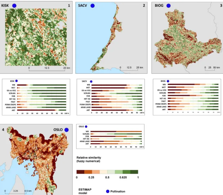
Fig. 2.(A and B): FN maps displaying spatial agreement between locally adapted ESTIMAP recreation models and their corresponding continental scale models. Slider diagrams in the lower panels depict relative correspondences between maps, grouped by land cover categories: WB = Water bodies; WET = Wetlands; OS no VEG = Open spaces with little or no vegetation; SCRUBS = Scrub and/or herbaceous vegetation; FOR = Forest; HET AG = Heterogeneous agricultural areas; PAST = Pastures; PERM CROPS = Permanent crops; ARAB LAND = Arable land; ART = Artificial.
The FN index among cases at the 100 m resolution were compa- rable across the three ES models. ESTIMAP pollination (mean ± s.d.
= 0.46 ± 0.17), was lower than both ESTIMAP recreation (0.53 ± 0.
15) and ESTIMAP air quality (0.62 ± 0.10). Spatial agreement between locally adapted models and their corresponding continen- tal models decreased with increasing levels of adaptation (F2,9= 4.26, P= 0.04). Models such as SIBB recreation and BARC recre- ation, which involved little amounts of adaptation (Table 1), had some of the highest FN indexes (Table 5). In contrast, local models that featured the largest amounts of adaptation, such as TRNA and KISK recreation models and the OSLO pollination model, had com- paratively low spatial agreement with their continental counter- parts (Table 5).
The TRNA, CNPM, and LLEV recreation models and the KISK, SACV and OSLO pollination models had high proportions of pixels with diverging predictions from the continental ESTIMAP models (Table 5). However, we found no consistent patterns between spa- tial agreement and the fragmentation of pixels with opposing
model predictions. The KISK pollination model, for example, had the highest proportion of pixels where SIP <0, together with a degree of fragmentation that was lower than many of the other models with comparable proportions of pixels with negative SIP values.
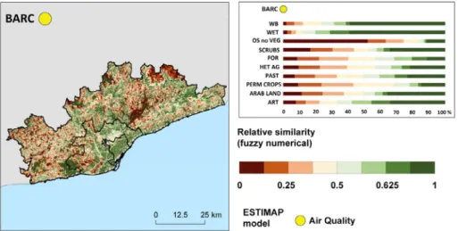
Cross tabulation of FN maps with dominant land use types revealed that one land cover category in particular exhibited extremely low spatial agreement with continental scale models (Figs. 2–4). For all recreation and pollination models, over half of all artificial land cover pixels had FN values <0.5. The arable land category also had large proportions of low FN values in some mod- els (see SIBB, CNPM and KISK recreation models, as well as SACV and OSLO pollination models), while other models showed quite high spatial agreement (BARC, TRNA and LLEV recreation models).
The categories of open space with no vegetation, forests and scrub and water bodies showed similar patterns with high spatial agree- ment in some models and comparatively low spatial agreement in others.
Fig. 3.FN maps displaying spatial agreement between locally adapted ESTIMAP pollination models and their corresponding continental scale models. Slider diagrams in the lower panels depict relative correspondences between maps, grouped by land cover categories: WB = Water bodies; WET = Wetlands; OS no VEG = Open spaces with little or no vegetation; SCRUBS = Scrub and/or herbaceous vegetation; FOR = Forest; HET AG = Heterogeneous agricultural areas; PAST = Pastures; PERM CROPS = Permanent crops;
ARAB LAND = Arable land; ART = Artificial.
3.3. Stakeholders’ opinions
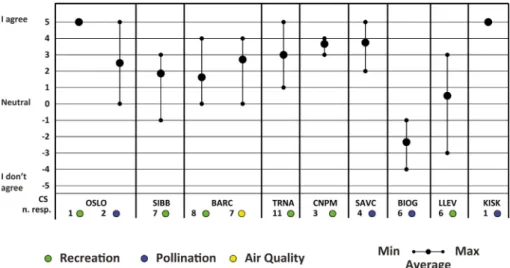
We received feedback from 49 individuals providing impres- sions of the ESTIMAP modelling process among the 246 question- naires collected from stakeholders and practitioners involved in all OpenNESS project case studies (Dick et al., 2018). Although four case studies used more than one ESTIMAP model, respondents from the KISK and SAVC cases only provided feedback regarding the pollination model. Stakeholders from cases that used ESTIMAP models reported low levels of their involvement in framing case studies’ research objectives and methodology. Mean scores for each case corresponded to ‘‘neutral” or less, although the range in scores suggest that certain individuals were more involved in the BARC, TRNA and CNPM cases (Fig. 5).
Stakeholders generally found the models relatively easy to understand and considered the assumptions underlying the meth- ods clear (Fig. 6, upper panel). However, stakeholders’ understand- ing varied both within and among groups. Stakeholder in the BARC and SIBB cases, for example, provided some of the lowest scores for model credibility. One respondent from BARC declared:
‘‘. . . The resulting map (ESTIMAP-recreation) looks like a map of
protected natural areas. The existence of recreational facilities, such
as picnic areas, itineraries, etc. outside protected areas can have a higher weight in terms of recreational use than the protection of a par- ticular area. Maybe data on these features is not available for all the case study area, but I think that some elements could be incorporated (important itineraries, trails, etc.)”
Stakeholders indicated that the need for technical assistance with applying ESTIMAP constituted a considerable constraint (Fig. 6, lower panel). The KISK case study was the only example where stakeholders expressed strong concerns that data availabil- ity constituted a constraint. Stakeholder opinion of the ESTIMAP’s model usability varied between the two extremes (Fig. 7). While many stakeholders provided largely positive feedback, at least some individuals in many cases had low opinions on how easy the model was to use or communicate to others. The mean scores for each case indicate that stakeholders’ overall impressions of ESTIMAP’s usefulness were predominantly positive (Fig. 8). Only the BIOG case had mean scores that reflected negative perceptions of the model’s utility.
Stakeholder comments provided additional depth for interpret- ing numerical assessment of the ESTIMAP modelling approach. Of the 111 comments stakeholders provided, we received 74 com- ments with content amenable to analysis. Most comments (70 %) Fig. 5.Index of participation in the OpenNESS case studies involving ESTIMAP. The index varies between 6 (deeply involved in the framing of the issue and selection of the tool) and – 6 (not involved) and depend on answers to Section 1, questions 1, 2, 3 (seeDick et al., 2018).
Fig. 4.FN maps displaying spatial agreement between locally adapted ESTIMAP air quality regulation model and their corresponding continental scale model. Slider diagrams in the lower panels depict relative correspondences between maps, grouped by land cover categories: WB = Water bodies; WET = Wetlands; OS no VEG = Open spaces with little or no vegetation; SCRUBS = Scrub and/or herbaceous vegetation; FOR = Forest; HET AG = Heterogeneous agricultural areas; PAST = Pastures; PERM CROPS = Permanent crops; ARAB LAND = Arable land; ART = Artificial.
addressed the models’ constraints, whereas the remaining 30%
related to usability (Fig. 9). Some examples of comments pertain- ing to models’ utility included the following narratives:‘‘. . .in par- ticular encouraged a great deal of discussion.”; ‘‘This was a very interesting tool in understanding land use around Loch Leven and assessing possible future tourism / recreational opportunities going forward.”; ‘‘Maps are highly useful for discussion. Visual tools to see differences across landscape. Useful for targeting – urban acupunc- ture.” ‘‘The maps and accompanying data was very interesting and easily understood so can help manage land and people. A good way to view whole park not so sure it’s as useful for the smaller areas as I think the managers will know their places”.
Stakeholders most frequently cited the complexity of the mod- els as a potential constraint. Examples of other comments address- ing ESTIMAP’s limitations pertained to difficulties in selecting the correct or most relevant scale (e.g., ‘‘The other thing was, not enough emphasis was put on the use of the surrounding hill for leisure activ- ities. Maps were good, but simplify too much”). Numerous respon- dents also expressed the problem in the ‘‘cartographic
consistency” of ESTIMAP output maps. The UK ordinance survey expresses the purpose of cartographic consistency as providing‘‘a map with balance. It enables features to be perceived as being organ- ised into groups and it allows maps themselves to belong to a family of products through a shared identity” (UK ordinance survey). Finally, we received one comment from a stakeholder who expressed con- cerns that the ESTIMAP tools were developed and explained in English.
4. Discussion
The examples from the OpenNESS case studies presented here provide insight into how context—the relevant decisions, spatial extent, stakeholder engagement, data precision and accuracy—de- termine model structure for mapping ES. Inspired by this work, we generated a conceptual diagram illustrating the key elements of a research agenda for ES modeling (Fig. 10). The primary user group of any map defines the spatial extent for the mapping exercise Fig. 6.Stakeholder perceptions of applying ESTIMAP models to local contexts, in response to questions addressing their understanding of methods and results (upper) and the methods’ constraints (lower).
(vertical axis). The needs of the users for decision support and the intended policy or management application will define both the resolution necessary to capture the relevant spatial heterogeneity (depth axis) and the necessary levels of information accuracy (hor- izontal axis). The costs of acquiring and producing information will increase with increasing spatial extent, spatial resolution and accu- racy requirements. The considerable recent advances in remote sensing’s accessibility has made large-scale, high-resolution map- ping possible for representing ecosystems’ extent and even condi- tion (de Araujo Barbosa et al., 2015; Galbraith et al., 2015;
Rocchini, 2015), effectively reducing the cost of many aspects of ES mapping. However, these cost savings may not necessarily affect the costs associated with increasing model accuracy. We contend that increases in model accuracy—or models’ ultimate utility—can best be achieved through the process of knowledge co-production, where experts, stakeholders and other users/bene- ficiaries actively participate in relating the available spatial data to the appropriate measurements of ES for a given purpose.
Exploring multiple ESTIMAP model adaptations within a broader research project provides some interesting insight into
model adaptation and the importance of determining the model’s policy or management related purpose at an early stage.Harrison et al. (2018)investigated what criteria OpenNESS case studies used for selecting the mapping and analytical methods used in their case, and identified four non-exclusive approaches. Method selec- tion was methods-oriented if case study teams chose methods based on whether the data, expertise or resources needed to apply the methods were available. Methods selection was research- oriented if case study teams considered the method useful for cov- ering research gaps or if researchers intended to apply the methods to make comparisons across cases. Method selection was stakeholder-oriented if the study outcomes could encourage stake- holder dialog and deliberation, or if stakeholders were involved in the co-production of knowledge. Methods selection was decision- oriented if the outcomes were important to inform spatial planning or evaluate policies.
All case studies that used ESTIMAP models were either moder- ately or strongly research- and methods-oriented (Harrison et al., 2018). Comparatively few were equally stakeholder- or decision- oriented, a finding that stakeholder responses to questionnaires Fig. 7.Stakeholder perceptions of applying ESTIMAP models to local contexts, in response to questions addressing method’s usability.
Fig. 10.Conceptual diagram of how ES mapping may vary according to spatial extent, spatial resolution (or spatial precision) and informational reliability—ultimately determining the costs of producing information (red axes). With increased stakeholder involvement, mapping moves to knowledge co-production. Adapted fromGómez- Baggethun and Barton (2013).
Fig. 8.Case study stakeholder’s impression of the overall usefulness of ESTIMAP models for addressing local ecosystem service mapping needs.
Fig. 9.Classification of 77 comments provided by case study stakeholders regarding using ESTIMAP models for local ecosystem service mapping contexts. Squares area is proportional to the frequency of themes and sub-themes.
confirmed. As a possible consequence of the emphasis on methods or research, very few cases had clearly defined the relevant policy questions before the modelling work began. As work progressed, research teams also worked to find and apply data at the highest available resolution—irrespective of which spatial resolution was most appropriate because the decision context had yet to be defined. This manner of progression may explain some stakehold- ers’ dissatisfaction with model believability, ease of use or ease of communication. Stakeholder attitudes regarding ESTIMAP’s com- plexity reinforce our sense that future use of these models will continue to require assistance of a research team. Creating a user toolbox to facilitate public use of ESTIMAP was not an objective of the OpenNESS project.
With a clearly defined decision context, determining the spatial extent of an ES spatial model is reasonably straightforward. The local adaptations of ESTIMAP involved mapping at extents that ranged from 84 to 4500 km2. These extents constituted scales of relevance from the property to regional levels and corresponded with end users that ranged from property owners to local govern- ments (Fig. 10). The spatial extent will at least partially dictate the spatial resolution. However, adaptation of a spatial model to local contexts is not just a matter of acquiring data with the highest pos- sible spatial resolution for a given spatial extent. What is more important is utilizing a spatial resolution that is sufficient for cap- turing the spatial heterogeneity that is relevant to variation in ES supply.
We use precision differential as a measure of the spatial agree- ment between comparable models at different spatial scales and model structures. It is important to note that precision differential values do not constitute a measure of model accuracy or reliability.
Assessing accuracy would require obtaining repeated observations or using independent datasets generated from other methods—
measures described inFig. 10as ‘‘reliability costs” (also referred to as ground-truthing). ES mapping is a relatively new field, and the reliability of the information it produces may be limited as the field matures. Developing and accumulating external data sets for model validation and repeated mapping over time will ulti- mately allow decision-makers and researchers to assess ES spatial model reliability.
Precision differential metrics provide a way of assessing both how and where spatial scales and model structure produce models with contrasting outputs. In OpenNESS case study applications of ESTIMAP models, we found no systematic patterns that would sug- gest that precision varies with the ES of the model, nor did we find that precision differential scores vary according to the spatial
extent. What is clear, however, was that land cover categories can vary considerably in their ability to capture relevant hetero- geneity at larger spatial scales. Areas with systematically low FN or negative SIP values require extra attention when downscaling ES spatial models. In particular, artificial land cover had high pro- portions of pixels with low spatial agreement between correspond- ing models for both recreation and pollination. Areas classified as artificial land cover at low spatial resolutions include considerable spatial heterogeneity relevant to the potential ES supply. Since artificial land cover is an important part of urban areas, knowledge co-design can be particularly important to identify which elements are important for mapping of urban ES, and what spatial scale is appropriate.
Specific details from the local adaptations of two case studies’
ESTIMAP models help illustrate the value of dialogue with stake- holders and the model end users. The Loch Leven recreation model was adapted to explore the recreation potential in and around the lake. Whereas European scale mapping of recreation potential lim- its its consideration of water elements in terms of presence, water qualityis a major determinant of the recreational opportunities in and around Loch Leven. Harmful algal blooms (HABs) are a specific concern there (Carvalho et al., 2012) and can both adversely affect recreational fishing and limit other leisure activities along the lake path, such as dog walking. Yet despite increased monitoring of European water quality driven by the Water Framework Directive (Directive 2000/60/EC, 2000), suitable water quality data are avail- able for only a small fraction of European surface waters. The case study team managed to overcome this limitation by modelling recreational risks from HABs by using estimated nutrient concen- trations of European lakes in combination with published statisti- cal models linking nutrient status to HAB (Carvalho et al., 2013).
Experience garnered from using ESTIMAP at the Loch Leven case may have broader implications for modelling water-related recre- ation at either other similar sites or larger spatial scales. Modelling recreational potential around waters and the importance of water quality in shaping that potential, is very relevant to implementa- tion of water policy in Europe. Outputs from the model can be used to support and supplement WFD implementation by emphasizing the social and economic benefits of achieving good ecological sta- tus, providing a stronger case for justifying the costs of restoring aquatic ecosystems (Grizzetti et al., 2016).
The OSLO pollination model is another example of an ESTIMAP model that underwent major modifications to fit the local biophys- ical conditions and the management context. The intended pur- pose of the continental scale ESTIMAP model was to describe
Table 6
Protocol for adapting ESTIMAP models to a local context.
Step Sub steps Description
1. Define the type of knowledge production (or co-production) – and the uses of the new information created
Define the applications of the analysis
Clarify what decision context (which type of policy / planning or managing actions) will be informed by the model
Define the final map users Clarify who will use the final results of the models, and what skills or guidance they might need to interpret output maps
Chose which stakeholders (SH) to engage
Define which level of stakeholder involvement will be possible or most useful: either simple consultation or real co-production as a part of an interactive process
2. Choose the scale(s) of the analysis (temporal and Spatial scale)
Clarify whether decision context needs a temporal analysis or a scenario assessment.
Define if different time series are needed (this will affect the spatial extent (s) as well as the data availability and preparation)
Determine the spatial extent(s) Define the scale of management, production, use of the ES Positional Absolute Accuracy Define the precision of the data sets
Attribute and scoring accuracy Describe how each input data and component was scored 3. Build the conceptual schema of the model Definition of model rules
(components, combination logic, scoring system, weights)
Starting from the conceptual schema proposed for the EU scale application define: 1) number of components; 2) combination of inputs, 3) type of scoring system, 4) presence of weighing parameters
4. Include and prepare the data The type of data and the preparation process is strongly related to step 1, 2, and 3
5. Run model and share results Get user feedback on model outputs, and explore options for verifying ES maps with independent data. If necessary, refine model structure (Step 3).