International Integration
T
An empirical analysis on volatility:
Evidence for the Budapest
stock exchange using GARCH model
NGO THAI HUNG
Corvinus University of Budapest
Submitted: March 27, 2017 – Accepted: May 25, 2017
Abstract:
he paper aims to analyze and forecast the Budapest Stock Exchange volatility with the use of generalized autoregressive conditional heteroscedasticity GARCH- type models over the time period from September 06, 2010 to March 03, 2017. This model is the extension of ARCH process with various features to explain the obvious characteristics of financial time series such as asymmetric and leverage effect. As we apply the Budapest Stock Exchange with this model, the estimation and forecast in short term are performed.
Keywords: Volatility, GARCH, BUX, Volatility forecast.
1. Introduction
In recent years, the study of the volatility of a market variable measuring uncertainty about the future value of the variable plays a prominent part in monitoring and assessing potential losses.
Quantitative methods measure the volatility of the Budapest Stock Exchange BUX received the high interest because of its role in determining the price of securities and risk management. Typically, a series of financial indices have different movements under certain period. This means that the variance of the range of financial indicators changes over time. The Budapest Stock Exchange is one of the most crucial markets by market capitalization and liquidity in central Europe. BUX accounts for all the turnover in Hungarian market and a large share of the Central and Easter Europe market.
According to Bank (2015), the fundamental economic role of the Budapest Stock Exchange is to provide the domestic enterprises with an opportunity to raise capital. In recent years, the domestic capital market has fulfilled this role. At present, the demand side of the stock exchange is dominated by non-resident institutions. Therefore,
the investigation of the volatility of the Budapest Stock Exchange is in need.
As Bantwa (2017) mentioned, for most investors, the prevailing market turmoil and lack of clarity on where it's headed are a cause for concern. The majority of investors in markets are mainly concerned about the uncertainty in getting the expected returns as well as the volatility in returns.
Andersen T. and Labys (2003) provided a framework for integrating high-frequency intraday data into the measurement, modelling, and forecasting of daily and lower frequency return volatilities and return distributions. Use of realized volatility computed from high-frequency intraday returns permits used of traditional time series methods for modelling and calculating.
Ashok and Ritesh (2011) center on comparing the performance of conditional volatility model GARCH and Volatility Index in predicting underlying volatility of the NIFTY 50 index. Using high-frequency data the underlying volatility of NIFTY50 index is captured. Several approaches to predicting realized volatility are considered.
International Integration
270
Chatayan Wiphatthanananthakul (2010) estimated ARMA-GARCH, EGARCH, GJR and PGARCH models for Thailand Volatility Index (TVIX), and made comparison and forecast between the models.GARCH model has become key tools in the analysis of time series data, particularly in financial applications. This model is especially useful when the goal of the study is to analyse and forecast volatility Degiannakis (2004). With the generation of GARCH models, it is able to reproduce another very vital stylized fact, which is volatility clustering; that is, big shocks are followed by big shocks.
In this paper, we applied GARCH model to estimate, compute and forecast the Budapest Stock Exchange volatility. Nevertheless, it should be pointed out that several empirical studies have already examined the impact of asymmetries on the performance of GARCH models. The recent survey by Poon and Granger (2003) provides, among other things, an interesting and extensive synopsis of them. Indeed, different conclusions have been drawn from these studies. The rest of the paper proceeds as follows: the concept of volatility and GARCH model are given in next section, the final section is discussed results and conclusion.
2. Theoretical Background, Concept and Definitions
• Definition and Concept of Volatility
The volatility of a variable is defined as the standard deviation of the return provided by the variable per unit of time when the return is expressed using continuous compounding. When volatility is used for option pricing, the unit of time is usually one year, so that volatility is the standard deviation of the continuously compounded return per year. However, when volatility is used for risk management, the unit of time is usually one day, so that volatility is the standard deviation of the continuously compounded return per day.
In general, T is equal to the standard deviation of
0
ln ST S
where ST is the value of the market variable at time T and S0 is its value today. The
expression
0
ln ST S
equals the total return earned in time T expressed with continuous compounding.
If is per day, T is measured in days, if is per year, T is measured in years, according to C.Hull (2015).
The volatility of EUR/HUF variable is estimated using historical data. The returns of EUR/HUF at time t are calculated as follows:
1
ln i , 1,
i
i
R p i n
p
where pi and pi1 are the prices of EUR/HUF at time t and t-1, respectively. The usual estimates s of the standard deviation of the Riis given by
2 1
1 ( )
1
n i i
s R R
n
where Ris the mean of the Ri.
As explained above, the standard deviation of the Ri is T where is the volatility of the EUR/HUF.
The variable s is, therefore, an estimate of T . It follows that itself can be estimated as ˆ, where
ˆ s
T
The standard error of this estimate can be shown to be approximate ˆ
2n
. T is measured in days, the
volatility that is calculated is a daily volatility.
• GARCH Model
GARCH model by Bollerslev(1986) imposes important limitations, not to capture a positive or negative sign of ut, which both positive and
International Integration
negative shocks have the same impact on the conditional variance, ht, as follows
t t t
u
2 2 2
1
1 1
p q
t i t j t j
i j
u
where 0, 10, for i1,p and j 0 for 1,
j q are sufficient to ensure that the conditional variance, t is nonnegative.
For the GARCH process to be defined, it is required that 0. Additionally, a univariate GARCH(1,1) model is known as ARCH() model Engle, (1982) as an infinite expansion in ut21. The
represents the ARCH effect and represents the GARCH effect. GARCH(1,1) model, t2 is calculated from a long run average variance rate, VL, as well as from
t1 and ut1. The equation for GARCH(1,1) is2 2 2
1 1
t VL ut t
where is the weight assigned to VL, is the weight assigned to ut21 and is the weight assigned to t21. Since the weight must sum to one, we have
1
• Volatility forecasting
There is a vast and relatively new literature that attempts to compare the accuracies of various models for producing out-of-sample volatility forecasts. Akgiray (1989), for example, finds the GARCH model superior to ARCH, exponentially weighted moving average and historical mean models for forecasting monthly US stock index volatility.
A similar result concerning the apparent superiority of GARCH is observed by West and Cho (1995) using one-step-ahead forecasts of dollar exchange rate volatility, although for longer horizons, the model behaves no better than their alternatives.
A particularly clear example of the style and content of this class of research is given by Day and Lewis (1992). The Day and Lewis study will therefore now be examined in depth. The purpose of their paper is to consider the out-of-sample forecasting performance of GARCH and EGARCH models for predicting stock index volatility.
Arowolo, W.B employed the properties of linear GARCH model for daily closing stocks prices of Zenith bank PlC in Nigeria stocks Exchange, they concluded that the Optimal values of p and q GARCH (p,q) model depends on location, the types of the data and model order selected techniques being used. The models that Day and Lewis employ so called a ‘plain vanilla’
GARCH(1,1):
2
0 1 1 1 1
t t t
h u h
• Data Description
The data for our empirical investigation consists of the Budapest Stock Exchange index transaction prices that is obtained from Bloomberg, accounted by the Department of Finance, Corvinus University of Budapest, the sample period is from September 06, 2010 to March 03, 2017 which constitutes a total of n = 1694 trading days. For the estimation, we use the daily returns of Budapest Stock Exchange index to estimate GARCH(1,1) by using Eview 7.0 software.
3. Results and discussion
• Descriptive Statistics
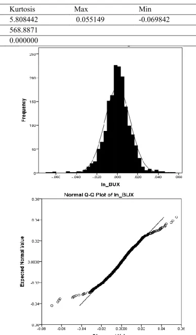
The descriptive statistics of daily logarithmic returns of the Budapest Stock Exchange index is given in Table 1.
International Integration
272
Table 1. Descriptive statistics of EUR/HUF Returns
Mean Std. Dev Skewness Kurtosis Max Min
0.000251 0.012509 -0.207632 5.808442 0.055149 -0.069842
Jarque-Bera 568.8871
Probability 0.000000
Source: Author’s calculation
The average return of BUX is positive. A variable has a normal distribution if its skewness statistic equals to zero and kurtosis statistic is 3, but the return of BUX has negative skewness statistic and high kurtosis, suggesting the presence of fat tails and a non-symmetric series. Additionally, as we can see from Jarque-Bera normality test rejects the null hypothesis of normality for the sample, this means we can draw a conclusion that the return of BUX is not normally distributed. The relatively large kurtosis indicates non-normality that the distribution of returns is leptokurtic.
Figure 1 depicts the histogram of daily logarithmic return for BUX. From this histogram, it appears that BUX returns have high peak than the normal distribution. In general, Q-Q plot is used to identify the distribution of the sample in the study, it compares the distribution with the normal distribution and indicates that BUX returns deviate from the normal distribution.
Figure 1. Histogram and Q-Q Plot of Daily Logarithmic BUX returns
12,000 16,000 20,000 24,000 28,000 32,000 36,000
2010 2011 2012 2013 2014 2015 2016
BUX
International Integration
-.08 -.06 -.04 -.02 .00 .02 .04 .06
2010 2011 2012 2013 2014 2015 2016
LN_BUX
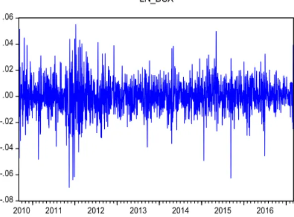
Figure 2. Daily price and BUX returns
The unit root tests for BUX returns are summarized in Table 2. The Augmented Dickey-Fuller (ADF) and Phillips-Perron (PP) tests were used to test the null hypothesis of a unit root against the alternative hypothesis of stationarity. The tests have large negative values of statistics in all cases for levels such that the return variable rejects the null hypothesis at the 1 per cent significance level, therefore, the returns are stationar
Figure 2 presents the plot of price and BUX returns. This indicates some circumstances where BUX returns fluctuate.
Table 2. Unit root test for Returns of EUR/HUF
Test None Constant Const & Trend
Phillips-Perron -40.95554 -40.96258 -41.02295
ADF -40.92542 -40.93358 -40.98122
Source: Author’s calculation
• Estimation
Table 3 represents the ARCH and GARCH effects from statistically significant at 1 percent level of
and . It shows that the long-run coefficients are all statistically significant in the variance equation. The coefficient of appears to show the
presence of volatility clustering in the models.
Conditional volatility for the models tends to rise (fall) when the absolute value of the standardized residuals is larger (smaller). The coefficients of (a determinant of the degree of persistence) for all models are less than 1 showing persistent volatility.
Table 3. GARCH on Returns of BUX GARCH
Mean Equation Variance Equation
Coefficient z-statistics Coefficient z-statistics
Constant 0.000518 1.885713 0.0000064 5.277486
(0.0000)
Mean 0.086160 7.033843
(0.0000)
0.871707 50.44310
(0.0000) Source: Author’s calculation
GARCH (1,1) model is estimated from daily data as follows
2 2 2
1 1
0.0000064 0.086160 0.871707
t ut t
Since 1 , it follows that 0,042133 and, since VL. We have VL 0,000159. In
other words, the long run average variance per day implied by the model is 0,000159. This corresponds to a volatility of
0,000159 0.0123 or 1.23 %, per day.
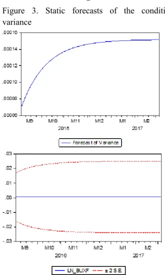
• Forecasting Results Using GARCH (1,1) Model
The selected model
International Integration
274
2 2 2
1 1
0.0000064 0.086160 0.871707
t ut t
has been tested for diagnostic checking and there is no doubt of its accuracy for forecasting based on residual tests. We can use our model to predict the future volatility value. Figures 3 and 4 show the forecast value. It is seen that the forecasts of the conditional variance indicate a gradual increase in the volatility of the stock returns. The dynamic forecasts show a completely flat forecast structure for the mean, while at the end of the in-sample estimation period, the value of the conditional variance was at a historically low level relative to its unconditional average. Therefore, the forecast converges upon their long term mean value from below as the forecast horizon increases. Notice also that there are no 2-standard error band confidence intervals for the conditional variance forecasts. It is evidence for, static forecasts that the variance forecasts gradually go up the out–of sample period, they show much more volatility than for the dynamic forecasts.
Figure 3. Static forecasts of the conditional variance
Figure 4. Dynamic forecasts of the conditional variance
Conclusions
This paper estimates the volatility of the Budapest Stock Exchange returns using GARCH model from the seemingly complicated volatility formula established by Bollerslev (1986). The results of statistical properties obtained supported the claim that the financial data are leptokurtic. The GARCH model was identified to be the most appropriate for the time-varying volatility of the data. The results from an empirical analysis based on the Budapest Stock Exchange showed the volatility is 1.23 % per day. Additionally, the results of forecasting conditional variance indicate a gradual increase in the volatility of the stock returns. This is in contrast to the work of Chatayan Wiphatthanananthakul (2010).
International Integration
References
Akgiray, V. (1989) Conditional Heteroskedasticity in Time Series of Stock Returns:
Evidence and Forecasts, Journal of Business 62(1), 55—80
Arowolo, W.B (2013), Predicting Stock Prices Returns Using GARCH Model, The International
Ashok Bantwa (2017). A study on India volatility index (VIX) and its performance as risk management tool in Indian Stock Market. Indian Journal of Research, 06:248, 251.
Banerjee Ashok and Kumar Ritesh (2011). Realized Volatility and India VIX, IIM Calcutta.
Working Paper Series, (688).
Bank, M. N. (2015). Budapest Stock Exchange is once again in Hungarian hands. retrieved from:
https://www.mnb.hu/en/pressroom/press- releases/press-releases-2015/budapest-stock- exchange-is-once-again-in-hungarian-hands Chatayan Wiphatthanananthakul and Songsak
Sriboonchitta (2010), The Comparison among ARMA-GARCH, -EGARCH, -GJR, and - PGARCH models on Thailand Volatility Index, The Thailand Econometrics Society, Vol. 2, No. 2, 140 - 148
Day, T. E. and Lewis, C. M. (1992) Stock Market Volatility and the Information Content of
Stock Index Options, Journal of Econometrics 52, 267—87 Diebold F.X. Andersen T., Bollerslev T. and P. Labys
(2003). Modelling and Forecasting
Realized Volatility. Econometrica, 71:529, 626.
John C.Hull (2015). Risk management and Financial Institutions, volume 4. John Wiley &
Sons, Inc., Hoboken, New Jersey.
S. H. Poon and C. W. J. Granger (2003). Forecasting volatility in financial markets: A
review. Journal of Economic Literature, 41:478, 539.
Stavros Degiannakis (2004). Forecasting realized intraday volatility and value at Risk:
Evidence from a fractional integrated asymmetric Power ARCH Skewed t model. Applied Financial Economics.
T. Bollerslev.(1986). Generalized autoregressive heteroskedasticity. Journal of Econometrics, 31:307, 327, 1986.
West, K. D. and Cho, D. (1995). The Predictive Ability of Several Models of Exchange Rate Volatility, Journal of Econometrics 69, 367—91. Journal of Engineering and Science, volume 2, 32-37
Nghiên Cứu & Trao Đổi International Integration
APPENDIX Residual test
Date: 03/20/17 Time: 10:05 Sample: 9/07/2010
3/03/2017
Auto correlation
Partial
Correlation AC PAC Q-Stat Prob
Included observations: 1694 | | | | 18 0.021 0.019 20.942 0.282
| | | | 19 -0.034 -0.038 22.915 0.241 Auto
correlation
Partial
Correlation AC PAC Q-Stat Prob | | | | 20 -0.005 -0.012 22.950 0.291
| | | | 21 0.053 0.057 27.865 0.144
| | | | 1 0.014 0.014 0.3274 0.567
| | | | 2 -0.000 -0.001 0.3277 0.849
| | | | 3 -0.028 -0.028 1.6194 0.655
| | | | 4 0.020 0.021 2.2997 0.681
| | | | 5 -0.050 -0.051 6.5817 0.254
| | | | 6 0.004 0.005 6.6124 0.358
| | | | 7 -0.006 -0.005 6.6720 0.464
| | | | 8 -0.000 -0.003 6.6722 0.572
| | | | 9 0.039 0.042 9.3182 0.408
| | | | 10 0.048 0.044 13.252 0.210
| | | | 11 0.001 0.001 13.255 0.277
| | | | 12 0.007 0.008 13.328 0.346
| | | | 13 0.012 0.012 13.554 0.406
| | | | 14 -0.020 -0.018 14.211 0.434
| | | | 15 -0.058 -0.053 19.883 0.176
| | | | 16 0.007 0.009 19.970 0.222
| | | | 17 -0.011 -0.012 20.176 0.265
| | | | 22 0.046 0.039 31.470 0.087
| | | | 23 -0.018 -0.015 31.999 0.100
| | | | 24 -0.022 -0.016 32.858 0.107
| | | | 25 0.024 0.029 33.853 0.111
| | | | 26 -0.011 -0.009 34.055 0.134
| | | | 27 0.025 0.029 35.123 0.136
| | | | 28 -0.009 -0.007 35.256 0.163
| | | | 29 -0.003 -0.004 35.268 0.196
| | | | 30 -0.034 -0.036 37.232 0.170
| | | | 31 0.039 0.030 39.873 0.132
| | | | 32 -0.028 -0.029 41.251 0.127
| | | | 33 0.025 0.027 42.308 0.129
| | | | 34 -0.007 -0.012 42.403 0.153
| | | | 35 -0.001 -0.007 42.404 0.182
| | | | 36 -0.011 0.001 42.630 0.207
400 350 300 250 200 150 100 50 0
Series: Standardized Residuals Sample 9/07/2010 3/03/2017 Observations 1694
Mean -0.026025 Median -0.019700 Maximum 3.669658 Minimum -6.335468 Std. Dev. 0.999052 Skewness -0.267553 Kurtosis 4.909524 Jarque-Bera 277.5775 Probability 0.000000
274
PHÁT TRIỂN & HỘI NHẬP Số 35 (45) - Tháng 07 - 08/2017Nghiên Cứu & Trao Đổi Bilingualism and its economic
advantages
(Continued from p.268)
RefeReNces
Heteroskedasticity Test: ARCH
F-statistic 0.025406 Prob. F(1,1691) 0.8734
Obs*R-squared 0.025436 Prob. Chi-Square(1) 0.8733
Test Equation:
Dependent Variable: WGT_RESID^2 Method: Least Squares
Date: 03/20/17 Time: 10:07
Sample (adjusted): 9/08/2010 3/03/2017 Included observations: 1693 after adjustments
Variable Coefficient Std. Error t-Statistic Prob.
C 1.001428 0.053938 18.56623 0.0000
WGT_RESID^2(-1) -0.003876 0.024318 -0.159392 0.8734
R-squared 0.000015 Mean dependent var 0.997556 Adjusted R-squared -0.000576 S.D. dependent var 1.981039 S.E. of regression 1.981610 Akaike info criterion 4.206877 Sum squared resid 6640.181 Schwarz criterion 4.213296 Log likelihood -3559.121 Hannan-Quinn criter. 4.209254 F-statistic 0.025406 Durbin-Watson stat 1.999504 Prob(F-statistic) 0.873379
Baker, C. (1988). Key issues in bilingualism and bilingual education. Clevedon: Multilingual Matters.
Bialystok, E. (2001). Bilingualism in development:
Language, literacy, and cognition. Cambridge:
Cambridge University Press.
Bloomfield, L. (1933). Language. New York: Holt.
Devlin, K. (2015, July). Learning a foreign language a ‘must’ in Europe, not so in America. Retrieved from Pew Research Center website: http://www.
pewresearch.org/fact-tank/2015/07/13/learning- a-foreign-language-a-must-in-europe-not-so-in- america/
Döpke, S. (1992). One parent–one language: an interactional approach. Amsterdam: Benjamins.
Edwards, J. (2010). Language diversity in the classroom. Great Britain: the Cromwell Press Group.
Grosjean, F. (1989). Neurolinguists, beware! The bilingual is not two monolinguals in one person.
Brain and Language, 36, 3-15.
Haugen, E. (1953). The Norwegian language in America. Philadelphia, PA: University of Pennsylvania Press.
Porras, D., Ee, J., & Gándara, P. (2014). Employer preferences: Do bilingual applicants and employees experience an advantage? In R. Callahan & P.
Gándara (Eds.), The bilingual advantage language, literacy and the US labor market (pp. 236-262).
Clevedon, UK: Multilingual Matters.
Stone, R. (2011, Sep). Reducing the impact of language barriers (Executive Report from Forbes Insights).
Retrieved from Forbes Insights Archives: http://
resources.rosettastone.com/CDN/us/pdfs/Biz- Public-Sec/Forbes-Insights-Reducing-the-Impact- of-Language-Barriers.pdf
U.S. Census Bureau. (2013). Language use in the United States: 2011. Retrieved from www.census.
gov/prod/2013pubs/acs-22.pdf
Wai Yin Pryke. (2014). Singapore’s Journey:
Bilingualism and role of English language in our development [PowerPoint slides]. Retrieved from https://www.britishcouncil.cl/sites/default/files/
powerpoint-wai-yin-pryke.pdf Số 35 (45) - Tháng 07 - 08/2017 PHÁT TRIỂN & HỘI NHẬP