Multicriteria Decision Making and Rankings Based on Aggregation Operators
(Application on Assessment of Public Universities and Their Faculties)
Lucia Vavríková
Department of Mathematics, Faculty of Civil Engineering, Slovak University of Technology
Radlinského 11, 813 68 Bratislava, Slovakia vavrikova@math.sk
Abstract: In order to solve decision making problem we have to compare and rank a finite set of alternatives. In this paper we want to show some approaches to creating the preference structure (ranking) of alternatives. These approaches lead us to use chosen multicriteria decision methods and aggregation operators. ARRA (Academic ranking and rating agency) uses one fixed way to create a ranking of public universities and their faculties. In this paper many more approaches to creating such rankings (or preference structures) of alternatives are discussed and the results are compared.
Keywords: Alternative; preference structure; multicriteria method; aggregation operator
1 Introduction
ARRA (Academic ranking and rating agency) publishes every year an assessment report concerning public universities and their faculties. The higher education institution assessment procedure consists of the following steps:
• the selection of indicators (criteria) for the quality of education and research in individual universities and the assignment of a certain number of points to each faculty for the performance in the particular indicator (indicators are arranged into groups and each group of indicators gains a certain number of points),
• the partition of faculties into six groups according to the so-called Frascati Manual in order to compare only faculties that have the same orientation and similar working conditions,
• assigning a point score to faculties (the ranking is based on the average points score in the individual groups of indicators),
• calculating the point scores for the higher education institutions in individual Frascati groups (the ranking of the institution in the given group is given by the average assessment of all its faculties included in that group). For more details, see [8].
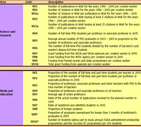
Assessment criteria created by ARRA [8] are shown in the table below.
Table 1 Criteria created by ARRA
For simplicity in the examples we have chosen seven faculties (alternatives) ai, i=1,…,7 (from a total number of 24 technical specialized faculties evaluated by ARRA) and five evaluation criteria Cj, j=1,…,5, one from every set: SV1-SV4 ⇨ C1, SV6-SV8 ⇨ C2, VV1-VV3a ⇨ C3, VV4-VV6 ⇨ C4, VV7-VV10 ⇨ C5.
In the following examples the differences between the ARRA rankings (preference structures) and other ranking methods are shown.
Example 1
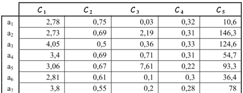
Take a set of alternatives A = (a1,…,a7). Every alternative ai is described by five criteria C1,…, C5 see table below.
Table 2 Input data
C 1 C 2 C 3 C 4 C 5
a1 2,78 0,75 0,03 0,32 10,6 a2 2,73 0,69 2,19 0,31 146,3 a3 4,05 0,5 0,36 0,33 124,6 a4 3,4 0,69 0,71 0,31 54,7 a5 3,06 0,67 7,61 0,22 93,3 a6 2,81 0,61 0,1 0,3 36,4 a7 3,8 0,55 0,2 0,28 78 Our aim is to create a final ranking on these alternatives.
2 The Basics of Preference Relations Notations
When the decision maker chooses between two alternatives (which are not incomparable) described by score vectors x and y within his choice set, he is able to say that he prefers x to y (or vice-versa) or he has the possibility to say that two alternatives are indifferent (equivalent). We will not distinguish alternative a and its corresponding score vector x.
• Strict preference (P) - a couple of alternatives x, y belongs to the relation P, if and only if the decision maker strictly prefers x to y (x P y): x ≻ y.
• Indifference (I) - a couple of alternatives x, y belongs to the relation I, if and only if the decision maker is indifferent between alternatives x and y (x I y): x ≈y.
• Incomparability (J) - a couple of alternatives x, y belongs to the relation J, if and only if the decision maker is unable to compare x and y (x J y).
(But this is not our case.)
3 Multicriterial Methods Used in the Assessment of Public Universities
In this section we recall three of the often used social choice procedures and their application on the assessment. Note that these methods are usually used in voting systems to find a winner, and they can be applied to create rankings, as well.
3.1 Borda Count Method
For the Borda Count Method, each candidate (alternative) gets 1 point for each last place vote received, 2 points for each next-to-last point vote, etc., all the way up to m points for each first place vote (where m is the number of candidates/alternatives). The candidate with the largest point total wins the election.
Bi = ij, i=1,2,...,n (1)
Bij is a number assigned by j-th expert (criterion) to i-th candidate (alternative).
The ranking is done using Bi as the utility function value for alternative (candidate) i.
3.2 Plurality Voting
The idea of plurality voting is simply to declare as the social choices the alternatives with the largest number of first-place rankings in the individual preference list. The successive application of the plurality voting method, omitting its actual winners, can serve for ranking purposes.
3.3 The Hare System
This system is based on the idea of arriving at a social choice by successive deletions of less desirable alternatives. If any alternative occurs at the top of at least half of the preference lists, then it is declared to be a social choice [7].
Ranking can be achieved by using a similar strategy as plurality voting.
Example 2
The preference structures by the criteria C j (see Table 1) are as follows:
C 1: a3 ≻a7≻ a4 ≻ a5≻a6≻a1≻ a2,
C 2: a1 ≻ a2 ≈ a4 ≻ a5≻a6≻a7≻ a3,
C 3: a5 ≻ a2≻ a4≻a3≻a7≻a6≻a1,
C 4: a3 ≻ a1≻ a2 ≈ a4≻a6≻a7≻a5,
C 5: a2 ≻ a3≻ a5≻a7≻a4≻a6≻a1.
The final preference structures via the usage of the mentioned methods are:
Borda count method (B.C.): a3 ≻a2 ≻ a4≻a5≻ a1≈ a7≻ a6.
Plurality voting (P.V.): a3 ≻a1 ≻ a2≻ a4 ≻ a5 ≻ a7 ≻ a6.
Hare system (H.S.): a3 ≻a1 ≻ a2≻ a4 ≻ a5 ≻ a7 ≻ a6.
These three methods satisfy monotonicity and the Pareto condition.
4 Linear Normalization of Input Data
Data normalization consists of rescaling the attribute values of the data into a single specified range, such as from 0 to 1 or from 0 to 100.
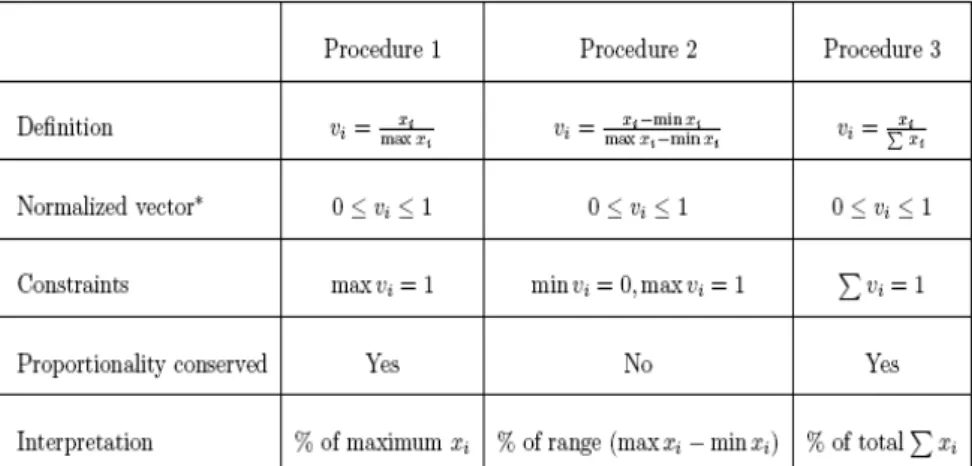
In the following table are shown 3 basic arithmetic processes of linear normalization.
Table 3 Linear normalization
Conditions under which the methods can be applied: xi ≥ 0,
x1,…,xn are the input values and the values v1,...,vn are normalized outputs.
* except for some pathological values of xi (if x1= … = xn, then the corresponding criterion C j gives no information and it can be omitted).
Example 3
We continue in Example 1, i.e., we consider Table 2. In the following tables we show the normalized inputs according to three different Procedures 1, 2, 3.
Table 4
Procedure 1 of linear normalization
C 1 C 2 C 3 C 4 C 5
a1 68,64 100,00 0,39 96,97 7,25 a2 67,41 92,00 28,78 93,94 100,00 a3 100,00 66,67 4,73 100,00 85,17 a4 83,95 92,00 9,33 93,94 37,39 a5 75,56 89,33 100,00 66,67 63,77 a6 69,38 81,33 1,31 90,91 24,88 a7 93,83 73,33 2,63 84,85 53,32
Table 5
Procedure 2 of linear normalization
C 1 C 2 C 3 C 4 C 5
a1 3,79 100,00 0,00 90,91 0,00 a2 0,00 76,00 28,50 81,82 100,00 a3 100,00 0,00 4,35 100,00 84,01 a4 50,76 76,00 8,97 81,82 32,50 a5 25,00 68,00 100,00 0,00 60,94 a6 6,06 44,00 0,92 72,73 19,01 a7 81,06 20,00 2,24 54,55 49,67
Table 6
Procedure 3 of linear normalization
C 1 C 2 C 3 C 4 C 5
a1 12,28 16,82 0,27 15,46 1,95 a2 12,06 15,47 19,55 14,98 26,90 a3 17,90 11,21 3,21 15,94 22,91 a4 15,02 15,47 6,34 14,98 10,06 a5 13,52 15,02 67,95 10,63 17,15 a6 12,42 13,68 0,89 14,49 6,69 a7 16,79 12,33 1,79 13,53 14,34 Remark 1
The linear normalization of input data saves the preferences between alternatives in individual criteria, but for different aggregation methods the final preference structures may be different.
5 Chosen Aggregation Operators
In many decision making problems, a number of independent attributes or criteria are often used to individually rate an alternative from the decision maker's perspective and then these individual ratings are combined to produce an overall assessment.
In decision making, values to be aggregated are typically preference or satisfaction degrees. A preference degree tells to what extent an alternative x is preferred to an alternative y, and thus is a relative evaluation. A satisfaction degree expresses to what extent a given alternative is satisfactory with respect to a given criterion.
For more information about aggregation operators and their properties see [1], [4].
5.1 Basic Aggregation Operators
• Arithmetic mean
The simplest and most common way to aggregate data is to use a simple arithmetic mean AM (average).
AM (x1,...,xn) = i = .xi (2)
This operator is interesting because it gives an aggregated value that is between max (x1,…,xn) and min (x1,…,xn). The result of aggregation is "a middle value".
The average is often used since it is simple and satisfies the properties of monotonicity, continuity, symmetry, idempotence and stability for linear transformations.
• Weighted arithmetic mean
Unlike the arithmetic mean, the weighted arithmetic mean reflects the possibly different importance of single criteria in multi-criteria decision making.
For n-ary operators, the weights form an n-dimensional weighting vector w w = (w1,...,wn) [0,1]n, i = 1. If a weighted arithmetic mean W :
n [0,1] is an operator for any input tuples, it is necessary to know the relevant weights for all possible input cardinalities n and, therefore, it is necessary to have a weighting triangle ∆ = (win | n N, i {1,..., n}) such that all win [0,1] and i = 1 for all n N, see [1].
• Ordered weighted arithmetic mean
Definition 4: Let ∆ be a given weighting triangle. An aggregation operator AW∆:
n [0,1] defined by
AW∆ (x1,...,xn) = in.xi (3) is called a weighted arithmetic mean associated with ∆.
Notice that the arithmetic mean AM is the only symmetric weighted mean associated with weighted triangle ∆ = (win) = .
Table 7
Chosen aggregation operators
There are some methods of generating weighting triangles [2], [3]. The method proposed in [3] is based on monotone real functions called quantifiers q: [0,1] → [0,1], such that {0,1} Ran q. The weighting triangle
∆q = (win), win = q - q (4)
is defined for non-decreasing quantifiers q.
Example 4
In this example we show a comparison of arithmetic and weighted arithmetic mean application. The weighting vector used by weighted arithmetic mean (Aw) is in this example w = .
The Ordered Weighted Averaging Operators (OWA operators) were originally introduced by Yager [6] to provide the means for aggregating scores associated with the satisfaction of multiple criteria, which unifies in one operator the conjunctive and disjunctive behaviour.
Definition 5: Let AW : n →[0,1] be a weighted arithmetic mean associated with the weighted triangle ∆ = (win).
The operator AW’ : n → [0,1] given by
AW’ (x1,...,xn) = in.xi’, (5)
where (x1’,…,xn’) is a non-decreasing permutation of the input n-tuple (x1,…,xn) is called an OWA operator associated with ∆.
A fundamental aspect of this operator is the re-ordering step, in particular an aggregate xi is not associated with a particular weight wi but rather a weight is associated with a particular ordered position of an aggregate.
Example 5
Let AW’∆q (x) = x’i, be an OWA operator with non- decreasing permutation of the input 5-tuple (x1,..., xn). For the inputs see Table 3.
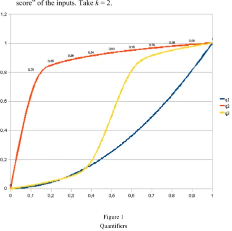
(i) Let a quantifier q1 : [0,1] → [0,1] by given by q1(x) = xp, p > 1. Then OWA operator AW’∆q1 prefers the “high score” of the inputs. Take p = 2.
(ii) Let a quantifier q2: [0,1] → [0,1] by given by q2(x) = xp, p א ]0,1[. Then
OWA operator AW’∆q2 prefers the “low score” of the inputs. Take p = 0,1.
(iii) Let a quantifier q3: [0,1] → [0,1] by given by q3(x) = [1 + (2x-1)p]/2, p =
1/(2k+1) and k א N. Then OWA operator AW’∆q3 prefers the “average
score” of the inputs. Take k = 2.
Figure 1 Quantifiers
Conclusion
We have introduced some other decision making methods to show another view of the ranking of the public universities and their faculties. We have used all three procedures of linear input data normalization and applied five chosen aggregation operators and three multicriteria methods to it, in order to compare them with the ARRA ranking. ARRA creates its ranking based on the normalization Procedure 1 and on the simple arithmetic mean (average) as an aggregation method. It is one of the possible choices for composing them.
As we have seen in the previous examples, the results (rankings) by using the same aggregation methods for different normalization procedures are not the same. We have shown that they depend firstly on the choice of the normalization
procedure and secondly on aggregation method. The chosen aggregation operators show us that Procedure 3 of linear input data normalization seems to be the best way, because by using different aggregation methods, rankings are very similar.
Recall that all of these methods and many others are only a support for a decision maker.
Acknowledgement
This work was supported by APVV-0012-07 and VEGA 1/0080/10 grants.
Table 8
Summary of the rankings based on chosen aggregation operators and multicriteria methods
References
[1] Calvo T., Kolesárová A., Komorníková M., Mesiar R. (2002): Aggregation Operators: Properties, Classes and Construction Methods, in: Studies in Fuzziness and Soft Computing-Aggregation Operators. New Trends and Applications (T. Calvo, G. Mayor, R. Mesiar editors), Physica-Verlag, Heidelberg, pp. 3-106
[2] Calvo T., Mayor G., Torrens J., Suner J., Mas M., Carbonell M. (2000):
Generation of Weighting Triangles Associated with Aggregation Functions, Int. J. Uncertainty, Fuzziness and Knowledge-Based Systems, 8, pp. 417- 451
[3] Calvo T., Mayor G., Mesiar R. (2002): Aggregation Operators: New Trends and Applications, Studies in Fuzziness and Soft Computing, Physica- Verlag Heidelberg New York, Vol. 97, pp. 44-47
[4] Grabisch M., Marichal J.-L., Mesiar R., Pap E. (2009): Aggregation Functions, Cambridge University Press, Cambridge
[5] Pomerol Ch., Barba-Romero S. (2000): Multicriterion Decision in Management: Principles and Practice, Kluwer Academic Publishers, Boston
[6] Yager R. R. (1988): On Ordered Weighted Averaging Aggregation Operators in Multicriteria Decision Making, IEEE Transactions on Systems, Man and Cybernetics 18, pp. 183-190
[7] Taylor A. D. (1995): Mathematics and Politics: Strategy, Voting, Power and Proof, Springer-Verlag, pp. 96-127
[8] www.arra.sk
[9] Michel Grabisch, Jean-Luc Marichal, Radko Mesiar, Endre Pap:
Monograph: Aggregation Functions, in Acta Polytechnica Hungarica, Vol.
6, No. 1, 2009, pp. 79-94