Multi-Source Coded Downloads

Multi-Source Coded Downloads

Patrik J. Braun^∗†, Derya Malak^∗, Muriel Médard^∗

∗Research Laboratory of Electronics (RLE) Massachusetts Institute of Technology

Cambridge, MA 02139 USA {pbraun, deryam, medard}@mit.edu

Péter Ekler^†

†Department of Automation and Applied Informatics Budapest University of Technology and Economics

Budapest, 1111 Hungary {patrik.braun, peter.ekler}@aut.bme.hu

Abstract—In this paper, we propose a selective-repeat (SR) automatic repeat-request (ARQ) model for multi-source down- load scenarios and analyze their useful throughput that we refer to as goodput. The multi-source scenario comprises a set of transmitters that send packets to a receiver. We characterize the forward channels from the transmitters to the receiver via a general hidden Markov model (HMM) and assume that the reverse channels from the receiver to the transmitter are lossless.

To find the average goodput of the network, we exploit the probability-generation function. We consider different packet transmission schemes, including uncoded random, network coded and sliding window-based network coded packets, and contrast their performance. Our calculations show that using network coding in a multi-source scenario can increase the average goodput, while sliding window-based coding may also archive the theoretical maximum goodput. We show that our multi-source approach avoids the straggler problem, therefore adding more transmitters to the network increases its throughout and the system does not get limited by the weakest transmitter. We also verify our analytic results with extensive simulations.

Index Terms—Network coding, selective-repeat (SR), Auto- matic Repeat-reQuest (ARQ), Hidden Markov model (HMM), Multi-source network, Throughput.

I. INTRODUCTION

Automatic Repeat reQuest (ARQ) is a widely used er- ror control method for data transmissions. It uses timeouts and acknowledgments (ACKs) to achieve reliable transmis- sion over an unreliable channel and has several well known types including Stop-and-wait ARQ, Go-Back-N ARQ, and selective-repeat (SR) ARQ. In case of SR ARQ, the transmitter sends packets without waiting for their ACK and only the lost packets are selectively retransmitted. ARQ has been applied in modern networks to boost their throughput and reliability [1],[2] and there are detailed analytical models to calculate its throughput: it has been shown that if the average packet-error rate is, the throughput of SR ARQ with reliable feedback is 1 − [3]. Y. J. Cho and C. K. UN analyzed different ARQ models with forward and backward channels memory [4] and showed that error bursts have a significant impact on throughput. In [5], Ausavapattanakun and Nosratinia suggested a more versatile, hidden Markov model (HMM) based approach for analyzing SR ARQ with a discrete channel model.

We have recently extended the work of Ausavapattanakun and showed that using erasure coding, e.g.: random linear net- work coding (RLNC) on ARQ channels models may increase

the throughput by up to 40% [6]. M. Tömösközi et al. showed their coded sliding window approach outperforms the Reed- Solomon and other RLNC approaches in per-packet delay [7].

J. K. Sundararajan et al. introduced a network coded (NC) approach to transmission control protocol (TCP) and showed that their scheme achieves a much higher throughput compared to TCP over a lossy link [8].

Most of the ARQ approaches work on a point-to-point basis that can be used in single-receiver single-transmitter networks, but they do not support multi-source scenarios. Multi-source download has a huge potential in future 5G networks, where users are using mobile networks to access bandwidth and delay intensive services, like video streaming. It has been shown through measurements that multi-source video streaming may help to meet this bandwidth and delay constraints, since it increases download throughput and reliability, and thereby the quality of service [9]. Furthermore, using network coded shared file system for multi-source download with four com- mercial cloud solutions may achieve up to five-fold increase in download speed compared to single-source download [10].

M. Sipos showed a six-fold increase in download speed by using four commercial clouds and a custom network coded protocol [11]. While these works show huge potential of multi- source download, they mainly do it through measurement results and lack a rigorous analytical model.

In this paper, we propose an SR ARQ model to analyze the multi-source networks, inspired by the point-to-point model in [5] and [6]. The analysis focuses on goodput, the useful throughput of the network. Our model containsN transmitters (with N orthogonal channels) and one receiver. Our forward link is modeled by a hidden Markov model (HMM). We con- sider not only the conventional uncoded transmission schemes but also the rateless coded and sliding window-based coding methods. We show that the sliding window-based coding may reach optimal goodput. The uncoded scheme also converges to the optimal goodput with the increase of the window size on the transmitter. Our results also show that applying rateless codes on the transmitted data may further increase goodput.

Furthermore, the straggler problem is a huge challenge in distributed systems [12]. Results also show that our approach avoids the straggler problem, thus increasing the number of transmitters, increases goodput without getting limited by the weakest transmitter. We also compare our analysis with simulation results. To the best of our knowledge, this paper

is the first to consider an HMM-based channel model, which also incorporates RLNC in a multi-source network scenario.

II. SYSTEM MODEL

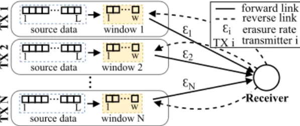
We focus on multi-source networks, where there are N transmitters and only one receiver. Each transmitter has its own channel, but all transmitters have the same source data, i.e. the set of original packets: L={p₁, . . . ,p_L}, whereL is the total number of packets. The receiver aims to collect the setL. We consider that the receiver has an infinite receive-side window. While each transmitter has access to all L packets, it also maintains aw-sized window, where w<L. An overview about the proposed multi-source system is shown in Fig. 1.

...

L 1

source data window 1

Receiver

1 w

...

...

reverse link forward link

Ɛ Ɛ Ɛ

Ɛ erasure rate 1

2

N i

...

L 1

source data window 2

1 w

...

...

L 1

source data window N

1 w

...

TX 1TX 2TX N

TX i transmitter i

Fig. 1. Multi-source system overview.

A. Channel model

Each transmitter has an unreliable forward link (the channel from the transmitter to the receiver) and a lossless reverse link (the channel from the receiver to the transmitter) that does not interfere with other links. All links are delayed: we assume the round trip time (RTT) is fixed and is equal for each transmitter and given by κ_c = κ_ct→r+κ_cr→t, where κ_ct→r is the latency between the transmitter and the receiver, while κ_cr→t is the latency between the receiver and the transmitter.

We model the erasures on the forward link with a hidden Markov model to make our solution applicable to different types of channels, similarly to the work of Ausavapattanakun and Nosratinia [5]. At every time slot, a transmitter sends a packet that may be delivered or lost due to an erasure.

The outcome of a transmission through channel i, denoted by X_t⁽ⁱ⁾, is a Bernoulli random variable, taking values from X⁽ⁱ⁾={0,1}, where 0 and1 correspond to an erroneous and an error-free transmission, respectively. The channel condition is model by a multistate Markov chainS_t⁽ⁱ⁾, in which the states are S⁽ⁱ⁾={1, . . . ,K⁽ⁱ⁾}, and its probability transition matrix is P_(i). Each stateS⁽_tⁱ⁾=j,j∈S⁽ⁱ⁾has a different error probability _j⁽ⁱ⁾. We denote the set of these channel error probabilities by ⁽ⁱ⁾ = {⁽ⁱ⁾

1 , . . . , ⁽ⁱ⁾

K⁽ⁱ⁾}. The process X_t⁽ⁱ⁾, which is driven by the Markov process S_t⁽ⁱ⁾ is a hidden Markov process and can be characterized by {S⁽ⁱ⁾,X⁽ⁱ⁾,P_(i), ⁽ⁱ⁾}. Furthermore P_L,(i) = P(i)·diag{⁽ⁱ⁾} and P_R,(i) = P(i)·diag{1−⁽ⁱ⁾} are the probabilities of losing and receiving a packet, respectively.

Note that P_L,(i)+P_R,(i)=P(i).

Furthermore, our model does not use an explicit channel coding, but it can be applied on the top of a network that uses channel coding. We assume that the underlying layers use some channel coding that can indicate if a packet was lost.

B. Protocol Description

In our model, the source of a packet is not important as long as the receiver receives that packet. Thus to avoid the race condition in a parallel multi-source system and make the analysis simpler, we assume for our analysis that the transmitters are scheduled in a round-robin fashion. In every time slot, only one transmitter sends a packet. The RTT for this round-robin model will be: k=Nκ_c and also k_r→t =Nκ_cr→t and k_t→r=Nκ_ct→r. As a result of round-robin scheduling of the transmitters in ascending order, a packet received at time slott is sent by transmitter:

s(t)=

(N if(tmodN)=0

(t modN)otherwise, (1)

and transmitters(t) sends:

pkt(t)=packet arrives or gets lost at the receiver at timet. (2) The life cycle of a packet is the following:

1) packet scheduling and sending: In every time slot, a transmitter selects a packet from their w-sized window and sends it over their channel.

2) packet arrives or gets lost: Receiver sends a feedback κ_ct→r time slots after the transmitter sent the packet, independent of whether the packet got lost or arrived at the receiver.

3) receiving the feedback:κ_cr→tlater the feedback arrives at the transmitter, which updates its window content based on the feedback.

Since a transmitter sends a packet in every time slot and the reverse link is perfect, transmitters receive an ACK or NACK in every slot as well. A transmitter selects a packet to send based on a pre-determined scheduling method that is the same for every transmitter. We detail the different scheduling methods in Section IV.

We do not consider conventional SR ARQ protocol in our analysis since not all lost packets need to be retransmitted automatically: We use cumulative feedback that contains all previously received packets at the receiver (from all trans- mitters). If a subset of the channels wants to transmit packet p_l ∈ L and it gets lost on some of the channels, but received through at least one of the channels, all transmitters will receive an ACK corresponding to packetp_l. Therefore, it is not necessary and also redundant to retransmit packet p_l on any of the channels. Fig. 2 gives an example of our round-robin transmission model.

12

1 2 1 2 1 2

transmitter #

time slot 1 2 3 4 2

1 1 2 1 2

5 6 7 8 9 10 11 time slots

transmitter 1 sends packet p

receiver sends feedback to packet p

receiving the feedback k = 8

k_{r→t = 4} k_{t→r = 4}

Fig. 2. Timeline example for serialized model withN=2,k=8.

In our analysis, we assume that the transmitters cannot com- municate with each other, which makes the packet scheduling

challenging. We measure the receiver status with its Degrees of Freedom (DoF). DoF at the receiver increases if it receives a new, useful packet that contains new information. Due to the lack of cooperation, several transmitters may schedule the same packet for transmission, and the receiver may receive duplicate packets that do not increase its DoF.

Data download in our system has a push fashion instead of a centralized, receiver-driven pull fashion, because of the cumulative feedback and the lack of cooperation. Due to this push fashion, a transmitter can schedule any not yet acknowledged packet without depending on other transmitters.

Therefore the system is not limited by the weakest transmitter and avoids the straggler problem.

We focus on estimating the goodput of a multi-source system in our analysis. We define goodput as the number of DoF increases at the receiver per sent packet. We distinguish goodput η(i)∈ [0,1] for channeli and goodputη ∈ [0,N] for the whole system.

III. ANALYSIS

In this section we describe a method for analyzing the overall and per channel average goodput of a system with N transmitters. First, we detail the possible outcomes of packet transmission.

In the forward channel, during transmission, a packet can get:

1) E_L,(i) (lost): the event that a packet is lost with P_L,(i)

probability on channeli,

2) E_R,(i)(received): the event that a packet is received with P_R,(i) probability on channeli.

During scheduling time, a transmitter might schedule a packet that is:

1) E_pU,(i) (potentially useful): the event that given E_R,(i), the packet will increase the DoF at the receiver, 2) E_pD,(i)(potentially duplicate): the event that givenE_R,(i),

the packet will not increase the DoF at the receiver.

If the packet is received, it might be

3) E_U,(i) (useful): the event that a packet is successfully received on channel i and increases the DoF at the receiver,

4) E_D,(i)(duplicate): the event that a packet is successfully received on channeli, but does not increase the DoF at the receiver.

Event E_L,(i) and E_D,(i) are equivalent, since in both cases receiver does not receive new DoFs in that time slot. Therefore, these two events can be combined into a single event:

5) E_F,(i) (fail): packet was lost, or it was received on channeli, but does not increase the DoF at the receiver.

Using these events, we define the following two main probabilities:

P_U,(i)=P(E_U,(i))

P_F,(i)=P(E_F,(i)) (3) Based on (3), we construct a signal-flow graph [13] to model the goodput of individual channels. We use matrix branch

gains in the graph, since each link has multiple states because we use HMM to model them. A signal-flow graph is a diagram of directed branches between nodes to visually represent a system of equations. Nodes are variables of the equations, while the branches are the relationships between the variables.

Basic equivalences, like parallel, series, self-loop can be used to simplify a flow graph [14]. A signal-flow graph with matrix branch transmissions and vector node values is a matrix signal- flow graph (MSFG).

We construct the MSFG in such a way that branch gains appear as pz^x, where xis the random variable of interest and p is a probability. Thereby the graph represents an equation system that is polynomial in z with coefficients that are the probabilities of a given value of x. This system of equations is theE[zⁿ], the probability generation function (PGF) forx.

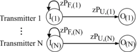
Fig. 3 shows the matrix flow graph of our transmission model. In the figure, state I_(i) represents the transmission of a new packet, while at state O_(i), the feedback of eventE_U,(i) is received at the transmitteri and the transmitter can update its window accordingly.

Transmitter 1

...

Transmitter N

zP_F,(1)

zP_F,(N) I(1)

I_(N)

zP_U,(1)

zP_U,(N) O(1)

O_(N)

Fig. 3. Matrix signal-flow graph for goodput analysis of our serialized model.

Next, we calculate the transmission time τ that we define as the number of transmitted packets per DoF increase at the receiver. τ can be calculated by using the matrix-generating function Φ_τ(z). We get Φ_τ,(i)(z) by applying basic node reduction on the MSFG, similarly to [5]:

Φ_τ,(i)(z)=(I−zP_F,(i))⁻¹zP_U,(i), (4) whereIis the identity matrix.

To calculate the PGF, we need to express π_I(i), the proba- bility vector of eventE_U,(i). In this case, it isπ_I(i)=π(i)P_U,(i), whereπ(i)is the stationary vector ofP(i)and can be found by solving:

π_(i)P_(i)=π_(i)

π(i)1=1, (5)

where1is the column vector of ones. Furthermore, let_F,(i)be the packet-failure rate: _F,(i)=π_(i)P_F,(i)1. Then PGF of φ_τ(z) can be calculated by pre- and post-multiplying Φ_τ(z)with a row and a column vector, respectively:

φ_τ(i)(z)= π_I(i)Φ_τ,(i)(z)1

π_I(i)1 = 1 1−_F,(i)

π_(i)P_U,(i)Φ_τ,(i)(z)1.

(6) The average transmission time of transmitter i, τ_(i) can be obtained by evaluating the first derivative of PGF φ_τ(i)(z) at z =1. The goodput, η_(i) of channel i is the reciprocal is the average transmission time, i.e., η(i)=1/τ(i).

A. Calculating the probability of sending a useful packetP_U,(i) and a packet failure P_F,(i)

Whether a packet pt received at timet is potentially useful depends only on the lastktime slots: Packet pt is sent at time ts = t −kt→r, since the transmitter-receiver latency is kt→r. Transmitters(t_s)has a feedback that contains information from time t_s−k_r→t = t−k, since the receiver-transmitter latency is k_r→t (i). Furthermore, transmitters can also keep records of previously sent packets (ii) . Since the transmitters may not cooperate, a transmitter may only use information (i) and (ii) to schedule a packet for transmission.

Using the feedback from time t−k, it is guaranteed that a transmitter will not send a packet that would be a duplicate of packets before timet−k, but it has no information about the packets after that time. Therefore it may schedule duplicates with them. We assume that a transmitter does not schedule packets that are duplicates with its previously sent packets¹. Thus, a packet at time t will not be useful only if it has the same information as any of the useful packets in the last k time slots. There may be u ∈ [0,k−^N_k]useful packets² sent by transmitters j, j,s(t) between time slotst−k andt.

We next investigate the number of potentially duplicates sent by transmitters(t). If the packet from transmitters(t)is a potentially duplicate of a useful packet from any transmitter j, j,s(t), then the probability is higher that the packet at time t is useful (since if a duplicate packet was already transmitted by transmitters(t)in the lastktime, it will not retransmit that packet. Thus it is more likely to choose a useful packet).

1 2 1 2 1 2

transmitter # time slot

2

1 1 2 1 time slots

k = 8

event pD F pU U pU F pD U ?

F: fail

U: useful pU: potentially useful pD: potentially duplicate -

-

1 2 3 4 5 6 7 8 9 10 11

k_{r→t = 4} k_{t→r = 4}

Fig. 4. Example realization to calculateP_U,(i)and P_F,(i),N=2,k=8.

To better understand our methodology, let us consider the following example for N =2, k =8, as shown in Fig. 4. In this example, we are interested in calculating the probability that the packet received at time t =11 from transmitter 1 is useful. We know that the receiver obtainedu=2packets from transmitter 2 in the last k=8 time slots. The packet at time t =11 may be a duplicate of any of those 2 useful packets.

The Packet at time t =9 from transmitter 1 is a potentially duplicate with any of the packets from transmitter 2 between time slots [2,8]. If it is a duplicate of the packet at timet=6, our investigated packet at timet=11may only be a duplicate (if it is a duplicate at all) with packet at time 10.

Rest of this section uses this methodology to express P_U(i) and P_F,(i) as a function of t through several steps. At every step, we express the probability of a packet being useful or to fail (is duplicate or lost) based on a given condition and

1Throughout our analysis we do not use forward error correction, therefore packet pwill be only rescheduled for transmission if a NACK for packetp is received.

2Sincek=Nκc, thus(Nmodk)=0

also the probability of that given condition. To obtain P_U(i) andP_F,(i), we define the following quantities at timet:

v∈ {0,1}^t,v_l=

(1 if E_R,(s(l))

0 otherwise, (7)

wherevrepresents a possible channel outcome between time slots [0,t].

ByE_r(v), we denote the event thatvis the channel outcome between[0,t]time slots. We define the probability ofvas the channel outcome, P_r(v) = P(E_r(v)). The packet at time t is being useful or fail, conditioned on v:

P_cU(v)=P(E_U,(s(t)) at timet | E_r(v))

P_cF(v)=P(E_F,(s(t)) at timet |E_r(v)) (8) Note that all probabilities with v as parameter, now im- plicitly depends on the transmitter, since v = [v₁. . .v_t] is the input of the function and only transmitter i = s(t) may transmit at timet. Therefore, we can also omit the transmitter from P_U(i)(t)andP_F,(i)(t)and express them as follows:

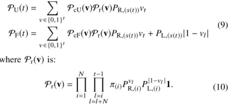
P_U(t)= Õ

v∈ {0,1}^t

P_cU(v)P_r(v)P_R,(s(t))v_t

P_F(t)= Õ

v∈ {0,1}^t

P_cF(v)P_r(v)P_R,(s(t))v_t+P_L,(s(t))|1−v_l| (9)

whereP_r(v)is:

P_r(v)= ÖN

i=1

Öt−1

l=l+Nl=i

π(i)P_R,(i)^vl P_L,(i)^|1−vl|1. (10)

The probabilities P_cU(v)and P_cF(v) depend on the proba- bility of a packet being potentially useful or duplicate:

P_pU(v)=P(E_pU,(s(t)) at timet | E_r(v))

P_pD(v)=P(E_pD,(s(t)) at timet | E_r(v)) (11) and they may be expressed the following way:

P_cU(v)=P_pU(v)^vt+0^|1−vt|

P_cF(v)=P_pD(v)^vt+1^|1−vt|. (12) As (12) shows, a packet is useful with probability P_pU(v)if it is received and fails with probability P_pD(v) if received or with probability 1if lost.

To calculate P_pU(v) and P_pD(v), the following quantities need to be expressed:

a∈ {0,1}^k,aj =













’x’ ifs(t−j)=s(t) 1 else ifE_U,(s(t−j))

0 otherwise

b∈ {0,1}^k,b_i =























’x’ ifs(t−i),s(t) 1 else ifEpD,(s(t−i)), and

∃j,0<i≤k,E_U,(s(t−j)), pkt(t−i) ≡pkt(t−j) 0 otherwise,

(13)

where x means the value at that position will not be used during our calculations, but to simplify our formulas, we assume its value to be 0. pkt(i) ≡ pkt(j) means that two packets are interchangeable, i.e., they increase the DoF at the receiver by at most one. Vectorarepresents the useful packets received from transmitterj,j ,s(t)between time slots[t−k,t], b represents the potentially duplicates with any useful packet between [t−k,t] and received from transmitters(t)between time slots [t−k,t].

We define the probability that there is a useful packet with a givena=[a_i, . . . ,a_k]for every potentially duplicate packet inb=[b_i, . . . ,b_k]:

E_dp(a,b)=∀i,b_i =1 :∃j,j <i,a_j =1 pkt(t−i) ≡pkt(t−j) P_dp(a,b)=P(E_dp(a,b)).

(14)

We also define P_outcome(v,a,b) as the probability ofa and b is the outcome between time slots[t−k,t]:

P_outcome(v,a,b)=P(∀a_j =1,E_U,(s(t−j)),

∀a_j =0,E_D,(s(t−j)),

∀b_i =1,EpD,(s(t−i)) |E_dp(a,b),E_r(v)) (15)

Furthermore, we define P_sU(a,b)andP_sD(a,b), the probabili- ties of a packet at timetbeing useful or duplicate, respectively, conditioned ona andb:

P_sU(a,b)=P(E_U,(t) |E_dp(a,b))

P_sD(a,b)=P(E_D,(t) |E_dp(a,b)) (16) Using eqs. (13) to (16), we can express P_pU(v):

P_pU(v)=

k−_N^k

Õ

u=0 k N

Õ

d=0

Õ

Íaj=u Íbi=d

P_dp(a,b)P_sU(a,b)P_outcome(v,a,b) (17) whereuis the number of useful packets sent by the transmitter j, j , s(t). d is the number of packets that are sent by the transmitter s(t)and are potentially duplicate packets with the useful packets in the last k time slots. Similarly to P_pU(v), we can also express P_pD(v) by using P_sD(a,b), instead of P_sU(a,b).

P_dp(a,b) and P_outcome(v,a,b) can be expressed in the fol- lowing way:

P_dp(a,b)=

k

Ö

s(t−l)l=1=s(t)

Íl

j=1a_j−Íl i=1b_i k− _N^k

P_outcome(v,a,b)=

k

Ö

j=1 s(t−j),s(t)

P_cU(v_t−j)^ajP_cF(v_t−j)|^1−aj| ·

Ök

i=1 s(t−i)=s(t)

P_pD(v_t−i)^bi(P_pU(v_t−i)+P_pD(v_t−i))^|1−bi|

v_t−l =[v₁. . .v_t−l].

(18)

The presented equations in this section do not depend on the method how a transmitter selects a packet for transmission, but to calculate P_sU(a,b) andP_sD(a,b), one also has to consider the applied packet scheduling method. We detail that in the next section. Furthermore, our matrix-flow graph approach to calculate the average goodput is only applicable if lim

t→∞P_U(t) and lim

t→∞P_F(t) exist.

IV. SCHEDULING METHODS

In this section, we enumerate several packet scheduling strategies. We calculate P_sU(a,b) and P_sD(a,b), that are re- quired to calculate the average goodput in (17), corresponding to a given scheduling method.

As described in Section II, transmitters maintain aw-sized window. We consider a moving window instead of a sliding window that we define the following way: If a packet gets removed from the window, the next available packet will be picked from the L source data to fill the window. Therefore, the window constantly contains w packets³. We assume L is large enough, so that there are always enough packets to fill the window, which is the case in a streaming scenario.

A. Sufficient genie scheme

We introduce a sufficient geniescheduling strategy to find the optimal goodput of a system with the given channel properties. It is not a full genie, since it only focuses on sending the perfect packet regarding usefulness, but packets might be lost on the channel. Therefore, P_sU(a,b) = 1 and P_sD(a,b)=0.

Using a genie, the transmitter-channel pairs can be de- coupled and analyzed independently. The average goodput of transmitter i only depends on the loss probability P_L,(i). Following the steps in [5], the average goodput of a channel i is:

η_(i)=1−_(i)=1−π_(i)P_L,(i)1. (19) The overall average goodput of the system for N transmit- ters isη=ÍN

i=1η_(i).

B. Uncoded random scheme

In this approach, transmitters select a not-in-flight⁴ packet uniformly at random from their send window for transmission.

We can expressP_sU(a,b)andP_sD(a,b)in the following way:

P_sU(a,b)=1− P_sD(a,b)=w−_N^k − (Ík

j=1a_j−Ík i=1b_i) w−_w^k

(20) where _N^k is the number of packets in flight from one transmit- ter, and the summation gives how many useful packets were sent by transmitter j, j ,s(t) in the last k time slot in such a way that the transmitter s(t) has not sent any potentially duplicate packet to those packets.

3The packet in our window may not be consecutively chosen and there is no limit on the maximum time a packet can spend in the window.

4A packet is in flight when it is sent, but feedback has not been received.

C. Rateless RLNC coded schemes

RLNC creates linear combinations of original packets with randomly chosen coefficients. It may be applied to the trans- mitted data to reduce the probability of receiving duplicate packets. RLNC has recoding ability and can work as a rateless code over a fixed set of packets [11] or as a sliding window code over a changing set of packets [15].

In this scheme, we use RLNC in a rateless coding way:

packets are grouped into generations, creating altogetherG∈ Z⁺generations withg∈Z⁺ packets in each. Network coding is applied to each of thegenerations. Each transmitter groups the packets in the same way, but uses a different random seed to generate the linear combinations. In our analysis, we assume that the field size used is high enough such that the probability of two encoded packets being linearly dependent goes to zero [16]. The receiver feedback contains the rank of a generation instead of information about an individual packet, where the rank equals the DoF of a given generation.

The transmitter window contains Gw = ^w_g generations⁵. In every time slot, a transmitter chooses one generationfrom its window to create an encoded packet from and sends it over the channel. The selection of a generation may be based on different approaches. In this paper, we investigate a random and a rarest first generation selection schemes.

In both cases, P_sU(a,b) and P_sD(a,b) depend on the probability of transmitter s(t) choosing the generation γ for transmission and its rank at time slott. Calculating these prob- abilities is not part of this paper. We instead show the goodput of applying network coding in a multi-source environment through simulations in Section V.

1) Random generation selection scheme: Transmitters choose a generation for transmission uniformly at random.

2) Rarest first generation selection scheme: Transmitters approximate the rank of the generations an the receiver and choose the one that hase the least rank. The approximation is based on two components: 1) the feedback that represents the receiver state k_r→t time slots ago, 2) the sent packets by that given transmitter. We call this strategy rarest generation first strategy, referring to the rarest piece first algorithm in BitTorrent [17].

One should note two special cases that apply for both generation selection approaches: 1) if g = 1, the goodput will be identical with the uncoded random schemes. 2) if L =w = g, the goodput will be identical with the sufficient genie scheme, since all received packet will be useful.

D. Coded sliding window scheme

In case of the network coding sliding window [15] scheme, a transmitter encodes all the packets in its window with RLNC. The receiver feedback contains information about the successfully decoded packets. The probability of receiving a useful packet is the following:

5To keep the analysis simple, we assumeLmodg=wmodg=0.

P_sU(a,b)=1− P_sD(a,b)=

(1 if (tmodk)<w

0 otherwise . (21)

Note that if k ≤ w, all received packets will be useful, therefore the strategy would have the same goodput as the sufficient geniescheme.

Comparing this solution to the rateless RLNC coded strate- gies, sliding window achieves optimal performance with cod- ing less or equal packets together, thereby using less CPU cycles, since we usually have k << L. On the other hand, with rateless coding the random seed can be shared between the transmitter and the receiver, while with sliding window the coefficient vector needs to travel in the packet payload.

V. NUMERICAL RESULTS

We computed the numerical results for our model by using a two state Gilbert-Elliot (GE) channel model [18] for the forward link of the transmitters. The state-transition matrix of the channel is given by:

P(i)=

1−q_(i) q_(i) r_(i) 1−r_(i)

, (22)

where the first row corresponds to the good (G) state and the second to the bad (B) state. The channel error probability is ⁽ⁱ⁾ = {_G⁽ⁱ⁾, _B⁽ⁱ⁾} = {0,1}. The packet loss rate _F,(i) can be calculated from⁽ⁱ⁾and the stationary vector ofP(i) as shown in Section III.

We use our simulator testbed to analyze the goodput of our data scheduling schemes. Each simulation was run 1000 times, and an average is calculated from them. We compare our simulations and numerical results and they show similar trends.

ε1 ε1 ε1 ε2 ε1

ε2 ε1 ε2 ε3

ε1 ε2 ε3

ε1 ε2 ε3 ε4

ε1 ε2 ε3 ε4

ε1 ε2 ε3 ε4 FRQQHFWLRQW\SHSDFNHWORVVUDWHFKDQQHO

JRRGSXWη

VXIIJHQLHDQDO\WLFDO VXIIJHQLHVLPXODWLRQ XQFRGHGUQGDQDO\WLFDO XQFRGHGUQGVLPXODWLRQ

UQGJHQ5/1&g = 3VLPXODWLRQ UDUHVWILUVWJHQ5/1&g = 12VLPXODWLRQ VOLGLQJZLQGRZ5/1&DQDO\WLFDO VOLGLQJZLQGRZ5/1&VLPXODWLRQ

Fig. 5. Goodput for transmittersN=[1,2,3,4], RTTκc=3, window size w=24and burst rater=0.3.

Fig. 7 shows that apart from the sufficient genie and the coded sliding windowscheme, that have the achievable maxi- mum goodput, window size has a high impact on goodput:

small window size causes a significant goodput decrease, since the transmitters have a smaller set of packets to choose from. As the figure also shows, in caserarest first generation selection scheme, goodput also depends on the combination of the window size and the generation size.

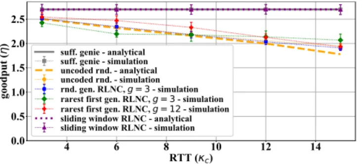
Higher RTT values have a negative impact on goodput, as Fig. 6 shows. Rarest first generation selection scheme may perform better compared to theuncoded random, but the gain depends on both generation size and RTT. With low RTT, the bigger generation size, while with high RTT the smaller generation size performs better.

Increasing the number of transmitters increases overall average goodput, but increases the chance of sending duplicate packets for theuncoded randomscheme or the rateless RLNC coded schemes, as Fig. 5 shows, since the difference between the achievable maximum and the actual throughput increases.

577κc

JRRGSXWη VXIIJHQLHDQDO\WLFDO VXIIJHQLHVLPXODWLRQ XQFRGHGUQGDQDO\WLFDO XQFRGHGUQGVLPXODWLRQ UQGJHQ5/1&g = 3VLPXODWLRQ UDUHVWILUVWJHQ5/1&g = 3VLPXODWLRQ UDUHVWILUVWJHQ5/1&g = 12VLPXODWLRQ VOLGLQJZLQGRZ5/1&DQDO\WLFDO VOLGLQJZLQGRZ5/1&VLPXODWLRQ

Fig. 6. Goodput for transmittersN=3, packet loss rate_F,(i)=0.1, window sizew=24and burst rater=0.3.

ZLQGRZVL]Hw

JRRGSXWη VXIIJHQLHDQDO\WLFDO

VXIIJHQLHVLPXODWLRQ XQFRGHGUQGDQDO\WLFDO XQFRGHGUQGVLPXODWLRQ UQGJHQ5/1&g = 3VLPXODWLRQ UDUHVWILUVWJHQ5/1&g = 3VLPXODWLRQ UDUHVWILUVWJHQ5/1&g =^w₃VLPXODWLRQ VOLGLQJZLQGRZ5/1&DQDO\WLFDO VOLGLQJZLQGRZ5/1&VLPXODWLRQ

Fig. 7. Goodput for transmitters N = 3, RTT κc = 4, packet loss rate F,(i)=0.1and burst rater=0.3.

VI. CONCLUSION

In this paper, we proposed an SR ARQ model for multi- source single-receiver download. The model uses lossy for- ward links that are modeled with a hidden Markov process.

We used a matrix signal-flow graph approach to calculate the probability generation function of the goodput, and to analyze the average goodput of a multi-source download system.

We compared numerical results with simulation results for several packet scheduling approaches, including the uncoded and network coded approaches. Our results show that rateless network coding techniques can boost goodput, while network coded sliding window may achieve optimal performance.

We also showed that our multi-source approach avoids the straggler problem, therefore adding new transmitters to the network increases the goodput.

In this paper, we analyzed a moving window approach does not set any constraints on the packet delay. As future work, we

plan to investigate a more flexible window approach that has a constraint on the delay and we would like to also consider further packet scheduling schemes.

ACKNOWLEDGMENTS

This research was supported by the BME-Artificial Intel- ligence FIKP grant of EMMI (BME FIKP-MI/SC), by the János Bolyai Research Fellowship of the Hungarian Academy of Sciences and by the Fulbright and Rosztoczy programs.

REFERENCES

[1] 3GPP, “Study on new radio access technology Phys- ical layer aspects,” 3rd Generation Partnership Project (3GPP), Technical report (TR) 38.802, 09 2017. [On- line]. Available: https://portal.3gpp.org/desktopmodules/Specifications/

SpecificationDetails.aspx?specificationId=3066

[2] S. R. Khosravirad and H. Viswanathan, “Analysis of Feedback Error in Automatic Repeat reQuest,”CoRR, vol. abs/1710.00649, 2017.

[3] D.-L. Lu and J.-F. Chang, “Performance of ARQ protocols in noninde- pendent channel errors,”IEEE Transactions on Comm., vol. 41, no. 5, pp. 721–730, May 1993.

[4] Y. J. Cho and C. K. Un, “Performance analysis of ARQ error controls under Markovian block error pattern,” IEEE Transactions on Comm., vol. 42, no. 234, pp. 2051–2061, FEBRUARY 1994.

[5] K. Ausavapattanakun and A. Nosratinia, “Analysis of Selective-Repeat ARQ via Matrix Signal-Flow Graphs,”IEEE Transactions on Comm., vol. 55, no. 1, pp. 198–204, Jan 2007.

[6] M. M. D. Malak and E. M. Yeh, “Analysis of Coded Selective-Repeat ARQ via Matrix Signal-Flow Graphs,” CoRR, vol. abs/1801.10500, 2018.

[7] M. Tömösközi, F. H. P. Fitzek, D. E. Lucani, M. V. Pedersen, and P. Seeling, “On the Delay Characteristics for Point-to-Point Links using Random Linear Network Coding with On-the-Fly Coding Capabilities,”

in20th European Wireless Conf., May 2014, pp. 1–6.

[8] J. K. Sundararajan, D. Shah, M. Médard, S. Jakubczak, M. Mitzen- macher, and J. Barros, “Network Coding Meets TCP: Theory and Implementation,”Proceedings of the IEEE, vol. 99, no. 3, pp. 490–512, March 2011.

[9] J. Bruneau-Queyreix, M. Lacaud, D. Negru, J. M. Batalla, and E. Bor- coci, “MS-Stream: A multiple-source adaptive streaming solution en- hancing consumer’s perceived quality,” in14th IEEE CCNC, Jan 2017, pp. 427–434.

[10] C. W. Sørensen, D. E. Lucani, and M. Médard, “On network coded filesystem shim: Over-the-top multipath multi-source made easy,” in IEEE ICC, May 2017, pp. 1–7.

[11] M. Sipos, F. H. P. Fitzek, D. E. Lucani, and M. V. Pedersen, “Distributed cloud storage using network coding,” inIEEE 11th CCNC, Jan 2014, pp. 127–132.

[12] M. A. M. Songze Li and A. S. Avestimehr, “A Unified Coding Framework for Distributed Computing with StragglingServers,”CoRR, vol. abs/1609.01690, 2016.

[13] S. J. Mason and H. J. Zimmermann, “Electronic circuits, signals, and systems,” pp. xviii, 616 p., companion volume to Electronic circuit theory, by H.J. Zimmermann and S.J. Mason.

[14] R. A. Howard,Dynamic probabilistic systems: Markov models. Courier Corporation, 2012, vol. 1.

[15] S. Wunderlich, F. Gabriel, S. Pandi, and F. H. P. Fitzek, “We don’t need no generation - a practical approach to sliding window RLNC,” in2017 Wireless Days, March 2017, pp. 218–223.

[16] T. Ho, M. Médard, R. Koetter, D. R. Karger, M. Effros, J. Shi, and B. Leong, “A Random Linear Network Coding Approach to Multicast,”

IEEE Transactions on Inf. Theory, vol. 52, no. 10, pp. 4413–4430, Oct 2006.

[17] A. Legout, G. Urvoy-Keller, and P. Michiardi, “Rarest First and Choke Algorithms Are Enough,” in 6th ACM SIGCOMM Conf. on Internet Measurement, ser. IMC ’06. New York, NY, USA: ACM, 2006, pp.

203–216.

[18] E. O. Elliott, “Estimates of error rates for codes on burst-noise channels,”

The Bell System Tech. Journal, vol. 42, no. 5, pp. 1977–1997, Sept 1963.