PatrikJ.Braun,DeryaMalak,MurielMédard,PéterEkler GoodputAnalysisforMulti-SourceCodedDownloads

Goodput Analysis for Multi-Source Coded Downloads

Patrik J. Braun, Derya Malak, Muriel Médard, Péter Ekler

Abstract

Multi-source download comprise a set of sources that send packets to a receiver. In this paper, we focus on a scenario, where sources cannot communicate with each other, which makes the packet scheduling challenging: sources may send the same packet to the receiver, which results in a throughput drop. Applying coding, such as Random Linear Network Coding (RLNC) on the transmitted packets may help to overcome this issue. Instead of collecting individual packets, the receiver collects RLNC encoded packets that have a higher chance to increase the Degree of Freedom (DoF) at the receiver’s end, as they are the combination of multiple packets.

In this paper, we propose a selective-repeat (SR) Automatic Repeat-reQuest (ARQ) model for multi-source download. We introduce an analytical framework to analyze six multi-source protocols, including uncoded, rateless RLNC, and sliding-window based RLNC protocols and contrast their goodput (application-level throughput). Our analysis shows that employing RLNC in a multi-source network improves goodput, in particular sliding window-based RLNC protocol achieves the maximum theoretical goodput. In addition, we show that our multi-source approach avoids the straggler problem, therefore adding more sources to the network increases its goodput. We also verify our analytical results with extensive simulations.

Index Terms

Automatic Repeat-reQuest (ARQ), Goodput, Hidden Markov model (HMM), Selective-Repeat (SR), Network Coding, Multi-source network.

Patrik J. Braun, Derya Malak and Muriel Médard are with the Network Coding and Reliable Communications Group, RLE, MIT, Cambridge, Massachusetts, 02139 USA, e-mail: {pbraun, deryam, medard}@mit.edu.

Patrik J. Braun, Péter Ekler are with the Department of Automation and Applied Informatics, VIK, Budapest University of Technology and Economics, Budapest, 1117 Hungary, e-mail: {braun.patrik, ekler.peter}@aut.bme.hu.

This work has been done, when Patrik J. Braun was a visiting student researcher at MIT.

This research was supported by the BME-Artificial Intelligence FIKP grant of EMMI (BME FIKP-MI/SC), by the János Bolyai Research Fellowship of the Hungarian Academy of Sciences and by the Fulbright and Rosztoczy programs.

I. INTRODUCTION

Multi-source download involves a single receiver requesting the same data from multiple data sources. It has high potential in information-centric networking (ICN) [1], especially in an Internet of Things (IoT) or a Vehicle-to-Vehicle (V2V) communication environment [2]. In both IoT and V2V setup, the network contains a set of data sources that potentially have the same data, and a receiver aims to obtain that data. An example of this scenario is as follows: Consider a group of cars traveling on the highway and sharing all of their sensor information with each other. When a new car joins the group and wants to download that sensor information as well, the most efficient way of doing so is to request this data from multiple sources.

There have been several works on multi-source data transfer: Hashmeni and Bohlooli mod- eled multi-source content delivery through multi-path transmission in ICNs [1]. They estimated virtual round-trip time (VRTT) between the receiver and a group of sources in their proposed model. They selected this VRTT as a key parameter of performance evaluation that can be used to calculate the network throughput. A congestion control mechanism for Content-Centric Networking (CCN) with multi-source content retrieval was proposed by Miyoshi et al. [3]. Their solution uses end-to-end flow control to regulate the transmission only on the congested paths.

Thomas et al. designed a multi-source and multipath File Transfer Protocol (mmFTP) for ICN networks [4]. They showed through measurements that mmFTP has 37% throughput increase compared to a single-source download, while it avoids congested paths or sources. In a video streaming environment, multi-source download also improves network bandwidth and delay, and thereby the quality of service [5]. Our solution differs from previous works by providing an analytical framework for estimating the goodput (i.e., the useful throughput of the network) of different multi-source protocols.

In a multi-source scenario, managing the packet scheduling at the different sources is a challenging task, especial in a loosely orchestrated scenario, like in V2V communication, where the set of available sources are continuously changing. In these environments, multiple sources may schedule the same data packet that does not contain new information to the receiver. To avoid this issue, coding can be applied to the source packets.

An early version of coded data transfer was rateless codes like fountain codes that often did not use feedback [6]. However, to have flow control in a transmission, feedback is required. Malak et al. analyzed Selective-Repeat (SR) Automatic Repeat reQuest (ARQ) channel models that use

erasure coding (like Random Linear Network Coding (RLNC)) with feedback [7]. They showed that RLNC increases the throughput by up to 40% in SR ARQ channels. Liu et al. presented a solution for network coded multi-source transmissions in ICN [8]. They collaborated in-network caching with network coding to increase transmission efficiency. We also proposed a system for downloading YouTube videos from multiple sources that support uncoded, and RLNC encoded multi-source protocols [9]. Our measurement results showed that our uncoded protocol could outperform a simple parallel HTTP approach, while applying coding, it is possible to reach up to a three-fold goodput increase. It has also been shown that using a network coded shared file system for multi-source download with four commercial cloud solutions may achieve up to five- fold increase in download speed compared to single-source download [10]. Furthermore, Sipos showed a six-fold increase in download speed by using four commercial clouds and a custom network coded protocol [11]. In this work, we propose RLNC based multi-source protocols and contrast their performance with uncoded multi-source protocols by using our analytical framework.

Apart from achieving flow control, feedback can also be used to improve the performance of coding. Sundararajan et al. used feedback to acknowledge degrees of freedom (DoF) (the number of useful packets arrived at the receiver) instead of original decoded packets [12]. Using this feedback, they proposed a network coding method that can be performed in an online manner, without the need for grouping packets into batches of generations. They also introduced a network coded approach to transmission control protocol (TCP) and showed that their scheme achieves a ten fold throughput increase compared to TCP on a link with 1% loss rate [13]. They presented a sliding window network coding approach, where they used the feedback to adjust the window of packets that they coded on. Kim et al. presented a model to analyze the performance of TCP with network coding [14]. They showed that network coding could prevent TCP’s performance degradation that is often observed in lossy networks. Tömösközi et al. showed that RLNC coded sliding window approach outperforms the Reed-Solomon, and other rateless RLNC approaches in terms of per-packet delay [15]. In this paper, we use the RLNC coded sliding window approach in a multi-source download scenario and contrast its goodput with uncoded and rateless RLNC encoded multi-source protocols by using our analytical framework.

In a distributed system, the straggler problem is also a challenge [16] [17]. If the client has to wait for a packet that is unusually late to arrive, the network throughput may drop. In this paper, we propose a solution that avoids the straggler problem.

In this paper, we extend our previous work on coded multi-source download [18]. We build on singe-source singe-receiver SR ARQ model of Ausavapattanakun and Nosratinia [19], and the RLNC encoded SR ARQ model of Malak et al. [7] and extend them to support multi-source downloads. We propose an analytical framework to investigate the performance of six multi- source protocols, including uncoded and RLNC encoded protocols. The main contributions of this paper can be summarized as follows:

• Section II proposes an SR ARQ model to analyze a general multi-source network, inspired by the point-to-point model in [7] and [19]. Our model contains N data sources (with N orthogonal forward and backward links) and one receiver. We use a hidden Markov model (HMM) to model the transmission states on the forward links. We assume that feedback is perfect

• Section III presents an analytical framework to analyze our multi-source network model and calculate its goodput. We construct our analysis in a way that it is independent of the used packet scheduling strategy.

• Section IV enumerates six packet scheduling strategies for multi-source protocols, including approaches where sources send uncoded, rateless RLNC and sliding window based RLNC encoded packet. Furthermore, we also consider a sufficient genie scheduling strategy that has the theoretical maximum goodput in a multi-source network. In Section IV, we also propose two moving windowapproaches on the sender side that better fit for a multi-source scenario than the conventional sliding window solution: onemoving windowwithout packet delay constraint and the other one is with the constraint. We also apply our goodput analysis from Section III to these scheduling strategies with both moving window approaches and calculate their goodput.

• Section V presents our analytical results. We also verify our analysis with extensive simu- lations.

• Section VI summarizes our work and suggests further research.

The significance of our work is that we show that RLNC encoded sliding window-based approach may reach the optimal goodput. The uncoded protocol also converges to the optimal goodput with the increase of the window size on the sources. Our results also show that applying rateless RLNC encoding on the transmitted data may further increase goodput. Furthermore, results also show that our approach avoids the straggler problem, thus increasing the number of

sources, increases goodput without getting limited by the weakest sources. To the best of our knowledge, this paper is the first to consider an analytical model for multi-source networks that also incorporates RLNC.

II. SYSTEM MODEL

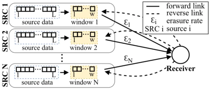
We focus on multi-source networks, where there are N sources and only one receiver. Each source has its own link (channel), but all sources have the same original data, i.e., the set of original packets: L = {p₁, . . . ,p_L}, where L is the total number of packets. The receiver aims to collect the set L. We consider that the receiver has an infinite receive-side window. While each source has access to all L packets, it also maintains a w-sized window, where w ≤ L. An overview of the proposed multi-source system is shown in Fig. 1.

...

L 1

source data window 1

Receiver

1 w

...

...

reverse link forward link

Ɛ Ɛ Ɛ

Ɛ erasure rate 1

2

N i

...

L 1

source data window 2

1 w

...

...

L 1

source data window N

1 w

...

SRC 1SRC 2SRC N

SRC i source i

Fig. 1. Multi-source system overview.

A. Link model

Each data source has an unreliable forward link (the channel from the source to the receiver) and a lossless reverse link (the channel from the receiver to the source) that does not interfere with other links. All links are delayed: we assume the round trip time (RTT) is fixed and is equal for each sources and given by κc = κ_cs→r+κ_cr→s, where κ_cs→r is the number of time slots to transmit a packet from the source to the receiver, while κ_cr→s is the number of time slots to send an ACK from the receiver to the source.

We model the transmission status with a hidden Markov model that is driven by a multi-state Markov process to make our solution applicable to different types of links, similarly to the work of Ausavapattanakun and Nosratinia [19]. At every time slot, a source sends a packet that may be delivered or lost due to erasure. The outcome of a transmission through link i, denoted by

X_t⁽ⁱ⁾, is a Bernoulli random variable, taking values fromX⁽ⁱ⁾ ={0,1}, where0 and 1correspond to an error-free and an erroneous transmission, respectively. The link condition is modeled by a multistate Markov chain S_t⁽ⁱ⁾, in which the states are S⁽ⁱ⁾ = {1, . . . ,K⁽ⁱ⁾}, and its probability transition matrix is P_(i). Each state S_t⁽ⁱ⁾ = j,j ∈ S⁽ⁱ⁾ has a different error probability ⁽ⁱ⁾_j . We denote the set of these link error probabilities by ⁽ⁱ⁾ ={₁⁽ⁱ⁾, . . . , ⁽ⁱ⁾

K⁽ⁱ⁾}. The process X_t⁽ⁱ⁾, which is driven by the Markov process S_t⁽ⁱ⁾ is a hidden Markov process and can be characterized by {S⁽ⁱ⁾,X⁽ⁱ⁾,P(i), ⁽ⁱ⁾}. Furthermore P_L,(i) = P(i) ·diag{⁽ⁱ⁾} and P_R,(i) = P(i) ·diag{1−⁽ⁱ⁾} are the probabilities of losing and receiving a packet, respectively. Note that P_L,(i)+P_R,(i) = P_(i).

In or model we consider an abstract link layer, provided on the network that can detect packet losses. The link and the the underlying network layers may or may not use additional channel coding, but we do not take that into consideration in our calculations.

B. Protocol Description

In a multi-source scenario, sources send a packet in every time slot. In out model, the receiver sends feedback to all sources, and the reverse link is perfect. Therefore, sources receive an ACK or NACK in every slot. The life cycle of a packet is the following:

1) packet scheduling and sending: In every time slot, a source selects a packet from their w-sized window and sends it over their link.

2) packet arrives or gets lost: Receiver sends feedback to all sources κ_cs→r time slots after the source sent the packet, independent of whether the packet gets lost or arrives at the receiver.

3) receiving the feedback: κ_cr→s time slots later, the feedback arrives at the source, which updates its window content based on the feedback.

A source selects a packet to send based on a pre-determined scheduling method that is the same for every source. We detail the different scheduling methods in Section IV.

We do not consider conventional SR ARQ protocol in our analysis since not all lost packets need to be retransmitted automatically: We use cumulative feedback that contains all previously received packets at the receiver (from all sources). If a subset of the sources wants to transmit packet p_l ∈ L and it gets lost on some of the links but received through at least one of the links, all sources will receive an ACK corresponding to packet p_l. Therefore, it is redundant to retransmit packet p_l on any of the links.

In our analysis, we assume that the sources cannot communicate with each other, which makes the packet scheduling challenging. We measure the receiver status with its Degrees of Freedom (DoF). DoF at the receiver increases if it receives a new, useful packet that contains new information. Due to the lack of cooperation, several sources may schedule the same packet for transmission, and the receiver may receive duplicate packets that do not increase its DoF.

Data download in our system has a push fashion instead of a centralized, receiver-driven pull fashion since the sources decide which packet to send and not the receiver requests them. Fur- thermore, due to the cumulative feedback and the lack of cooperation, a source can schedule any not yet acknowledged packet without depending on other sources. Since the packet scheduling at a source is independent of the other sources, introducing a new source to the system will not limit the other sources. Thus the system avoids the straggler problem.

We focus on estimating the goodput of a multi-source system in our analysis. We define goodput as the increment in the number of DoF at the receiver per sent packet. We distinguish goodput η(i) ∈ [0,1] of link i and goodput η ∈ [0,N] for the whole system.

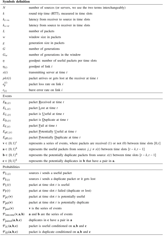
The notation of this paper is summarized in TABLE I.

III. GENERALANALYSISAPPROACH

In this section, we describe a general framework for analyzing the overall and per link goodput of a system with N sources. We construct this framework such a way that it is independent of the applied multi-source protocol. Then, in Section IV we enumerate several multi-source protocols and use this framework to compute their goodput.

A. Round-robin source scheduling

Due to the multi-source scenario, the receiver may receive up-to N packets in each time slot (at most one from each source, but some might get lost). If two or more packets are the same (i.e., they increase the DoF at the receiver only by one), at most one of them may be useful, and the rest is duplicate. A packet is duplicate or useful depending on the order that the receiver processes them. In our model, the source of a packet is not important as long as the receiver successfully receives that packet. Thus to avoid the race condition in a parallel multi- source system and make the analysis simpler, we assume for our analysis that the sources are scheduled in a round-robin fashion. Hence, in every time slot, only one source sends a packet. A further benefit of this round-robin approach is that we can analyze each packet separately when

TABLE I SYMBOLS LIST

Symbols definition

N number of sources (or servers, we use the two terms interchangeably) k round trip time (RTT), measured in time slots

k_r→s latency from receiver to source in time slots ks→r latency from source to receiver in time slots

L number of packets

w window size in packets

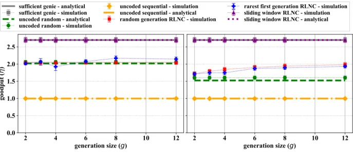
g generation size in packets

G number of generations

G_w number of generations in the window

η goodput: number of useful packets per time slots η_(i) goodput of linki

s(t) transmitting server at timet

pkt(t) packet arrives or gets lost at the receiver at timet _F⁽ⁱ⁾ packet loss rate on linki

r_(i) burst error rate on linki Events

E_R,(t) packet Received at timet E_L,(t) packet Lost at timet E_U,(t) packet is Useful at timet E_D,(t) packet is Duplicate at timet E_F,(t) packet Fail at timet

E_pU,(t) packet Potentially Useful at timet E_pD,(t) packet Potentially Duplicate at timet

v∈ {0,1}^t represents a series of events, where packets are received (1) or not (0) between time slots[0,t] a∈ {0,1}^k represents the useful packets from source j,j,s(t)between time slots[t−k,t−1]

b∈ {0,1}^k represents the potentially duplicate packets from source s(t) between time slots[t−k,t−1]

c∈ {0,1}^k represents the potentially duplicates inb that have a pair ina.

Probabilities

P_U,(i) sourcesisends a useful packet

P_F,(i) sourcesisends a duplicate packet or it gets lost P_U(t) packet at time slottis useful

P_F(t) packet at time slottfailed (duplicate or lost) P_pU(v) packet at time slottis potentially useful P_pD(v) packet at time slottis potentially duplicate P_past(v) vis the series of events

P_outcome(v,a,b) aandbare the series of events P_paired(a,b,c) duplicates inchave a pair in a

P_sU(a,b,c) packet is useful conditioned ona,bandc P_sD(a,b,c) packet is duplicate conditioned ona,b andc

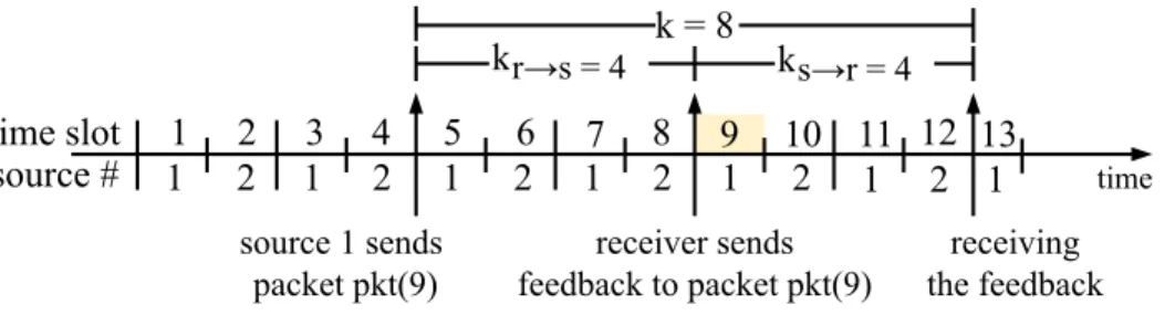
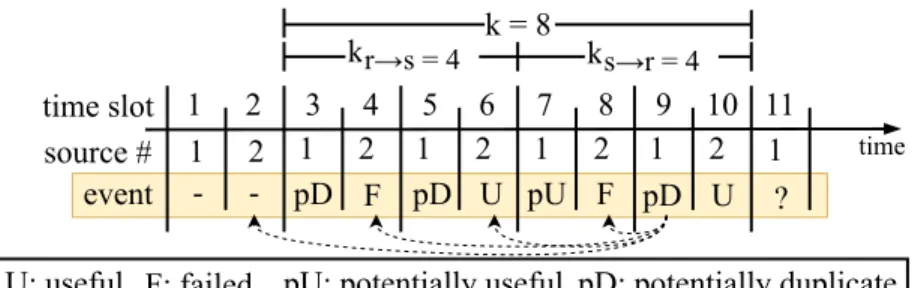
calculating the goodput. Thus a goodput increase in our model is not the result of having higher bandwidth (through more sources) but result of sending packets in a more efficient way. The RTT for this round-robin model will be: k = Nκ_c and also k_r→s = Nκ_cr→s and k_s→r = Nκ_cs→r. Fig. 2 gives an example of our round-robin transmission model.

12

1 2 1 2 1 2

source #

time slot 1 2 3 4 2

1 1 2 1 2

5 6 7 8 9 10 11

time source 1 sends

packet pkt(9)

receiver sends feedback to packet pkt(9)

receiving the feedback k = 8

k_{r→s = 4} k_{s→r = 4} 13

1

Fig. 2. Timeline example for serialized model withN=2sources and, RTTk=8.

As a result of round-robin scheduling of the sources in ascending order, a packet received at time slot t is sent by source:

s(t)=













N if (t mod N)= 0 (t modN) otherwise,

(1)

and source s(t) sends:

pkt(t)=packet arrives or gets lost at the receiver at time t. (2)

B. Taxonomy of transmission events

To calculate the goodput of a multi-source system, we detail the possible outcomes of packet transmission first. In the forward link, during transmission, a packet can get:

1) E_L,(i) (lost): the event that a packet is lost with P_L,(i) probability on link i,

2) E_R,(i) (received): the event that a packet is received with P_R,(i) probability on link i.

During scheduling time, a source might schedule a packet that is:

1) E_pU,(i) (potentially useful): the event that given E_R,(i), the packet will increase the DoF at the receiver,

2) E_pD,(i) (potentially duplicate): the event that given E_R,(i), the packet will not increase the DoF at the receiver.

If the packet is received, it might be

3) E_U,(i) (useful): the event that a packet is received on link i and increases the DoF at the receiver,

4) E_D,(i) (duplicate): the event that a packet is received on link i, but does not increase the DoF at the receiver.

Event E_L,(i) and E_D,(i) are equivalent, since in both cases receiver does not receive new DoFs in that time slot. Therefore, these two events can be combined into a single event:

5) E_F,(i) (failed): packet was lost, or it was received on link i, but does not increase the DoF at the receiver.

C. Technical approach

Using these events, we define the probability of a packet is useful or the transmission failed:

P_U,(i) = P(E_U,(i)) P_F,(i) = P(E_F,(i))

(3) Based on (3), we construct a signal-flow graph [20] to model the goodput of individual links.

We use matrix branch gains in the graph since each link has multiple states because we use HMM to model them. A signal-flow graph is a diagram of directed branches between nodes that visually represent a system of equations. Nodes are variables of the equations, while the branches are the relationships between the variables. Basic equivalences, like parallel, series, self-loop can be used to simplify a flow graph [21]. A signal-flow graph with matrix branch transmissions and vector node values is a matrix signal-flow graph (MSFG).

We construct the MSFG in such a way that branch gains appear as pz^X, where X is the random variable of interest and p is a probability. Thereby the graph represents an equation system that is polynomial in z with coefficients that are the probabilities of a given value of X. This system of equations is E[zⁿ], the probability generation function (PGF) for X.

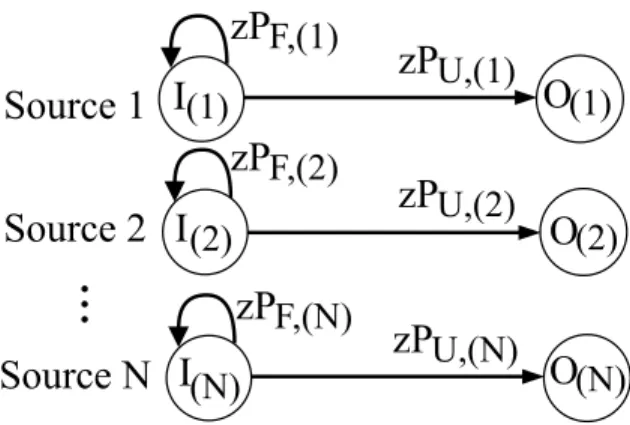
Fig. 3 shows the matrix flow graph of our transmission model. In the figure, state I(i)represents the transmission of a new packet, while at state O(i), the feedback of event E_U,(i) is received at the source i and the source can update its window accordingly.

Next, we calculate the transmission time τ that we define as the number of sent packets per DoF increase at the receiver.τcan be calculated by using the matrix-generating functionΦ_τ,(i)(z).

We get Φ_τ,(i)(z) by applying basic node reduction on the MSFG, similarly to [19]:

Φ_τ,(i)(z)= (I−zP_F,(i))⁻¹zP_U,(i), (4)

Source 1

...

Source 2

Source N

zP

zP

zP

I

I

I

zP

zP

zP

O

O

O

Fig. 3. Matrix signal-flow graph for goodput analysis of our serialized model.

where I is the identity matrix.

To calculate the PGF, we need to express πI(i), the probability vector of event E_U,(i). In this case, it is πI(i) =π(i)P_U,(i), where π(i) is the stationary vector of P(i) and can be found by solving:

π(i)P_(i) =π(i)

π(i)1=1, (5)

where 1 is the column vector of ones. Furthermore, let _F⁽ⁱ⁾ be the packet-failure rate: _F⁽ⁱ⁾ = π(i)P_F,(i)1. Then PGF of φτ(z) can be calculated by pre- and post-multiplying Φ_τ(z) with a row and a column vector of πI(i) and 1, respectively:

φ_τ(i)(z)= πI(i)Φ_τ,(i)(z)1

π_I(i)1 = 1

1−_F⁽ⁱ⁾π(i)P_U,(i)Φ_τ,(i)(z)1. (6) The average transmission time of sourcei,τ(i) can be obtained by evaluating the first derivative of PGF φτ(i)(z)at z= 1. The goodput, η(i) of link i is the reciprocal is the average transmission time, i.e., η(i) =1/τ(i)1.

D. Calculating the probability of sending a useful packet P_U,(i) and a packet failure P_F,(i) Whether a packet pkt(t) is received at time t is potentially useful depends only on the last k time slots: Packet pkt(t) is sent at time t_s = t − k_s→r, since the source-receiver latency is k_s→r. (i) The Source, that sends pkt(t), has a feedback that contains information from time t_s − k_r→s = t− k, since the receiver-source latency is k_r→s. (ii) Furthermore, sources can also

1This is indeed a lower bound due to the Jensen’s inequality [22] and the convexity of1/τ_(i).

keep records of previously sent packets. Since the sources may not cooperate, a source may only use information (i) and (ii) to schedule a packet for transmission.

Using the feedback from time slot t−k, it is guaranteed that a source will not send a packet that would be a duplicate of packets before time slot t − k, but it has no information about the packets after that time (i.e., packets sent between [t−k,t−1]). Therefore it may schedule duplicates with them. We assume that a source does not schedule packets that are duplicates with its previously sent packets². Thus, a packet at time t will be duplicate only if it has the same information as any of the useful packets in the last k time slots. There may be u ∈ [0,k− _N^k] useful packets³ sent by sources j, j , s(t) between time slots [t−k,t−1].

We next investigate the number of potentially duplicates sent by source s(t) between time slots [t−k,t−1]. If a packet from source s(t) is a potentially duplicate of a useful packet from any source j, j , s(t), then the probability is higher that the packet at timet is useful (since if a duplicate packet was already transmitted by source s(t) in the last k time, it will not retransmit that packet. Thus it is more likely to choose a useful packet).

1 2 1 2

source # time slot

2

1 1 2 1 ^time

event pD F pD U pU F pD U ?

1 2 3 4 5 6 7 8 9 10 11

- -

1 2

k = 8

k_{r s = 4} k_{s r = 4}

F: failed

U: useful pU: potentially useful pD: potentially duplicate

Fig. 4. Example realization to calculate P_U,(i)andP_F,(i), N=2sources and RTTk=8.

To better understand our methodology, let us consider the following example for N = 2, k = 8, as shown in Fig. 4. In this example, we are interested in calculating the probability that the packet received at time t = 11 from source 1 is useful. We know that the receiver obtained u = 2 packets from source 2 in the last k = 8 time slots. The packet at time t = 11 may be a duplicate of any of those two useful packets. The packet at time t = 9 from source 1 is a potentially duplicate with any of the packets from source 2 between time slots [2,8]. If it is a

2Throughout our analysis, we do not use forward error correction. Therefore a source reschedules a packet only if it has received a NACK for that packet.

3Sincek=Nκc, κc∈Z⁺, thus(kmodN)=0

duplicate of the packet at time t = 6, our investigated packet at timet = 11 may be a duplicate (if it is a duplicate at all) with the packet at time slot 10.

Rest of this section uses this methodology to expressP_U(i) andP_F,(i) as a function oft through several steps. At every step, we express the probability of a packet to be useful or failed. To obtain P_U(i) and P_F,(i), we define vector v = [v₁. . .vt], the series of event, where packet are received or lost between time slots [1,t]. We express v as follows:

v ∈ {0,1}^t, vl =













1 if E_R,(s(l)) 0 otherwise.

(7)

Usingv, we can define the probabilities that a packet is potentially useful or duplicate at time:

P_pU(v)=P(EpU,(s(t)) at time t | v ) P_pD(v)=P(EpD,(s(t)) at time t | v )

(8)

Furthermore, we defineP_past(v₁. . .vt−1)as the probability of[v₁. . .vt−1]is the series of events between time slots [1,t−1]:

P_past(v₁. . .v_t−1)=P(v₁. . .v_t−1)

=

N

Ö

i=1

t−1

Ö

l=i (l−imodN)=0

π(i)P^v_R,(i)^l P_L,(i)^|1−vl|1, (9)

where π(i) is the stationary vector of P(i) and 1 is a column vector of ones, as defined above.

Note that all probabilities that are conditioned on v, now implicitly depend on the source, since v is the input of the function and only source s(t) may transmit at time t. Therefore, we will omit the source index from P_U(i)(t) and P_F,(i)(t) and express them as follows:

P_U(t)= Õ

v∈{0,1}^t

P_pU(v)P_past(v₁. . .vt−1)P_R,(s(t))vt

P_F(t)= Õ

v∈{0,1}^t

P_pD(v)P_past(v₁. . .v_t−1)P_R,(s(t))vt +(1−vt)P_L,(s(t)), (10) where we consider all possible series of packet lose or receive events and calculate P_U(t) as the probability of a packet is potentially useful and it was received. We get P_F(t) by calculating the probability of a packet potentially duplicate, and it was received, or it was lost.

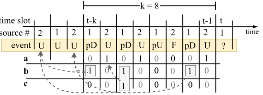
As shown previously in Fig. 4, to calculate if a packet is potentially useful or duplicate at time t, we need to consider the events in the last k time slots, therefore we define the following quantities:

1

1 2 2 1 2

source # time slot

2

1 1 2 1 ^time

k = 8

event

t U F pD pU U pD pD U

F: failed

U: useful pU: potentially useful pD: potentially duplicate t-k

a b c

0 1 0 1 0 0 0 1

1 0 1 0 0 0 1 0

0 0 1 0 0 0 0 0

2

U

U U

t-1

?

Fig. 5. Example configuration of vectorsa,bandcwithN=2sources and RTTk=8.

1) a∈ {0,1}^k (useful vector): indicates if a packet from any source j,j , s(t) was useful or failed in the last k time slots.

2) b∈ {0,1}^k (duplicates vector): indicates if source s(t) sent a potentially duplicate packet in the last k time slots. Note that b does not specify if the duplicate packet is duplicate with a useful packet from time slots[k−t,t−1] or before that time.

3) c∈ {0,1}^k (matched duplicates vector): indicates if source s(t)sent a potentially duplicate packet in the last k time slots and that potentially duplicate packet is a duplicate with a useful packet from time slots [k−t,t−1] (i.e., for every 1 in c, there is a unique pair in a). Note thatc_i is1 if and only if b_i =1. Fig. 5 shows a possible configuration of vectors a,b, c.

4) P_paired(a,b,c) represents the probability that a,b,c are valid, i.e.: all potentially duplicate packets in b have a useful packet pair, while duplicates inc has a useful packet pair in a.

5) P_outcome(v,a,b) represents probability that events a and b occur, conditioned on v.

6) P_sU(a,b,c) and P_sD(a,b,c) represent the probabilities of a packet is useful or duplicate, respectively, conditioned on events a,b and c.

We define these quantities formally as follows:

a∈ {0,1}^k, a_j =



















’undefined’ if s(t− j)= s(t) 1 else if E_U,(s(t−j))

0 otherwise

b∈ {0,1}^k, b_i =



















’undefined’ if s(t−i), s(t) 1 else if EpD,(s(t−i))

0 otherwise

c ∈ {0,1}^k, c_i =

































’undefined’ if s(t−i), s(t) 1 else if EpD,(s(t−i)), and

∃j,0 ≤ j < i, E_U,(s(t−j)), pkt(t−i) ≡ pkt(t− j)

0 otherwise,

(11)

where ’undefined’ means that the source at that time slot is not active, but to simplify our for- mulas, we assume its value to be0. pkt(i) ≡ pkt(j)means that two packets are interchangeable, i.e., receiving both packets would only increase the DoF at the receiver by at most one.

We formally define E_paired(a,b,c), the event that there is a useful packet with a given a = [a₁, . . . ,a_k] for every potentially duplicate packet in b=[b₁, . . . ,b_k], as follows:

E_paired(a,b,c)=∀i,c_i = 1 :∃j,j < i,a_j = 1

pkt(t−i) ≡ pkt(t− j). (12)

Using E_paired(a,b,c), we define its probability, P_paired(a,b,c) as follows:

P_paired(a,b,c)=P(E_paired(a,b,c)). (13)

We also define P_outcome(v,a,b), the probability of events a and b occur between time slots [t−k,t−1], conditioned on v:

P_outcome(v,a,b)=P(∀aj =1, E_U,(s(t−j)),

∀a_j =0, E_D,(s(t−j)),

∀b_i =1, EpD,(s(t−i)) | E_paired(a,b,c),v )

(14)

Furthermore, we define P_sU(a,b,c) and P_sD(a,b,c), the probabilities of a packet at time t being useful or duplicate, respectively, conditioned on a, b and c:

P_sU(a,b,c)= P(E_U,(t) | E_paired(a,b,c) ) P_sD(a,b,c)= P(E_D,(t) | E_paired(a,b,c) )

(15)

Using eqs. (11) and (13) to (15), we can express the probabilities of a packet at time t is potentially useful or duplicate, respectively:

P_pU(v)=

k−_N^k

Õ

u=0

k

ÕN

d=0 min(d,u)

Õ

m=0

Õ

Ía_j=u Íb_i=d Íc_i=m,c_i≤b_i

P_paired(a,b,c) P_sU(a,b,c)P_outcome(v,a,b)

P_pD(v)=

k−_N^k

Õ

u=0

k

ÕN

d=0 min(d,u)

Õ

m=0

Õ

Ía_j=u Íb_i=d Íc_i=m,c_i≤b_i

P_paired(a,b,c) P_sD(a,b,c)P_outcome(v,a,b).

(16)

P_paired(a,b,c) in (16) can be expressed in the following way:

P_paired(a,b,c)=

k

Ö

l=1 s(t−l)=s(t)

b_l=1

c_l − Íl

j=1a_j−Íl−N i=1 c_i k− _N^k

. (17)

We get everyl, where b_l = 1and we calculate the probability that every duplicate (ci =1) has a pair in a, (aj =1, j < i), such that a_j = 1 was not paired previously. Furthermore if c_i = 0, but b_i = 1, we consider the probability of packet pkt(t− (k−i)) is duplicate with a useful packet between time slots [1,t−k −1].

P_outcome(v,a,b) in (16) can be expressed in the following way:

P_outcome(v,a,b)=

k

Ö

j=1 s(t−j),s(t)

(P_pU(vt−j)vt−j)^aj(P_pD(vt−j)vt−j +(1−vt−j))|^1−aj|

k

Ö

i=1 s(t−i)=s(t)

P_pD(vt−i)^biP_pU(vt−i)^|1−bi|

vt−l =[v₁. . .vt−l],

(18)

Where the first row of the equation calculates the probability of source j,j , s(t) sent a useful packet or the transmission failed. The second row calculates the probability of source s(t) sent a potentially useful or duplicate packet.

To calculateP_sU(a,b,c)andP_sD(a,b,c), one also has to consider the applied packet scheduling strategy. We detail that in the next section.

Furthermore, our matrix-flow graph approach to calculate the goodput is only applicable if

t→∞lim P_U(t) and lim

t→∞P_F(t) exist.

IV. MULTI-SOURCE PROTOCOLS

In this section, we enumerate several packet scheduling strategies for the multi-source proto- cols. We calculateP_sU(a,b,c)andP_sD(a,b,c), that are required to calculate the potential duplicate and useful probabilities in (16), corresponding to a given scheduling method.

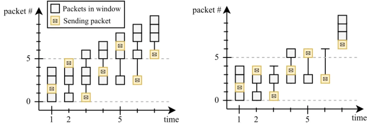
As described in Section II, sources maintain a w-sized window. Most of the SR ARQ models use a sliding window approach to send packets. Packets with the lowest packet id are chosen from the window for transmission. If a packet with the lowest id gets successfully transmitted, it can be removed from the window, and the window can slide to include new packets. In a multi-source scenario, we cannot use this conventional sliding window, since in that case, all servers would send the same packet. Therefore, in this paper, we consider a moving window setup. In a moving window setup, any packet can be chosen for scheduling (i.e., the transmitted packets do not have to be in consecutive order). We differentiate between strict moving window and sparse moving window. Fig. 6 shows an example of the two moving windowapproaches.

5 packet #

time

1 2 5

0

packet #

time Packets in window

Sending packet

1 2 5

5

0

Fig. 6. Example of sparse moving window (left) and strict moving window (right).

a) Sparse moving window: If a packet gets removed from the window, the next available packet will be picked from theL source data to fill the window. Therefore, the window constantly

contains w packets⁴. We assume L is large enough so that there are always enough packets to fill the window, which is the case in a streaming scenario. Note that this window does not have any constraint on the packet delay.

b) Strict moving window: To introduce a constraint on packet delay to sparse moving window, we define W(t), the set of packets in a strict moving window at time t the following way:

W(t)= {i ∈ L | w_min ≤ i ≤ w_min+w−1}

L = {0, . . . ,L}

L_acked(t)= {i ∈ L | packet i was acknowledged by time t}

w_min = min(L\L_acked(t)),

(19)

where L is the set of the original data packets, L_acked(t) is the set of all successfully received and acknowledged packets by timet andw_min is a not-yet-acknowledged packet with the lowest index.

Using our window models, we consider the following scheduling approaches: 1) sufficient genie that gives the optimal scheduling with the given link conditions, 2) uncoded sequential, which is a simple approach for packet scheduling, 3) uncoded random, that aim is to exploit the multi-source network in a more efficient way than the uncoded sequential, 4)RLNC rateless coded that applies network coding to a group of source packets and those coded packets travel the network, 5) RLNC sliding window that uses network coding in a sliding window fashion to create coded packets.

A. Sufficient genie

We introduce a sufficient genie scheduling strategy to find the optimal goodput of a system with the given link properties. It is not a full genie since it only focuses on sending the perfect packet (i.e., the most useful packet), but packets might get lost on the link. The goodput is the same for both moving window approaches:

P_sU(a,b,c)=1 P_sD(a,b,c)=0.

(20)

4The packet in our window may not be consecutively chosen and there is no limit on the maximum time a packet can spend in the window.

Using a genie, the source-link pairs can be decoupled and analyzed independently. The goodput of source i only depends on the loss probability P_L,(i). Following the steps in [19], the goodput of a link i is:

η(i) = 1−_F⁽ⁱ⁾ =1−π(i)P_L,(i)1. (21)

The overall goodput of the system for N sources is η= ÍN i=1η(i). B. Uncoded sequential

In the case of uncoded sequential, a source sends packets in a sequential fashion. If a packet gets lost on all the links, each source reschedules that packet. This scheduling strategy uses the window in a first in, first out (FIFO) fashion. The first packet of the window gets scheduled, while if a packet is lost it is added to the end of the window. Since we assume that the sources are scheduled in a round-robin fashion, every source transmits the same packet between time slots [x,x+ N], x ∈ Z⁺,(x mod N) = 0. Therefore, only one of the packets may be useful in that interval. A packet is useful with probability 1 if no useful packet was received in the last s(t) −1 time slots:

P_sU(a,b,c)=1− P_sD(a,b,c)=

(1−min(

k

Õ

j=k−s(t)−1

a_j,1))

, (22)

where |x| is the absolute value of x. This also means that if s(t)= 1 the probability is always 1. Therefore the maximum goodput of the uncoded sequential approach is η=ÍN

i=1η(i) ≤ 1.

Uncoded sequential behaves similarly with both window approaches. In the case of strict moving window, the window may get empty. In our model we assume that the window never gets empty. Therefore, (22) will not hold for strict moving window. The window can only get empty if the same packet gets lost repeatedly from all the sources, while all the other packets are transmitted. This has a low probability. Thus we can use (22) to estimate the goodput of theuncoded sequential approach with astrict moving window. We use simulations to verify this estimation in Section V.

C. Uncoded random

In this approach, sources select a not-in-flight⁵ packet uniformly at random from their send window for transmission. The probabilities P_sU(a,b,c) and P_sD(a,b,c) depend on the window model:

a) Sparse moving window: The probabilities can be expressed the following way:

P_sU(a,b,c)=1− P_sD(a,b,c)= w− (_N^k − (d−m)) − (u−m) w− (_N^k − (d−m)) u=Õk

j=1a_j d =Õk

i=1b_i m=Õk

i=1c_i

(23)

where _N^k is the number of in-flight packets from source s(t). u is the number of useful packets sent by source j, j , s(t). d ≤ _N^k is the number of duplicates sent by source s(t), and m < d is the number of duplicates sent by source s(t) and these packets are duplicates with packets in the last k time slot. _N^k number packets are locked in the window as they cannot scheduled since the source is waiting for a feedback about them. (d−m) number of packets are duplicates with useful packets between time slots [1,t−k−1]. The source already has a feedback about those useful packets. Therefore, the source already know that (d−m) of these locked packets can be removed from the window and new packets can be added to the window. Finally, a packet at time t can be duplicate with any of the useful packets in a that does not have a duplicate in c.

There are (u−m) such packets in total.

b) Strict moving window: While the number of packets in the window is constant and equals to w in the case of sparse moving window, in the case of strict moving window, the number of packets might change over time: w(t) ∈ {1, . . . ,w}. Since our analysis assumes that P_sU(a,b,c) and P_sD(a,b,c) only depend on the last k time slots and not all t time slots, our model cannot be applied for the strict moving window. Therefore, we can only estimate the goodput in this case. We use simulations to verify our estimation in Section V.

5A packet is in flight when it is sent, but feedback has not been received.

We estimate the P_sU(a,b,c) and P_sD(a,b,c) probabilities by assuming that the number of packets in the window is independent of t and can be represented with a random variable W:

P_sU(a,b,c)=1− P_sD(a,b,c)=

w

Õ

wa=wmin

P(W= wa) 1

Íw

w_a⁰=w_min P(W =w⁰_a)

w_a− (_N^k − (d−m)) − (u−m) wa− (_N^k − (d−m)) u=Õk

j=1a_j d =Õk

i=1b_i m=Õk

i=1c_i wmin =max

1,u,(k

N − (d−m))+(u−m)

,

(24)

where wmin is the minimum value that the window may have. It has to be at least 1 (otherwise it would move and include new packets). wmin ≥ u as, sources j,j , s(t) were able to send u useful packets from the same window. wmin ≥ (_N^k − (d−m))+(u−m) as the probability should be between [0,1].

The distribution of W can be obtained by representing the strict moving window model as a Markov process. The states of the process are the possible window configurations. Using the transition probability matrix of the process, the stationary distribution can be calculated.

This stationary distribution can be used to calculate the probability that the window contains wa ∈ [1,w] packets. The detailed analysis of the distribution of the strict moving window is left as future work. Based on our window model, we build a simulator, and we use empirical distribution for our calculations that we demonstrate in Section V.

One should note, that if w = 1, uncoded random and sequential approaches have the same goodput for both window types. Furthermore, as the sufficient genie provides an upper bound of the goodput, the uncoded sequential is a lower bound for the uncoded random approach.

D. Rateless RLNC coded

RLNC creates linear combinations of original packets with randomly chosen coefficients. It may be applied to the transmitted data to reduce the probability of receiving duplicate packets.

RLNC has recoding ability and can work as a rateless code over a fixed set of packets [11] or as a sliding window code over a changing set of packets [23].

In this protocol, we use RLNC in a rateless coding way: packets are grouped intogenerations, creating altogether G ∈Z⁺ generations with g ∈Z⁺ packets in each. Network coding is applied to each of the generations. Each source groups the packets in the same way, but uses a different random seed to generate the linear combinations. In our analysis, we assume that the field size used is high enough such that the probability of two encoded packets being linearly dependent goes to zero [24]. The receiver feedback contains the rank of agenerationinstead of information about an individual packet, where the rank equals the DoF of a given generation. The source window containsG_w = ^w_g generations⁶. In every time slot, a source chooses onegenerationfrom its window to create an encoded packet and sends it over the link. In this paper, we investigate a randomgeneration selection strategy and ararest firstgeneration selection strategy. In both cases, P_sU(a,b,c) and P_sD(a,b,c) depend on the probability of source s(t) choosing the generation γ for transmission and its rank at time slot t. Calculating these probabilities is not part of this paper. We instead show the goodput of applying RLNC in a multi-source environment through simulations in Section V.

1) Random generation selection: Sources choose a generation for transmission uniformly at random.

2) Rarest first generation selection: Sources approximate the rank of the generations at the receiver and choose the one that has the least rank. The approximation is based on two components: 1) the feedback that represents the receiver state k_r→s time slots ago, 2) the sent packets by that given source. We call this strategy rarest generation first strategy, referring to the rarest piece first algorithm in BitTorrent [25].

One should note two special cases that apply for both generation selection approaches: 1) if g = 1, the goodput will be identical with the uncoded random strategy. 2) if L = w = g, the goodput will be identical with the sufficient genie approach, since all received packet will be useful.

E. Coded sliding window

In the case of the network coded sliding window [23] approach, a source encodes all the pack- ets in its window with RLNC. The receiver feedback contains information about the successfully decoded packets. The probability of receiving a useful packet is the following:

6To keep the analysis simple, we assumeLmodg=wmodg=0.

P_sU(a,b,c)= 1− P_sD(a,b,c)=













1 if (t modk)< w 0 otherwise

. (25)

Note that if k ≤ w, all received packets will be useful, therefore the strategy would have the same goodput as the sufficient genie.

Comparing this solution to the rateless RLNC coded approaches (IV-D), sliding window achieves optimal performance with coding less or equal packets together, thereby using fewer CPU cycles since we usually have k << L. On the other hand, with rateless coding, the random seed can be shared between the source and the receiver, while with the sliding window the coefficient vector needs to travel in the packet payload. Furthermore, with rateless coding, the generation size can vary between [2,w], while in case of the sliding window, coding is done over the w-sized window, which should be w ≥ k. In the case of high RTT κ_c or high number of sources, N, k is high which can lead to high computational overhead.

V. NUMERICAL RESULTS

We computed the numerical results for our model by using a two-state Gilbert-Elliot (GE) link model [26] for the forward link of the sources. The state-transition matrix of the link is given by:

P_(i) =













1−q_(i) q_(i) r_(i) 1−r_(i)













, (26)

where the first row corresponds to the good (G) state and the second to the bad (B) state. The link error probability vector is ⁽ⁱ⁾ ={_G⁽ⁱ⁾, _B⁽ⁱ⁾} ={0,1}. The packet loss rate _F⁽ⁱ⁾ on the forward link can be calculated from ⁽ⁱ⁾ and the stationary vector of P(i) as shown in Section III.

We use our simulator testbed to analyze the goodput of our multi-source protocols, presented in Section IV. Each simulation was run 1000 times, and an average is calculated from them.

We compare our simulations, and numerical results both for sparse and strict moving window approaches, and our results demonstrate that they show similar trends. Furthermore, we also compare our results to our previous measurement-based empirical results [9]. They also show similar trends.

FRQQHFWLRQSDFNHWORVVUDWHε⁽ⁱ⁾_FSHUFKDQQHO

JRRGSXWη

ε⁽¹⁾_F ε⁽²⁾_F ε⁽³⁾_F ε⁽⁴⁾_F

FRQQHFWLRQSDFNHWORVVUDWHε_F⁽ⁱ⁾SHUFKDQQHO ε_F⁽¹⁾

ε_F⁽²⁾ ε_F⁽³⁾ ε_F⁽⁴⁾ VXIILFLHQWJHQLHDQDO\WLFDO

VXIILFLHQWJHQLHVLPXODWLRQ XQFRGHGUDQGRPDQDO\WLFDO XQFRGHGUDQGRPVLPXODWLRQ

XQFRGHGVHTXHQWLDOVLPXODWLRQ XQFRGHGVHTXHQWLDODQDO\WLFDO UDQGRPJHQHUDWLRQ5/1&VLPXODWLRQ

UDUHVWILUVWJHQHUDWLRQ5/1&VLPXODWLRQ VOLGLQJZLQGRZ5/1&VLPXODWLRQ VOLGLQJZLQGRZ5/1&DQDO\WLFDO

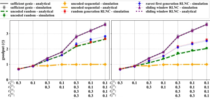
Fig. 7. Goodput for sparse moving (left) and strict moving (right) window for sources N∈ {1,2,4}, RTTκc=3, window size w=24, generation sizeg=12 and burst rater=0.3.

a) Per source count: Increasing the number of sources increases the overall goodput with both window models. As described in Section IV-B, the maximum goodput for the uncoded sequential approach is η= 1(but it also cannot exceed the goodput of the sufficient genie). The uncoded sequential already approaches its theoretical maximum η= 1 goodput in case of using only N = 2 sources.

In the case of uncoded random and the rateless RNLC coded approaches, the number of duplicates increases with the number of sources. Therefore, these protocols cannot achieve the goodput of thesufficient geniefor sourcesN ≥ 2. Using sparse moving window, the performances of uncoded random and rateless RNLC coded approaches follow similar trends. In contrast to that, using a strict moving window to restrict the network delay, uncoded random approach has a significant goodput drop compared to the rateless RNLC coded approach. These results show that RLNC coding can decrease the packet delay in a multi-source network (or increase the goodput, while having the same delay constraints as the uncoded random). Our results suggest that we can achieve optimal goodput by using RLNC coded sliding window approach.

b) Per window size: Fig. 8 shows the impact of the window size on the goodput. Sufficient genieand thecoded sliding windowhave the achievable maximum goodput that is independent of