Comparison of single and ensemble-based convolutional neural networks for cancerous
image classification
Oktavian Lantang
a, Gyorgy Terdik
a, Andras Hajdu
b, Attila Tiba
baDepartment of Applied Information Technology and its Theoretical Background, University of Debrecen
oktavian_lantang@unsrat.ac.id terdik.gyorgy@inf.unideb.hu
bDepartment of Computer Graphics and Image Processing, University of Debrecen
hajdu.andras@inf.unideb.hu tiba.attila@inf.unideb.hu
Submitted: June 16, 2020 Accepted: March 17, 2021 Published online: March 31, 2021
Abstract
In this work, we investigated the ability of several Convolutional Neural Network (CNN) models for predicting the spread of cancer using medical images. We used a dataset released by the Kaggle, namely PatchCamelyon.
The dataset consists of 220,025 pathology images digitized by a tissue scanner.
A clinical expert labeled each image as cancerous or non-cancerous. We used 70% of the images as a training set and 30% of them as a validation set. We design three models based on three commonly used modules: VGG, Inception, and Residual Network (ResNet), to develop an ensemble model and implement a voting system to determine the final decision. Then, we compared the performance of this ensemble model to the performance of each single model. Additionally, we used a weighted majority voting system, where the final prediction is equal to the weighted average of the prediction produced by each network. Our results show that the classification of the two ensemble models reaches 96%. Thus these results prove that the ensemble model outperforms single network architectures.
doi: https://doi.org/10.33039/ami.2021.03.013 url: https://ami.uni-eszterhazy.hu
45
Keywords:Cancer image classification, ensemble-based model, convolutional neural network.
1. Introduction
Currently, non-communicable diseases are the most significant contributor to mor- tality rates throughout the world. One type of non-communicable disease that plays an essential role in the high number of deaths is cancer. In 2015 WHO es- timated that cancer was the leading cause of human death during the productive period, which is below 70 years [2]. By definition, cancer refers to more than one hundred types of diseases with their unique features. Every human being has tril- lions of body cells that multiply and depend on each other. The body’s metabolism automatically controls the development of each cell to maintain its size and shape.
However, cancer cells work oppositely. These cells develop regardless the protocol instructed by the human body. And worse, cancer cells can move from one place to another [21].
In the last decade, pathologists used a microscope to predict cancer. Experts are trained to understand clinical symptoms and later diagnose them. The doctor uses these results for decision making. Now routines like this are no longer a priority since the development of the whole slide image scanner documents of the histological images in digital form. By relying on sophisticated imaging and analysis techniques, this tool can record more complex variables that exist in histological images [12]. Furthermore, the images produced by this tool can detect not only the presence of cancer cells in the body but also show biological processes such as apoptosis, angiogenesis, and metastasis [22]. The histological image documentation process massively produces a tremendous amount of data. The availability of a large amount of data can be seen as an opportunity to develop a machine learning system by designing a Convolutional Neural Network (CNN) [17].
The success of CNNs in producing good predictions can be seen in many pre- vious works, among others [7, 11, 18, 19]. Krizhevsky et al. developed a network called Alexnet. This network is designed in eight stack layers. The eight layers are divided into two large blocks, and the first is filled by five convolutional layers and three fully connected layers. While at the last layer, this model has a 1000-way softmax, which refers to multiclass classification problems. They trained it with 1.2 million high-resolution images provided by ImageNet. Using this model, a 16.4%
error rate for 5 CNN architectures and a 15.3% error rate for 7 CNN ones in the top five classifications were reported [11].
The VGG module was developed by Simonyan et al. The idea of this network is the definition and the repetition of convolutions blocks. This model also utilizes Max Pooling layers to reduce the dimension and small filter to decrease computation costs. Satisfactory results were reported in this work. Namely, using the same dataset, this study reports a 6.8% error rate for the top five predicted labels and a 23.7% error rate in the top first predicted labels [18].
As we know, CNN is an architecture that was developed to extract features from
images comprehensively. However, one of the problems faced is the high variety of the spatial position of the image information. In a dataset, the information we want to retrieve is not always in the center of the image. Moreover, the desired information may have a small percentage of other details. The large spatial variety of information from an image makes it difficult to determine the suitable filter size for CNN. Using a large filter makes the information more global, thus increasing the cost of computing. On the other hand, if we use a small filter, it will cause the information to be more local and eliminate essential knowledge from the image. For this reason, the Inception architecture was designed by installing multiple different size filters at the same level and concatenate them to reduce computing costs without losing deciding information. This idea will produce architectures that tend to be broad than deep [19].
The above studies showed that a deeper and more complex architecture resulted in a better accuracy and validation score. However, deep and complex architecture can damage the accuracy and validation of the model. He et al. tried to solve this problem by developing a Residual Network (Resnet) model. Resnet’s basic concept is to group CNN into several blocks, and each block has a short cut to do a pass. This model architecture is constructed from 34 layers of residual blocks for the smallest architecture to 152 layers for the most complex one. The 152 layers single architecture reported very satisfying results by having a 19.38% error rate for the top first predicted labels and a 4.49% error rate for the top five predicted labels [7].
2. Related works
Classification using deep learning methods has produced excellent works. One of these was the work of Veeling et al. [20]. The suggested model adopts the DenseNet architecture, which uses Dense Block and Transition Block. Dataset was tested on six different single DenseNet models, and the P4M-DenseNet model gave the best results with an accuracy score of 89.8%. Kassani et al. [10] developed a model from three base modules: VGG19, MobileNet, and DenseNet. The model was trained using transfer learning techniques in a CNN ensemble framework utilizing four different datasets, including the PatchCamelyon dataset. Specifically, on the PatchCamelyon dataset, this work reported the accuracy of 94.64% for the CNN ensemble model. Another study from Xia et al. [23] compared two well-known CNN training methods, namely training from scratch and fine-tuning. They used the Camelyon 16 dataset, which is the origin of the PatchCam dataset. This work reported a result of 84.3% accuracy when the GoogleLeNet architecture was trained using a fine-tuned training method.
In this work, we investigated two CNN models’ ability, namely single and en- semble, for predicting the spread of cancer using medical images. We used a Patch- Camelyon dataset of 220,025 pathology images digitized using a tissue scanner and labeled as cancerous or non-cancerous. 70% of images were used as a training set and the rest as the validation set. To develop an ensemble model, we chose three
commonly used CNN modules, namely VGG, Inception, and Residual ResNet, with a voting system to determine the final decision. Furtherly, we compared the performance of this ensemble model to the performance of each single module. Ad- ditionally, we used a weighted majority voting system where the final prediction is equal to the weighted average of the prediction produced by each network.
3. Methodology
3.1. Dataset, hardware and software
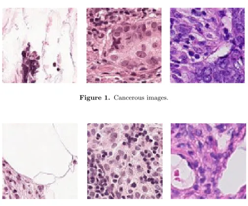
The data we use is published in Kaggle, the PatchCamelyon dataset, which is derived from the Camelyon16 Dataset [1, 20]. The dataset consists of pathology images generated from a digital scanner. The whole slide image are broken down into smaller segments of size92×92pixels. The dataset contains 220,025 images, then divided 154,018 for the training set and 66,007 for the validation set. To simplify our work, we use a validation set as well as a test set. Next, we show sample images of the data set in Figures 1 and 2. To support this work, we utilize Google Collaboraty with NVIDIA Cuda Compilation Tool V8.0.61 besides that we also use DELL desktop with GEFORCE GTX 1060 6GB.
Figure 1. Cancerous images.
Figure 2. Non-cancerous images.
3.2. Preprocessing and augmentation
We chose 92×92pixels as the input size. Furthermore, we used an augmentation process as part of image pre-processing to provide a sufficient amount of data and resist the overfitting condition. The technical process involved rotation, shifting, shearing, zoom and flipping as shown in Table 1.
Table 1. Augmentation process.
Rotation 45∘ Shifting 0.2 Shearing 0.2
Zoom 0.2
Flipping Horizontal
3.3. Base model of ensembles
As for the neural network architectures VGG, Inception, ResNet, we did not in- tegrate any existing realizations, we implemented them from scratch to gain less complex models. The first model was the LT-VGG based on the VGG module. We stacked thirteen layers with the following details: ten convolutions layers and three fully connected ones. We inserted a Max Pooling layer after every two convolutions layers to have four pooling layers in total. Before entering fully connected layers, the feature dimensions are changed using the Flatten layer and then passed on to three fully connected layers: two 64-neurons and a Softmax with two-classes at the end of the network.
The second model was LT-Inception based on the Inception module. The mod- ifications performed in this model include twelve convolutions, which are divided into two levels. Each level is filled by six convolutions and one Max Pooling layer.
Before going to the next level, the convolutions at level one were concatenated.
After the concatenation process at the second level, the dimension was shrunk us- ing the Average Pooling layer. The dimensions were changed using the Flatten layer and finally streamed to three fully connected layers of two 64-neurons and a Softmax for two-classes.
The last model was the LT-ResNet based on the ResNet module. We installed eighteen convolutions layers and also inserted one residual layer for every three convolutional layers. So in total, we used 24 convolutions layers. We also used the Average Pooling layer to reduce the features’ dimensions before converting to one dimension using the Flatten Layer. Next, we used two fully connected layers of two 64-neurons and a Softmax two-classes.
Refers to [4, 15], Softmax function 𝑓(𝑠) :R𝐾 → R𝐾 is a vector function in the range [0,1], where 𝐾 is the number of classes. This function is obtained by calculating the exponential number to the power of𝑠𝑖, where𝑠𝑖 refers to the score 𝑠 from class𝑖. Hereafter, numerator divided by the sum of the constant𝑒 to the
power of all score in number of classes:
𝑓(𝑠)𝑖= 𝑒𝑠𝑖
∑︀𝐾
𝑐=1𝑒𝑠𝑐. (3.1)
3.4. Ensemble model architecture
The ensemble method is one of the popular techniques to improve CNN’s accu- racy, as described in [9]. The CNN ensemble technique is a combination of several CNNs used to accomplish the same task. In their study, 193 articles were selected in four different databases: ACM, Scopus, IEEE Xplore, and PubMed. Their work reported that the majority voting method is the most widely used in the heterogeneous ensemble type. The most popular type of classifier is Support Vec- tor Machine, beating Artificial Neural Network in fourth place. Nevertheless, the dataset used is mostly extracted from mammograms, not images.
To see more clearly the use of the CNN ensemble method in image datasets, we also studied the work of Savelli et al. [16]. By implementing the CNN Ensemble, they detected minor lesions in medical images. From this work, we can see how the four CNN singles are combined, and then the final decision is taken from the average score of the four single models. This work used the dataset of medical images, namely INbreast, which relates to breast cancer, and E-ophtha, a retinal fundus image.
Furthermore, Haragi’s work[6] designed the CNN ensemble for the classification of skin lesions. In this study, we focus on recognizing how the final decision tech- niques are applied to the ensemble method. We can see that the authors consider several ways, such as Probabilistic, Majority Voting, and Weighting. From the results reported, there is a significant difference in accuracy between single CNN and ensemble one. Meanwhile, ensemble CNN’s final decision technique shows that Simple Majority Voting provides the best accuracy score. On the other hand, the weighting method excels in measuring the area under curve (AUC).
We trained three base models separately so that the ensemble model will have three prediction results. We chose two types of voting systems that are used by the ensemble model. The first voting system is majority voting. This system gives each base model equal weight without considering achieving each model’s accuracy when trained separately. Whereas the other voting system is that we apply special weights to each model, referring to the accuracy of each training’s results. Furtherly, we compared the performance of this ensemble model to the performance of each single model. The architecture of the ensemble model shown in Figure 3.
3.5. Training process
We experimented by gradually increasing the epoch from 10 to 100. The best results were obtained at the epoch of 50. After that, there was an inconsistency in both machine capability and the accuracy score. To save training time, we took
Figure 3. Achitecture of the ensemble model.
advantage of implementing the batch size system in the training process.
Since we used more than eight convolutions with non-linear activation, we de- cided to use the Normal Distribution developed by He et al. [8] as initial weights during the training process. To optimize the training process, we took advantage of the ADAM optimizer by setting the learning rate at 1e-4 and reduce by 1e-6 for each subsequent epoch.
To measure the performance of the model, we have calculated its accuracy, precision and recall score [3, 14]. It can be derived using the following formulas:
Accuracy= TP TP+FP, Precision= TP+TN
TP+TN+FP+FN, Recall= TP
TP+FN,
where TP stands for true positive, and this value was taken from the data in class 0 (no cancer) and predicted to be accurate as class 0. TN is for true negative, that is, data was on class 1 (cancer) and correctly predicted as a member of class 1.
Conversely, FP is an abbreviation of false positive, where FP is a member of class
1, which is wrongly predicted as a member of class 0. And lastly, FN is for false negative, which is a member of class 0 that was wrongly predicted as a member of class 1.
We also measured the loss score that represents how far the model is from the target. To calculate the loss score, we used the cross-entropy for the Softmax loss function with two classes target. By having formula (3.1), the softmax loss function will become:
CE=−
∑︁𝐾
𝑖
𝑡𝑖log(𝑓(𝑠)𝑖). (3.2) Equation (3.2) explains that cross-entropy CE is the sum of ground truth 𝑡𝑖 loga- rithm the CNN score of each class that represents by𝑓(𝑠)𝑖.
The ensemble process is to train the three models separately, then we vote. The first type of voting used is simple majority voting. Here, we do not pay attention to each model’s achievement in the training process. In other words, each model gets the same portion in the voting process. The second type of voting is that we provide different portions for each model. We tried some combinations of weights considering the individual accuracies of the ensemble members. The results show that an optimal choice of weights is 0.35 for the two best networks and 0.3 for the third network. So, we set LT-ResNet and LT-VGG having weights 0.35 and LT-Inception 0.30. Voting system itself refers to [5, 13], if we have multiple scores 𝑥1, 𝑥2, . . . , 𝑥𝑛, with corresponding weights𝑤1, 𝑤2, . . . , 𝑤𝑛, then the weighted mean can be calculated through
¯ 𝑥=
∑︀𝑛 𝑖=1𝑤𝑖𝑥𝑖
∑︀𝑛 𝑖=1𝑤𝑖
.
4. Results
4.1. Loss score
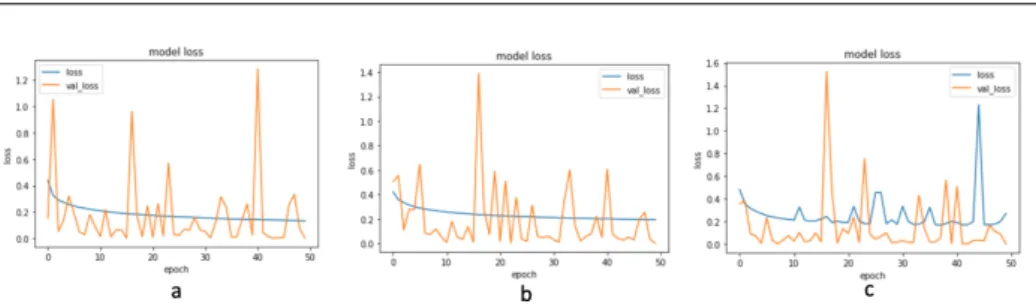
Figure 4 illustrates the loss score of the three models while training. Graph 𝑎 shows that the LT-ResNet model’s loss score has a stable movement, likewise in graph𝑏, which displays a decrease in the loss score, which is also stable from the LT- Inception model. Meanwhile, the LT-VGG model shows the unsteady movement of reducing the loss score, as shown in graph𝑐. Figure 4 shows the three models’ loss scores, respectively, LT-ResNet 0.1324, LT-Inception 0.1937, and LT-VGG 0.2689 at the last epoch.
4.2. Accuracy, precision and recall
Figure 5 describes the training process of the three base models. From this figure, we can see the accuracy and validation score of the models. These three graphs show a significant increase in accuracy from the first epoch to the 50 epochs. The con- sistently smaller differences between the training and validation accuracies (blue,
Figure 4. Loss of: (a) LT-ResNet, (b) LT-Inception, (c) LT-VGG.
yellow lines on Figure 5, respectively) prove that the model is not overfitting. The performance of the LT-ResNet model is shown in graph𝑎, with an accuracy score of 0.95. Meanwhile, the LT-Inception model’s performance is shown in graph𝑏, with an accuracy score of 0.93. The LT-VGG model also has a good performance, as shown in graph𝑐, with an accuracy score of 0.95. The training process’s complete results, which include the accuracy, precision, and recall scores of the three models, are presented in Table 2.
Figure 5. Accuracy of: (a) LT-Resnet, (b) LT-Inception, (c) LT-VGG.
Table 2. Precision, Recall and Accuracy of the investigated models.
𝑥 LT-ResNet LT-Inception LT-VGG MV WMV
Pre 0 0.95 0.92 0.95 0.95 0.95
Rec 0 0.97 0.96 0.97 0.98 0.98
Pre 1 0.95 0.93 0.96 0.96 0.96
Rec 1 0.92 0.89 0.92 0.93 0.93
Acc 0.95 0.93 0.95 0.96 0.96
After getting the results from these three models, we proceed by using the voting method as an implementation of the ensemble model. The majority voting (MV) results and the weighted majority voting (WMV) results show an equivalent quality in the calculation of each class. We have precision scores of 0.95 and 0.96,
respectively, for Class 0 and Class 1. Recall scores apiece 0.98 and 0.93 for Class 0 and Class 1. Finally accuracy score of these two voting systems corrects the accuracy value of all single models, which is 0.96 for both class.
4.3. Confusion matrix
To see the performance of the models, we present their predictions on the validation set. In Table 3, we report the predicted results of the three base models and two voting systems.
Table 3. Confusion matrix of the investigated models.
𝑥 LT-ResNet LT-Inception LT-VGG MV WMV
TP 38043 37657 38186 38392 38397
TN 24677 23634 24504 24773 24787
FP 2020 3063 2193 1924 1910
FN 1265 1653 1124 918 913
From Table 3, we can see that if we compare the prediction results of the three base models, LT-ResNet model is superior in predicting class 1 and LT-VGG model in class 0. However, the ensemble model corrects the achievement of the three base models of around 200 to 300 images per class. Overall, the weighted majority voitng shows the best result with 38,397 images accurately predicted as class 0 and 24,787 images correctly predicted as class 1. On the other hand, there were 1910 images from class 1 that were mistakenly predicted as class 0, and only 913 images in class 0 were incorrectly predicted as members of class 1.
5. Conclusion
From this study, we can conclude that the ensemble method can be used to improve the model’s accuracy. It can be seen from the work of Kassani and ours compared to Veeling and Xia’s works in Table 4. In this case, we experienced that the weighting method had no significant impact on the voting process. It can be seen from the equal accuracy score for the two ensemble models. Developing a network from scratch can be leveraged to reduce the complexity and depth of the architecture without compromising the network’s quality. This can be seen from the comparison of the accuracy of our work with Kassani’s.
From some of our references, several methods might be considered to be used in future work. One of them is the hyperparameter tuning method. The grid search method seems considerable to determine hyperparameters automatically.
However, considering machine capability, we cannot use it at this time, and instead, we specify the parameters manually. Another thing that can be considered is the weighting method for the final decision, which can be part of the training
parameters. In other words, the user does not need to determine the weight of each single model, but the training process itself determines which model has the most influence on the ensemble model.
Table 4. Comparison results.
Method Architecture Accuracy
Veeling et al. P4M-DenseNet 89.8%
Xia et al. GoogleLeNet fine-tuned 84.3%
Kassani et al Ensemble 94.64%
Proposed method Ensemble 96%
Acknowledgments. This work was supported in part by the project EFOP- 3.6.3-VEKOP-16-2017-00002, supported by the European Union, co-financed by the European Social Fund. Research was also supported by the ÚNKP-19-3–I.
New National Excellence Program of the Ministry for Innovation and Technology.
This study was funded by LPDP Indonesia in the form of a doctoral scholarship (https://www.lpdp.kemenkeu.go.id)
References
[1] B. E. Bejnordi,M. Veta,P. J. van Diest,B. van Ginneken,N. Karssemeijer,G.
Litjens,J. A. W. M. van der Laak, theCAMELYON16 Consortium:Diagnostic As- sessment of Deep Learning Algorithms for Detection of Lymph Node Metastases in Women With Breast Cancer, JAMA 318.22 (2017), pp. 2199–2210,
doi:https://doi.org/10.1001/jama.2017.14585.
[2] F. Bray,J. Ferlay,I. Soerjomataram,R. Siegel,L. Torre,A. Jemal:Global Can- cer Statistics 2018: GLOBOCAN Estimates of Incidence and Mortality Worldwide for 36 Cancers in 185 Countries, CA: A Cancer Journal For Clinicians 68.6 (2018), pp. 394–424, doi:https://doi.org/10.3322/caac.21492.
[3] T. Fawcett:An Introduction to ROC Analysis, Pattern Recognition Letters 27.8 (2006), pp. 861–874,
doi:https://doi.org/10.1016/j.patrec.2005.10.010.
[4] I. Goodfellow,Y. Bengio,A. Courville:Deep Feedforward Networks, in: Deep Learn- ing, USA: MIT press, 2016, p. 181.
[5] J. Grossman,M. Grossman,R. Katz, in: The First System of Weighted Differential and Integral Calculus, Non-Newtonian Calculus, 2006.
[6] B. Harangi:Skin Lesion classification With Ensemble of Deep Convolutional Neural Net- works, Journal of Biomedical Informatics 86 (2018), pp. 25–32,
doi:https://doi.org/10.1016/j.jbi.2018.08.006.
[7] K. He,X. Zhang,S. Ren, J. Sun:Deep Residual Learning for Image Recognition, in:
Proceedings of the 2016 IEEE Conference on Computer Vision and Pattern Recognition, Las Vegas, NV, USA: IEEE, 2016, pp. 770–778,
doi:https://doi.org/10.1109/CVPR.2016.90.
[8] K. He, X. Zhang, S. Ren,J. Sun:Delving Deep Into Rectifiers: Surpassing Human- Level Performance On Imagenet Classification, in: Proceedings of the IEEE international conference on computer vision, Santiago,Chile: IEEE, 2015, pp. 1026–1034,
doi:https://doi:10.1109/ICCV.2015.123.
[9] M. Hosni,I. Abnane,A. Idri,J. M. C. de Gea,J. L. F. Aleman:Reviewing Ensemble Classification Methods in Breast Cancer, Computer Methods and Programs in Biomedicine 177 (2019), pp. 89–112,
doi:https://doi.org/10.1016/j.cmpb.2019.05.019.
[10] S. H. Kassani, P. H. Kassani,M. J. Wesolowski,K. A. Schneider,R. Deters:
Classification of Hispatology Biopsy Images Using Ensemble of Deep Learning Networks, arXiv preprint arXiv:1909.11870 (2019).
[11] A. Krizhevsky,I. Sutskever,G. Hinton:ImageNet Classification with Deep Convolu- tional Neural Networks, Communications of the ACM 60.6 (2017), pp. 1079–1105,
doi:https://doi.org/10.1145/3065386.
[12] A. Madabhushi:Digital Pathology Image Analysis: Opportunities and Challenges, Imaging In medicine 1.1 (2009), pp. 7–10.
[13] R. Mesiar, J. Spirkova: Weighted Means and Weighting Functions, Kybernetika 42.2 (2006), pp. 151–160.
[14] D. M. W. Powers:Evaluation: From Precision, Recall and F-measure to ROC, Informed- ness, Markedness and Correlation, Journal of Machine Learning Technologies 2.1 (2011), pp. 37–63,
doi:https://doi.org/10.9735/2229-3981.
[15] P. Sadowski:Notes on back propagation(2016), url:https://www.ics.uci.edu/pjsadows/notes.pdf.
[16] B. Savelli,A. Bria,M. Molinara,C. Marrocco,F. Tortorella:A Multi-context CNN Ensemble For Small Lesion Detection, Artificial Intelligence in Medicine 103 (2020), pp. 1–13,
doi:https://doi.org/10.1016/j.artmed.2019.101749.
[17] H.-C. Shin,H. Roth,M. Gao,L. Lu, Z. Xu,I. Nogues,J. Yao, D. Mollura,R.
Summers:Deep Convolutional Neural Networks for Computer-Aided Detection: CNN Ar- chitectures, Dataset Characteristics and Transfer Learning, IEEE Transactions on Medical Imaging 35.5 (2016), pp. 1285–1298,
doi:https://doi.org/10.1109/tmi.2016.2528162.
[18] K. Simonyan,A. Zisserman:Very Deep Convolutional Networks for Large-Scale Image Recognition, arXiv preprint arXiv:1409.1556.
[19] C. Szegedy,W. Liu,Y. Jia,Y. Jia,S. Reed,D. Anguelov,D. Erhan,V. Vanhoucke, A. Rabinovich:Going Deeper with Convolutions, in: Proceedings of the 2015 IEEE Confer- ence on Computer Vision and Pattern Recognition, Boston, MA, USA: IEEE, 2015, pp. 1–9, doi:https://doi.org/10.1109/cvpr.2015.7298594.
[20] B. S. Veeling,J. Linmans,J. Winkens,T. Cohen,M. Welling:Rotation Equivariant CNNs for Digital Pathology, in: Proceedings on the 2018 Medical Image Computing and Computer Assisted Intervention, Spring, Cham, 2018, pp. 210–218,
doi:https://doi.org/10.1007/978-3-030-00934-2_24.
[21] R. Weinberg:How Cancer Arises, Scientific American 275.3 (1996), pp. 67–70.
[22] R. Weissleder:Molecular Imaging in Cancer, Science 312.5777 (2006), pp. 1168–1171, doi:https://doi.org/10.1126/science.1125949.
[23] T. Xia,A. Kumar,D. Feng,J. Kim:Patch-level Tumor Classification in Digital His- patology Images with Domain Adapted Deep Learning, in: 2018 40th Annual International Conference of the IEEE Engineering in Medicine and Biology Society (EMBC), Honolulu, HI, USA: IEEE, 2018, pp. 644–647,
doi:https://doi:10.1109/EMBC.2018.8512353.