Combining predictive distributions for statistical post-processing of ensemble forecasts

post-processing of ensemble forecasts

S´ andor Baran

and Sebastian Lerch

1

Faculty of Informatics, University of Debrecen Kassai ´ ut 26, H-4028 Debrecen, Hungary

2

Heidelberg Institute for Theoretical Studies

Schloss-Wolfsbrunnenweg 35, D-69118 Heidelberg, Germany

3

Institute for Stochastics, Karlsruhe Institute of Technology, Englerstraße 2, D-76128 Karlsruhe, Germany

July 14, 2017

Abstract

Statistical post-processing techniques are now widely used to correct systematic biases and errors in calibration of ensemble forecasts obtained from multiple runs of numerical weather prediction models. A standard approach is the ensemble model output statistics (EMOS) method, a distributional regression approach where the fore- cast distribution is given by a single parametric law with parameters depending on the ensemble members. Choosing an appropriate parametric family for the weather variable of interest is a critical, however, often non-trivial task, and has been the focus of much recent research. In this article, we assess the merits of combining predictive distributions from multiple EMOS models based on different parametric families. In four case studies with wind speed and precipitation forecasts from two ensemble pre- diction systems, we study whether state of the art forecast combination methods are able to improve forecast skill.

Key words: ensemble model output statistics, ensemble post-processing, forecast com- bination, precipitation, probabilistic forecasting, wind speed.

1

arXiv:1607.08096v3 [stat.ME] 13 Jul 2017

1 Introduction

Nowadays, weather forecasts are typically based on the output of numerical weather predic- tion (NWP) models which describe the dynamical and physical behavior of the atmosphere through nonlinear partial differential equations. Single deterministic predictions produced by single runs of such models fail to account for uncertainties in the initial conditions and the numerical model. Therefore, NWP models are nowadays typically run several times with varying initial conditions and model physics, resulting in an ensemble of forecasts, see Palmer (2002) and Gneiting and Raftery (2005) for reviews. Examples of ensemble pre- diction systems (EPSs) are the 51-member European Centre for Medium-Range Weather Forecasts (ECMWF) ensemble (Molteni et al., 1996), the eight-member University of Wash- ington Mesoscale ensemble (UWME; Eckel and Mass, 2005), and the 11-member Aire Limit´ee Adaptation dynamique D´eveloppement International-Hungary Ensemble Prediction System (ALADIN-HUNEPS; Hor´anyi et al., 2006) of the Hungarian Meteorological Service (HMS).

The transition from single deterministic forecasts to ensemble predictions can be seen as an important step towards probabilistic forecasting, however, ensemble forecasts are often underdispersive and subject to systematic bias. They thus require some form of statistical post-processing.

Over the past decade, various statistical post-processing methods have been proposed in the meteorological literature. In the Bayesian model averaging (BMA; Raftery et al., 2005) approach the forecast distribution is given by a weighted mixture of parametric densities, each of which depends on a single ensemble member with mixture weights being determined by the performance of the ensemble members in the training period. Within this article we build on the conceptually simpler ensemble model output statistics (EMOS) approach pro- posed by Gneiting et al. (2005), where the conditional distribution of the weather variable of interest given the ensemble predictions is modeled by a single parametric family. The pa- rameters of the forecast distribution are connected to the ensemble forecast through suitable link functions. For example, the original EMOS approach models temperature with a Gaus- sian predictive distribution where the mean is an affine function of the ensemble member forecasts, and the variance is an affine function of the ensemble variance.

Over the last years the EMOS approach has been extended to other weather variables such as wind speed (Thorarinsdottir and Gneiting, 2010; Lerch and Thorarinsdottir, 2013; Baran and Lerch, 2015; Scheuerer and M¨oller, 2015), precipitation (Scheuerer, 2014; Scheuerer and Hamill, 2015; Baran and Nemoda, 2016), and total cloud cover (Hemri et al., 2016). The success of statistical post-processing relies on finding appropriate parametric families for the weather variable of interest. However, the choice of a suitable parametric model is a non- trivial task and often a multitude of competing models is available. The relative performance of these models usually varies for different data sets and applications.

Regime-switching combination models proposed by Lerch and Thorarinsdottir (2013) partly alleviate the limited flexibility of single parametric family models by selecting one of

several candidate models based on covariate information. However, the applicability of this approach is subject to the availability of suitable covariates. For some weather variables, full mixture EMOS models can be formulated where the parameters and weights of a mixture of two forecast distributions are jointly estimated (Baran and Lerch, 2016). However, such approaches are limited to specific weather variables, and the estimation is computationally demanding.

In this article we investigate the feasibility of another, more generally applicable route towards improving the forecast performance that has recently received some interest, and has for example been suggested in Yang et al. (2017). Motivated by promising results of M¨oller and Groß (2016) and Bassetti et al. (2017), we study whether combining predictive distributions from individual post-processing models is able to significantly improve the forecast performance. In a first step, individual EMOS models based on single parametric distributions are estimated. In a second step the forecast distributions are combined utilizing state of the art forecast combination techniques such as the (spread-adjusted) linear pool, the beta-transformed linear pool (Gneiting and Ranjan, 2013), and a recently proposed Bayesian, essentially non-parametric calibration approach (Bassetti et al., 2017). Further, we propose a computationally efficient ’plug-in’ approach to determining combination weights in the linear pool that is specific to post-processing applications.

The remainder of this article is organized as follows. Section 2 contains a description of the ensembles and the observation data. In Section 3, the EMOS method is reviewed, and the individual EMOS models for wind speed and precipitation are introduced. Thereafter, Section 4 provides a description of the forecast combination approaches and the application to post-processing. The various EMOS models and forecast combination approaches are compared in four case studies in Section 5. The article concludes with a discussion in Section 6.

2 Data

We consider two different weather variables, wind speed and precipitation accumulation, and two distinct data sets of ensemble forecasts and corresponding validating observations for each weather quantity. The wind speed data sets are identical to data used in Baran and Lerch (2015, 2016), whereas the precipitation data coincide with those studied in Baran and Nemoda (2016). For detailed descriptions of the ensemble forecasts and corresponding observations we refer to these articles and references therein.

Ensemble members that are generated with the help of random perturbations of initial conditions are statistically indistinguishable, and are referred to as exchangeable. The notion of exchangeability of ensemble members is important for the formulation of post-processing models, see Section 3 for details.

2.1 University of Washington mesoscale ensemble

The UWME covers the Pacific Northwest region of North America with a horizontal resolu- tion of 12 km and consists of eight members generated from different runs of the fifth gen- eration Pennsylvania State University–National Center for Atmospheric Research mesoscale model (Grell et al., 1995). The initial and boundary conditions of the model runs are provided by different sources, the individual ensemble members can therefore be clearly dis- tinguished and are considered to be non-exchangeable. The data set at hand contains 48 h ahead forecasts and corresponding validating observations for 10 m maximal wind speed (given in m/s) and 24 h precipitation accumulation (given in mm) for 152 stations in the Automated Surface Observing Network (National Weather Service, 1998) in the U.S. states of Washington, Oregon, Idaho, California and Nevada.

We focus on calendar year 2008 with additional forecasts and observations from the last months of 2007 used to allow for training periods of equal length for the model estimation.

After removing days and locations with missing predictions and/or observations, stations where data are available only on very few days are also removed resulting in 101 stations with 27 481 individual forecast cases for wind speed and 75 stations with 20 448 individual forecast cases for precipitation.

2.2 ALADIN-HUNEPS ensemble

The ALADIN-HUNEPS system covers large parts of continental Europe on an 8 km grid.

It is obtained with dynamical downscaling of the global ARPEGE based PEARP system of M´et´eo France (Hor´anyi et al., 2011; Descamps et al., 2015) and consists of 11 ensemble members, 10 of which are exchangeable forecasts from perturbed initial conditions, and one of which is a control member from the unperturbed analysis.

We use ensembles of 42 h ahead forecasts of 10 m instantaneous wind speed (in m/s) and 24 h precipitation accumulation (in mm) issued for 10 major cities in Hungary together with the corresponding validation observations. Wind speed data are available for a one-year period from 1 April 2012 to 31 March 2013, and precipitation data are available between 1 October 2010 and 25 March 2011. Days with missing forecasts and/or observations are excluded from the analysis for both wind speed (6 days) and precipitation (2 days).

3 Ensemble model output statistics

Successful statistical post-processing of ensemble forecasts relies on finding and estimating appropriate parametric models for the conditional distribution of the weather variable of interest given the ensemble predictions. In case of the EMOS approach, the forecast dis- tribution is given by a single parametric law with parameters depending on the ensemble

forecast. While temperature can be modeled by a normal distribution (Gneiting et al., 2005), the choice of a suitable parametric family is much less straightforward for weather variables such as wind speed or precipitation. A multitude of post-processing approaches and model- ing strategies has been proposed over the last years. In the following short review, we focus on EMOS models for wind speed and precipitation, and subsequently investigate methods to combine forecast distributions from different models.

3.1 EMOS models for wind speed

Non-negative weather variables such as wind speed require skewed predictive distributions with non-negative support like Weibull (Justus et al., 1978) or gamma distributions (Garcia et al., 1988). Recently developed EMOS approaches utilize truncated normal (TN; Tho- rarinsdottir and Gneiting, 2010), gamma (Scheuerer and M¨oller, 2015), generalized extreme value (GEV; Lerch and Thorarinsdottir, 2013) and log-normal (LN; Baran and Lerch, 2015) distributions to model the conditional distribution of wind speed given the ensemble predic- tions. Here, we focus on the truncated normal and log-normal model.

3.1.1 Truncated normal EMOS model We denote by N₀ µ, σ²

the TN distribution with location µ, scale σ > 0, and cut-off at zero with probability density function (PDF)

g(x|µ, σ) :=

1

σϕ (x−µ)/σ

Φ µ/σ , if x≥0, and g(x|µ, σ) := 0, otherwise, where ϕ and Φ are the PDF and the cumulative distribution function (CDF) of the standard normal distribution, respectively. The predictive distribution of the EMOS model proposed by Thorarinsdottir and Gneiting (2010) is

N₀ a₀+a₁f₁+· · ·+a_Kf_K, b₀+b₁S²

with S² := 1 K−1

K

X

k=1

f_k−f2

, (3.1) where f₁, f₂, . . . , f_K denote the ensemble of distinguishable forecasts of wind speed for a given location and time, and f is the ensemble mean. Location parameters a₀, a₁, . . . , a_K ∈ R and scale parameters b₀ ∈R, b₁ ≥0 of model (3.1) can be estimated from the training data, consisting of ensemble members and verifying observations from the preceding n days, by optimizing an appropriate verification score, see Section 3.3.

However, most operational EPSs generate forecasts using random perturbations of the initial conditions resulting in statistically indistinguishable ensemble members which are re- ferred to as exchangeable. Examples include the 51-member ECMWF ensemble, as well as sub-ensembles of forecasts from single models that form groups of exchangeable mem- bers within multi-model EPSs such as the THORPEX Interactive Grand Global Ensemble

(Swinbank et al., 2016) or the GLAMEPS ensemble (Iversen et al., 2011). To account for the generation of the forecasts, ensemble members within a given group of exchangeable mem- bers should share the same coefficients in the post-processing model (Fraley et al., 2010;

Gneiting, 2014).

To formalize this notion, a generalized formulation of model (3.1) for the case of M ensemble members divided into K groups, where the kth group contains M_k ≥ 1 exchangeable ensemble members (PK

k=1M_k = M) introduced in Baran and Lerch (2015) is given by

N0

a0+a1 M1

X

`1=1

f1,`1 +· · ·+aK MK

X

`K=1

fK,`_K, b0+b1S²

.

Analogous concepts apply to all EMOS models discussed in the subsequent sections.

3.1.2 Log-normal EMOS model

As an alternative to the TN EMOS model, Baran and Lerch (2015) introduce an EMOS approach based on log-normal forecast distributions where the mean m and variance v of the predictive distribution are linked to the ensemble members as

m =α₀+α₁f₁+· · ·+α_Kf_K and v =β₀+β₁S². (3.2) These quantities uniquely determine the location µ and shape σ > 0 of the underlying LN distribution LN µ, σ

with PDF h(x|µ, σ) := 1

xσϕ (logx−µ)/σ

, if x≥0, and h(x|µ, σ) := 0, otherwise, via transformations

µ= log

m²

√v+m²

and σ =

r log

1 + v m²

.

Similar to the TN EMOS model, estimates of parameters α₀, α₁, . . . , α_K ∈ R and β₀ ∈ R, β₁ ≥0 are obtained by optimizing the mean of an appropriate verification score over all forecast cases in the training data.

3.1.3 Combination and mixture models

The TN and LN models described above model the conditional distribution of wind speed given the ensemble predictions with a single parametric forecast distribution. This approach relies on the choice of a suitable parametric family, and limits the flexibility of the model. For instance, it can be demonstrated that the heavier tails of the LN model are more appropriate for modeling higher wind speeds in the right tail of the distribution, whereas the TN model is more appropriate for the bulk of the distribution, see Baran and Lerch (2016) for details.

Therefore, different combination and mixture models have been proposed in the literature.

In the regime-switching combination approach (Lerch and Thorarinsdottir, 2013; Baran and Lerch, 2015) one of the candidate models is selected based on covariate information with suitably adapted parameter estimation procedures. For example, a TN model can be used if the median ensemble forecast is below a threshold η, and an LN model is used in case of median ensemble forecasts exceeding this threshold. Such combination models have been demonstrated to improve the predictive performance compared to the individual models, however, they require the choice of a suitable covariate, and the threshold parameter η has to be determined by repeating the model estimation over a grid of potential values, thereby limiting the flexibility and increasing the computational cost of such approaches.

In order to flexibly combine the advantages of lighter and heavier-tailed distributions and to avoid these problems in the process, Baran and Lerch (2016) propose a mixture model of the form

ψ(x|µ_{T N}, σ_{T N};µ_LN, σ_LN;ω) := ωg(x|µ_{T N}, σ_{T N}) + (1−ω)h(x|µ_LN, σ_LN), (3.3) where the parameters of the component distributions g and h depend on the ensemble forecasts as specified in (3.1) and (3.2). The EMOS coefficients and the weight ω ∈ [0,1]

of the mixture model (3.3) are estimated jointly using optimum score approaches. This mix- ture model approach results in significantly improved calibration (Baran and Lerch, 2016), however, it is computationally very demanding and hinders using standard optimum score estimation based on the continuous ranked probability score due to the lack of an analytic expression of the objective function, see Section 3.3 for details. Similar mixture models where the different component distributions focus on specific regions of interest such as the bulk and the tail above a threshold value have been tested, but models based on truncated normal and generalized Pareto distributions result in worse predictive performance, see Baran and Lerch (2016).

In contrast to the joint estimation of all parameters in (3.3), the forecast combination approaches introduced in Section 4 are two-step procedures where in a first step, EMOS models based on a single parametric family are estimated, and in a second step, these models are combined as a weighted mixture by estimating an appropriate weight. In Section 5 the full mixture model (3.3) is used as a benchmark, whereas the regime-switching combination approach will not be considered any further.

3.2 EMOS models for precipitation

The discrete-continuous nature of precipitation accumulation requires a non-negative predic- tive distribution assigning positive mass to the event of zero precipitation. A popular choice is to consider a continuous distribution that can take both positive and negative values and left censor it at zero (Scheuerer, 2014; Scheuerer and Hamill, 2015; Baran and Nemoda, 2016), which thereby assigns the mass of negative values to zero precipitation accumulation.

3.2.1 Censored and shifted gamma EMOS model

Let G(·|κ, θ) denote the CDF of the Γ(κ, θ) distribution with shape κ > 0 and scale θ > 0 and let δ > 0. Then the CDF of the shifted gamma distribution left censored at zero (CSG) Γ₀(κ, θ, δ) with shape κ, scale θ and shift δ is given by

G₀(x|κ, θ, δ) := G(x+δ|κ, θ), if x≥0, and G₀(x|κ, θ, δ) := 0, otherwise, (3.4) that is, mass G(δ|κ, θ) is assigned to the origin. In the CSG EMOS approach of Baran and Nemoda (2016) the mean m =κθ and variance σ² =κθ² of the uncensored gamma distribution Γ(κ, θ) are affine functions of the ensemble and ensemble mean, respectively, that is

m =a₀+a₁f₁+· · ·+a_Kf_K and σ² =b₀+b₁f . (3.5)

3.2.2 Censored generalized extreme value EMOS model The CDF of a GEV distribution GEV µ, σ, ξ

with location µ, scale σ >0 and shape ξ equals

H(x|µ, σ, ξ) :=





 exp

−

1 +ξ(^x−µ_σ )−1/ξ

, ξ 6= 0;

exp

−exp − ^x−µ_σ

, ξ = 0, if 1 +ξ(x−µ)/σ >0, and zero otherwise, which for −0.278< ξ <1 has a positive skewness and an existing mean

m =

(µ+σ^{Γ(1−ξ)−1}_ξ , ξ6= 0;

µ+σγ, ξ= 0,

where γ denotes the Euler-Mascheroni constant.

The EMOS model for precipitation accumulation proposed by Scheuerer (2014) is based on a censored GEV distribution GEV0 µ, σ, ξ

with CDF

H₀(x|µ, σ, ξ) =H(x|µ, σ, ξ), if x≥0, and H₀(x|µ, σ, ξ) := 0, otherwise, (3.6) where

m=α0+α1f1+· · ·+αKfK+νp0 and σ =β0+β1MD(f), (3.7) with

p0 := 1 K

K

X

k=1

1{f_k=0} and MD(f) := 1 K²

K

X

k,`=1

fk−f`

,

where 1A denotes the indicator function of the set A.

3.2.3 Mixture models

Similar to wind speed, general mixture models with CSG and GEV component distributions of the form

%(x|κ, θ, δ;µ, σ, ξ;ω) := ωg₀(x|κ_CSG, θ_CSG, δ_CSG) + (1−ω)h₀(x|µ_GEV, σ_GEV, ξ_GEV), (3.8) can be formulated, where g0(·|κ, θ, δ) and h0(·|µ, σ, ξ) denote the generalized PDFs of the CSG and censored GEV distributions, respectively, and the dependence of parameters κ_CSG, θ_CSG and µ_GEV, σ_GEV on the ensemble is given by (3.5) and (3.7).

However, joint optimum score estimation of the parameters is more involved than in the case of the TN-LN mixture model (3.3) for wind speed due to the larger number of parameters and the discrete-continuous nature of the forecast distribution %. As initial tests with the precipitation data sets introduced in Section 2 indicated problematic behavior of the numerical optimization algorithms potentially caused by the non-smooth dependence of the objective functions on the parameters, we do not pursue this approach any further and only consider the forecast combination approaches introduced in Section 4. Compared to jointly estimating all parameters, these methods separate the estimation into two steps and thereby result in more stable optimization problems.

3.3 Forecast evaluation and parameter estimation

In probabilistic forecasting the general aim is to maximize the sharpness of the predictive distribution subject to calibration (Gneiting et al., 2007). Calibration refers to the statis- tical consistency between the forecast and the observation, and given that the predictive distribution is calibrated, it should be as concentrated (or sharp) as possible. Calibration and sharpness can be assessed simultaneously with the help of proper scoring rules.

Proper scoring rules are loss functions that assign a numerical value to pairs of forecasts and observations. In the atmospheric sciences the most popular scoring rules are the contin- uous ranked probability score (CRPS; Matheson and Winkler, 1976; Gneiting and Raftery, 2007) and the logarithmic score (LogS; Good, 1952). Given a predictive CDF F(y) and an observation x, the CRPS is defined as

CRPS F, x :=

Z ∞

−∞

F(y)−1{y≥x}

2

dy (3.9)

= Z x

−∞

F²(y)dy+ Z ∞

x

1−F(y)2

dy

= E|X−x| − 1

2E|X−X⁰|,

where X and X⁰ are independent random variables with CDF F and finite first moment.

The last representation in (3.9) implies that the CRPS can be expressed in the same unit

as the observation. The logarithmic score is the negative logarithm of the predictive density f(y) evaluated at the verifying observation, i.e.,

LogS(F, x) :=−log(f(x)).

Both CRPS and LogS are proper scoring rules (Gneiting and Raftery, 2007) which are negatively oriented, that is, smaller scores indicate better forecasts.

Proper scoring rules provide valuable tools for the estimation of model parameters. Fol- lowing the general optimum score estimation approach of Gneiting and Raftery (2007), the parameters of a predictive distribution can be determined by optimizing the average value of a proper scoring rule as a function of the parameters over a suitably chosen training set. Optimum score estimation based on minimizing the LogS then corresponds to classical maximum likelihood (ML) estimation. If closed form expressions of the integral in (3.9) are available, minimum CRPS estimation, i.e. optimum score estimation based on minimizing the mean CRPS, often provides a valuable, more robust alternative to ML estimation.

Analytic expressions of the CRPS are available for all individual EMOS models for wind speed and precipitation introduced in Sections 3.1 and 3.2, thereby allowing for efficient parameter estimation procedures by minimizing the mean CRPS over the forecast cases in the training periods. The closed form solutions are provided in the corresponding articles (Thorarinsdottir and Gneiting, 2010; Baran and Lerch, 2015; Scheuerer, 2014; Scheuerer and Hamill, 2015). Implementations for the statistical programming language R (R Core Team, 2016) are for example available in the scoringRules package (Jordan et al., 2016).

The parameter estimation for the EMOS models is performed using the Broyden-Fletcher- Goldfarb-Shanno (BFGS) algorithm (Press et al., 2007, Section 10.9) implemented in the optim function in R. In the case of precipitation we use a constrained version of the BFGS algorithm to ensure positivity of the EMOS coefficients. See Section 5 for details on the selection of the training sets over which the parameters are estimated.

By contrast, the CRPS is not available in closed form for the mixture models (3.3) and (3.8), or any of the forecast combination models introduced in Section 4. Therefore, each step of the optimization procedure requires numerical integration resulting in high computational costs. In case of the mixture model (3.3) for wind speed, we instead use ML estimation of the parameters. The forecast combination approaches introduced below partly alleviate this issue by separating the parameter estimation into two steps rather than estimating all parameters jointly.

4 Forecast combination methods and application to statistical post-processing

We now describe state of the art methods for combining predictive distributions, which we will employ in a post-processing context. The combination approaches constitute two-step

methods. The first step is given by the estimation of component models in the form of EMOS models based on suitable single parametric families. In a second step, the component models are combined by estimating the mixture weight and possibly more combination parameters.

Compared to the previously discussed mixture model (3.3), the two-step approaches reduce the dimensionality of the optimization problem. Further, the combination approaches can be flexibly applied to any weather variable of interest given that suitable component models are available, the model formulation is thus given in a general form.

Let G(x|f;ν) and H(x|f;θ) be predictive CDFs belonging to two different families of distributions depending on the ensemble f via parameter vectors ν and θ, respec- tively. The EMOS models introduced in Sections 3.1 and 3.2 are later used as component distributions for wind speed and precipitation, respectively.

4.1 Linear pool and spread-adjusted linear pool

We start by introducing the linear and spread-adjusted linear pool of forecast distributions which have been applied to post-processing ensemble forecasts by M¨oller and Groß (2016).

The classical linear pool (LP) employs a mixture model with a predictive CDF of the general form

F^LP(x|f;ν, θ, ω) :=ω G(x|f;ν) + (1−ω)H(x|f;θ), ω∈[0,1]. (4.1) As demonstrated by Gneiting and Ranjan (2013), linear pooling of predictive distribu- tions increases the dispersion of the forecasts. They propose spread-adjusted and beta- transformed linear pooling approaches that allow to correct for this deficiency. The spread- adjusted linear pool (SLP) results in a predictive distribution

F^SLP(x|f;ν, θ, ω) :=ω G x

c f;ν

+ (1−ω)H x

c f;θ

, ω∈[0,1] (4.2) with spread adjustment parameter c >0. The linear pool is obtained for c= 1.

As noted by Gneiting and Ranjan (2013), the forecasts of the Bayesian model averaging approach of Raftery et al. (2005) take a similar functional form, but differ in that the combination parameters and the parameters of the individual component distributions are estimated simultaneously. Further, the forecast distributions of the mixture components in the BMA approach depend on a single ensemble member only, whereas the EMOS predictive distributions used here depend on the entire ensemble through suitable link functions with coefficients ν, θ.

The weight ω ∈[0,1] and the spread adjustment parameter c > 0 have to be estimated from past forecast cases. Note that these need to be training samples where post-processed forecast distributions are available. M¨oller and Groß (2016) suggest to choose sets of candi- date parameter values, e.g. ω ∈ {0,0.05, . . . ,0.95,1} and c∈ {0.7,0.75, . . . ,1.25,1.3}, and to apply the combination formulas (4.1) and (4.2) for all possible parameter combinations in

order to select those parameter values corresponding to the lowest mean CRPS in the train- ing sample. The CRPS of the forecast distributions is thereby computed using numerical integration. However, as tests indicated improvements in the predictive performance and lower computational costs, we instead determine the optimal parameter values by numerical optimization with the CRPS as a target functional. To allow for a direct comparison with the component models, we use forecast-observation pairs from the same training sets that were used to estimate the EMOS coefficients. The use of training sets expanding over time or separately estimating the combination parameters for all stations could potentially result in further improvements. Various alternative approaches to estimate the combination weight in case of the linear pool have been proposed in the literature, including approaches based on other scoring rules such as the LogS (Hall and Mitchell, 2007) or weighted scoring rules (Opschoor et al., 2017), as well as Bayesian approaches (Billio et al., 2013; Del Negro et al., 2016).

4.1.1 A plug-in variant of the linear pool for post-processing applications In the following we propose a simple plug-in variant to determine the weight parameter in the linear pool that only requires a single numerical integration step rather than repeated numerical integration during the optimization procedure. In tables and figures of Section 5, this approach is abbreviated by LP-PI.

Let G(x|f;ν) and H(x|f;θ) be predictive CDFs as above, and let (xk,f_k), k = 1,2, . . . , n, denote the pairs of verifying observations and ensemble forecasts in the training data. The basic idea of the proposed plug-in variant of the linear pool is to utilize the current EMOS parameters estimated for day n + τ where τ is the forecast horizon to compute the parameters of the corresponding component distributions over the entire training sample. In contrast to utilizing the respective EMOS coefficient vectors (ν_k) and (θk) for k = 1,2, . . . , n, this reduces the number of required numerical integrations at the cost of not using the specific parameter values estimated for those days in the training period. Since no spread adjustment is applied, this approach shares the deficiencies of the standard linear pool described above.

As before, consider a linear pool mixture model with predictive CDF

F^LP(x|f;ν, θ, ω) :=ω G(x|f;ν) + (1−ω)H(x|f;θ), ω∈[0,1]. (4.3) Short calculation based on the integral representation in the second line of (3.9) shows

CRPS F^LP(·|f;ν, θ, ω), x

=ω²CRPS G(·|f;ν), x

+ (1−ω)²CRPS H(·|f;θ), x + 2ω(1−ω)

Z x

−∞

G(y|f;ν)H(y|f;θ)dy+ Z ∞

x

1−G(y|f;ν)

1−H(y|f;θ) dy

.

Let ν◦ and θ◦ denote the optimal parameters of the individual models in the training

set estimated in the first step for day n+τ, that is ν◦ := arg min

ν CRPS(G, ν) and θ◦ := arg min

θ CRPS(H, θ), where

CRPS(G, ν) :=1 n

n

X

k=1

CRPS G(·|f_k;ν), x_k

, CRPS(H, θ) :=1 n

n

X

k=1

CRPS H(·|f_k;θ), x_k .

We propose to use ν◦ and θ◦ as parameters of the mixture model (4.3) and then, in the modified second step, to optimize

CRPS(F^LP, ω) := 1 n

n

X

i=1

CRPS F^LP(·|f_k;ν◦, θ◦, ω), x_k as a function of ω. The minimum point of CRPS(F^LP, ω) is

ω^∗_◦ = CRPS(H, θ◦)− M(G, H, ν◦, θ◦)

CRPS(G, ν◦) + CRPS(H, θ◦)−2M(G, H, ν◦, θ◦), where

M(G, H, ν, θ) :=1 n

n

X

k=1

Z xk

−∞

G(y|f_k;ν)H(y|f_k;θ)dy+ Z ∞

x_k

1−G(y|f_k;ν)

1−H(y|f_k;θ) dy

,

and short calculation shows ω_◦^∗ =

Pn k=1

R∞

−∞H(y|f_k;θ_◦) H(y|f_k;θ_◦)−G(y|f_k;ν_◦) dy Pn

k=1

R∞

−∞ H(y|f_k;θ◦)−G(y|f_k;ν◦)2

dy

− Pn

k=1

R∞

xk H(y|f_k;θ_◦)−G(y|f_k;ν_◦) dy Pn

k=1

R∞

−∞ H(y|f_k;θ◦)−G(y|f_k;ν◦)2

dy. Now, as ω_◦^∗ might fall outside the unit interval [0,1], we use

ω_◦ := min

max{0, ω^∗_◦},1

as our final estimate of the weight. Finally, one can easily show that within the training sample

CRPS(F^LP, ω◦)≤min

CRPS(G, ν◦),CRPS(H, θ◦) , (4.4) so the mean CRPS of the mixture model (4.3) with parameters (ν◦, θ◦, ω◦) cannot exceed the optimal mean CRPS values of the components. Obviously, (4.4) gives no guarantee that for a new out-of-sample pair (ex,fe) the CRPS of the mixture CRPS F^LP(·|fe;ν◦, θ◦, ω◦),ex does not exceed any of the corresponding individual CRPS values.

The above method can be generalized to a convex combination of r different parametric families. However, in this case the optimal weight vector is a coordinate-wise non-negative solution of a quadratic optimization problem with a single linear constraint, where the main diagonal of the corresponding r×r symmetric matrix consists of the mean CRPS values of the component models, whereas the other entries, which are similar to M(G, H, ν, θ), can be expressed via integrals.

4.2 Beta-transformed linear pool

As an alternative to the spread-adjusted linear pool that allows for correcting for the lack of dispersion of the linear pool, Gneiting and Ranjan (2013) propose the beta-transformed linear pool (BLP) with predictive CDF

F^BLP(x|f;ν, θ, ω) :=B_α,β(ω G(x|f;ν) + (1−ω)H(x|f;θ)), ω∈[0,1]. (4.5) Here, B_α,β denotes the CDF of the beta distribution with parameters α >0 and β >0.

Similar to the linear and spread-adjusted linear pool, the combination parameters α, β, ω have to be estimated from suitably chosen training data. We proceed as before and estimate the parameters by numerically optimizing the mean CRPS over the forecast cases that coin- cide with the training period used to determine the coefficients of the EMOS models. Note that the representation in the second line of equation (3.9) with lower bound 0 is beneficial to avoid numerical issues when computing the CRPS using numerical integration, particularly for precipitation forecasts.

4.3 Bayesian non-parametric combination approach

Bassetti et al. (2017) recently proposed an extension of the BLP approach. Motivated by results on mixture distributions from theoretical statistics, they propose a forecast aggrega- tion method based on a mixture of beta distributions. In case of a finite mixture with L components, the resulting predictive CDF is

F^BML(x|f;ν, θ, ω) :=

L

X

`=1

w`Bα<sub>`</sub>,β_{`</sub>(ω G(x|f;ν) + (1−ω)H(x|f;θ)), ω ∈[0,1], (4.6) where α<sub>`} > 0, β_{`</sub> > 0, w<sub>`} ≥ 0, ` = 1,2, . . . , L, are the parameters of the beta mixture components. The BLP approach in (4.5) arises as a special case for L= 1.

As the number L of components is usually unknown, Bassetti et al. (2017) propose a Bayesian inference approach that allows to treat L as unbounded and random. This infinite beta mixture approach, referred to as BMC approach in the following, has CDF

F^BM∞(x|f;ν, θ, ω) :=

∞

X

`=1

w_{`</sub>B<sub>α`,β`}(ω G(x|f;ν) + (1−ω)H(x|f;θ)), ω ∈[0,1]. (4.7)

Based on the slice sampling algorithm of Walker (2007) and Kalli et al. (2011) for infi- nite mixtures, Bassetti et al. (2017) give an algorithm that results in samples from mixture parameters α`, β`, w` and ω, allowing to generate draws from the predictive distribution (4.7). Note that the algorithm in fact deals with finite mixtures, however, the number of components may differ from draw to draw. In order to obtain an estimate of a verification score for a given location and time, we average over the predictive CDFs obtained though

iterations of the algorithm and compute the score for the mean CDF by discrete approx- imation of the first integral of (3.9) over a dense grid. Note that this approach is in line with theoretical considerations on forecast evaluation based on simulation output discussed in Kr¨uger et al. (2016).

In a case study based on wind speed data from a single observation station in Bassetti et al. (2017), the BMC method shows very promising results and substantially outperforms the linear pool. Here, we apply the BMC method to larger data sets of ensemble forecasts of wind speed and precipitation at multiple stations. Due to the point mass at zero precipitation in the forecast distributions, some minor adjustments of the sampling algorithm described in Bassetti et al. (2017) are required. Specifically, in steps 4 and 5 of the Gibbs sampling algorithm described in Section S1.2 of the supplementary materials of Bassetti et al. (2017), in case of zero observed precipitation, random values from the intervals between zero and the corresponding probabilities of no precipitation are chosen as values of the component CSG and GEV predictive CDFs. We found that without this adjustment, the marginal predictive CDF generally underestimates precipitation accumulation substantially. The value of the resulting CDF at 0, i.e., F^BM∞(0|f;ν, θ, ω), is approximated by linear interpolation of the values at the first two grid points.

5 Case studies

Here, we report the results of four case studies for the wind speed and precipitation data sets introduced in Section 2. Note that BMC results for each forecast case are based on the forecast distribution given by the mean of 50 predictive CDFs obtained from the post burn-in iterations of the sampling algorithm described in Bassetti et al. (2017).

5.1 Wind speed

The post-processing models introduced in Section 3 are estimated using the optimum score estimation approach described in Section 3.3. The TN and LN component models are es- timated by minimizing the mean CRPS over the training sets, whereas ML estimation is employed for the full mixture model (3.3). Following previous work (Baran and Lerch, 2015, 2016), we use rolling training periods of length 30 days (UWME data) and 43 days (ALADIN-HUNEPS data), and estimate the parameters regionally by combining forecast cases from all available observation stations to form a single training set for all stations.

Note that alternative similarity-based semi-local approaches to selecting the training sets have been investigated in Lerch and Baran (2017).

Given the estimated coefficients of the component models, the combination parameters in the two-step combination approaches are estimated over the corresponding rolling training periods as described in Section 4. For the UWME data, forecast cases from calendar year

UWME

(a) combination weight (b) further parameters

0 50 100 150 200 250 300

0.00.20.40.60.81.0

Day in evaluation set

Weight of TN component

LP LP−PI

SLP BLP

0 50 100 150 200 250 300

0.80.91.01.11.21.3

Day in evaluation set

Parameter value

c (SLP) α (BLP) β

ALADIN-HUNEPS

(c) combination weight (d) further parameters

0 50 100 150 200 250

0.00.20.40.60.81.0

Day in evaluation set

Weight of TN component

LP LP−PI

SLP BLP

0 50 100 150 200 250

0.70.80.91.01.11.21.3

Day in evaluation set

Parameter value

c (SLP) α (BLP) β

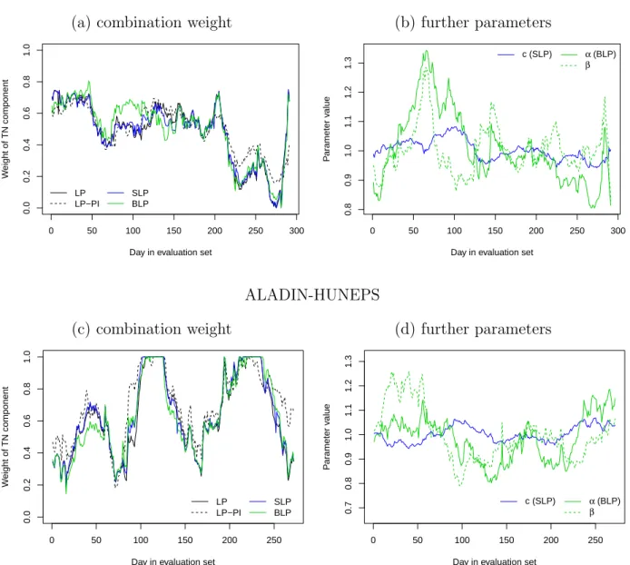
Figure 1: Illustration of mixture weights and other combination parameters for the LP, LP- PI, SLP and BLP combination methods over the corresponding verification periods for both wind speed data sets.

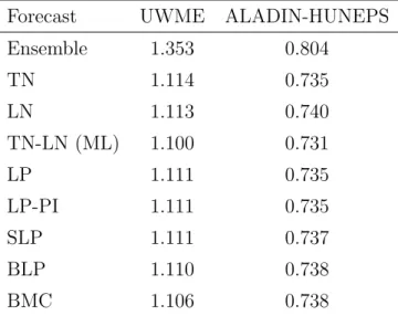
Table 1: Mean CRPS for probabilistic wind speed forecasts of the raw ensemble, the TN, LN and TN-LN (ML) EMOS models, and the forecast combination approaches.

Forecast UWME ALADIN-HUNEPS

Ensemble 1.353 0.804

TN 1.114 0.735

LN 1.113 0.740

TN-LN (ML) 1.100 0.731

LP 1.111 0.735

LP-PI 1.111 0.735

SLP 1.111 0.737

BLP 1.110 0.738

BMC 1.106 0.738

2007 were used to obtain training periods of equal length for all models which are validated on the data of calendar year 2008. For the ALADIN-HUNEPS data, the first 43 days are not included in the evaluation period (27 June 2012 – 31 March 2013) in order to compare all models over equal training periods.

Figure 1 graphically illustrates the resulting combination parameters for the LP, LP-PI, SLP and BLP methods. Here, the BMC method is excluded as the parameters vary over the random draws of the algorithm and do not allow for a straightforward summary. For both data sets, the estimated weight parameters are generally very similar for all methods, with minor deviations for the LP-PI and BLP approaches. The spread-adjustment parameter c in the SLP method does not vary much over time, whereas the α, β parameters in the BLP approach fluctuate much more rapidly.

Table 1 shows the mean CRPS values for all post-processing models and combination approaches for both data sets. All post-processing and combination methods substantially improve the raw ensemble forecasts. Among the post-processing models, the full TN-LN mixture model performs best, and the ranking of the TN and LN model depends on the data set at hand. For the UWME data, all forecast combination methods outperform the individual TN and LN component models, but are unable to compete with the TN-LN mixture model. The relative differences between the combination approaches are small, with the BLP and BMC approaches showing slightly better results. By contrast, none of the combination methods is able to perform better than the TN EMOS model for the ALADIN-HUNEPS data, and the SLP, BLP and BMC approaches result in slightly worse forecasts. Note that the BLP and SLP methods result in worse forecasts compared to the LP approach even though the latter arises as a special case for α = β = 1 and c = 1.

A potential explanation for these observations is the danger of over-fitting in choosing the optimal combination parameter values in the training sample that might not be optimal for the corresponding out of sample evaluation set. Further, the ALADIN-HUNEPS data set is comprised of only 10 observation stations. The training sets thus contain fewer forecast cases compared to the UWME data which might favor combination methods with a lower number of parameters.

To assess the variability of the observed score differences and the statistical significance of these findings, we utilize moving block bootstrap resampling (K¨unsch, 1989) and Diebold- Mariano (DM; Diebold and Mariano, 1995) tests described in the following. Both approaches allow to account for the temporal dependencies in the forecast errors. For a pair of forecast methods F₁, F₂, denote the vector of CRPS differences by (d₁, . . . , d_n), with

d_i(F₁, F₂) = CRPS(F₁⁽ⁱ⁾, x_i)−CRPS(F₂⁽ⁱ⁾, x_i),

where F_j⁽ⁱ⁾ denotes the forecast distribution F_j, j = 1,2, for forecast case i= 1, . . . , n in the evaluation set, and xi denotes the corresponding observation.

The moving block bootstrap resampling proceeds as follows: Randomly draw a starting date t∈ {1, . . . , T−b+ 1}, where T denotes the number of days in the evaluation set, and b is the block length. Then select all entries of (d1, . . . , dn) that correspond to any of the b consecutive days starting at t, i.e. select entries from all observation stations made at days t, t+ 1, . . . , t+b−1 and compute the mean value of this subset of (d₁, . . . , d_n). This procedure is repeated M times, and we subsequently assess the proportion of bootstrap resampling repetitions with negative mean score differences indicating a superior predictive performance of F₁.

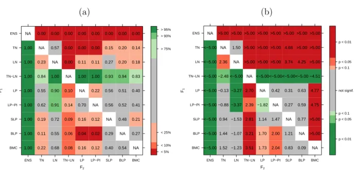
Figure 2(a) graphically summarizes the results of the block bootstrap resampling with a block length of b = 50 days, and M = 10 000 repetitions. Note that the size of the individual bootstrap samples thus differs for the two data sets due to the different number of observation stations. For the UWME data illustrated in the upper triangle, the differ- ences between the component models and the combination approaches are clearly visible and much more pronounced compared to the differences among the combination approaches where no clear trend can be detected. For the ALADIN-HUNEPS data (lower triangle), the combination methods exhibit some differences. In particular, the BLP approach per- forms considerably worse compared to the LP and LP-PI methods. For both data sets, the superiority of the full TN-LN mixture model forecasts is clearly visible.

DM tests are formal statistical tests of equal predictive performance based on the test statistic

t_n =√ n

d¯ ˆ σd

, where d¯ = ¹_nPn

i=1d_i and ˆσ_d is an estimator of the asymptotic variance of the score difference. Under standard regularity conditions, t_n is asymptotically standard normal under the null hypothesis of equal predictive performance of F₁ and F₂. Negative values

(a) (b)

F2

F1

BMC BLP SLP LP−PI LP TN−LN LN TN ENS

BMC BLP SLP LP−PI LP TN−LN LN TN ENS

1.00 0.22 0.68 0.08 0.16 0.12 0.40 0.54 NA 1.00 0.11 0.55 0.06 0.04 0.02 0.29 NA 0.27 1.00 0.19 0.72 0.09 0.16 0.12 NA 0.48 0.21 1.00 0.62 0.91 0.14 0.70 NA 0.56 0.52 0.41 1.00 0.55 0.90 0.10 NA 0.22 0.56 0.51 0.40 1.00 0.84 1.00 NA 1.00 1.00 0.93 0.94 0.83 1.00 0.23 NA 0.00 0.11 0.11 0.27 0.20 0.18 1.00 NA 0.57 0.00 0.00 0.00 0.15 0.20 0.14 NA 0.00 0.00 0.00 0.00 0.00 0.00 0.00 0.00

< 5%

< 10%

< 25%

> 75%

> 90%

> 95%

F2

F1

BMC BLP SLP LP−PI LP TN−LN LN TN ENS

BMC BLP SLP LP−PI LP TN−LN LN TN ENS

<−5.00 1.52 −1.23 3.51 1.73 2.04 0.83 0.09 NA

<−5.00 1.44 −1.07 3.21 1.70 2.00 1.21 NA >5.00

<−5.00 0.94 −1.53 2.81 1.14 1.47 NA 0.77 >5.00

<−5.00 −0.88 −3.37 2.39 −1.82 NA 0.27 0.59 4.75

<−5.00 −0.13 −3.27 2.70 NA 0.42 0.31 0.63 4.77

<−5.00 −2.48 <−5.00 NA <−5.00<−5.00<−5.00<−5.00 −4.51

<−5.00 2.36 NA >5.00 >5.00 >5.00 3.74 4.25 >5.00

<−5.00 NA 1.50 >5.00 >5.00 >5.00 4.68 >5.00 >5.00 NA >5.00 >5.00 >5.00 >5.00 >5.00 >5.00 >5.00 >5.00

p < 0.01 p < 0.05 p < 0.1 not signif.

p < 0.1 p < 0.05 p < 0.01

Figure 2: Summary of (a) block bootstrap resampling and (b) DM test results for both wind speed data sets and all pair-wise comparisons of forecasts. In both plots, the upper triangle contains results for the UWME data, and the lower triangle contains results for the ALADIN-HUNEPS data. In (a), the entry in row i and column j contains the proportion of bootstrap repetitions with negative mean score differences between F₁ and F₂, where F₁ is the forecast of the model in the i-th row, and F₂ is the forecast of the model in the j-th column, color-coded so that green (red) entries indicate superior performance of the model in the corresponding row (column). Similarly, values of the DM test statistic t_n are shown for comparisons of F₁ and F₂ in (b). The values of t_n are color-coded by the corresponding p-values of the test statistic under the null hypothesis of equal predictive performance.

of t_n indicate superior predictive performance of F₁, and F₂ is preferred if t_n is positive.

As an estimator ˆσ²_d , we use the sample autocovariance up to lag τ −1 in case of τ step ahead forecasts, see Baran and Lerch (2016) for details.

The corresponding results are summarized in Figure 2(b). Similar to the results of the block bootstrap resampling, the DM tests reveal a high level of significance of the score differences between the component models and the forecast combination approaches for the UWME data (upper triangle). By contrast, the score differences among the combination methods are not significant. Similar results can be observed for the ALADIN-HUNEPS data (lower triangle), where, however, the differences between the component and combined models are generally smaller and less significant. The only significant score differences among the combination methods are observed between BLP and the approaches based on the linear pool.

The improved predictive performance of the forecast combination approaches compared to the individual EMOS models based on single parametric distributions can be partially ex- plained by the improved calibration of the predictive distributions that will be demonstrated

UWME

Verification Rank

Relative Frequency

2 4 6 8

0.000.100.200.30

TN

PIT

Relative Frequency

0.0 0.2 0.4 0.6 0.8 1.0

0.00.51.01.52.02.53.0

LN

PIT

Relative Frequency

0.0 0.2 0.4 0.6 0.8 1.0

0.00.51.01.52.02.53.0

TN−LN

PIT

Relative Frequency

0.0 0.2 0.4 0.6 0.8 1.0

0.00.51.01.52.02.53.0

LP

PIT

Relative Frequency

0.0 0.2 0.4 0.6 0.8 1.0

0.00.51.01.52.02.53.0

LP−PI

PIT

Relative Frequency

0.0 0.2 0.4 0.6 0.8 1.0

0.00.51.01.52.02.53.0

SLP

PIT

Relative Frequency

0.0 0.2 0.4 0.6 0.8 1.0

0.00.51.01.52.02.53.0

BLP

PIT

Relative Frequency

0.0 0.2 0.4 0.6 0.8 1.0

0.00.51.01.52.02.53.0

BMC

PIT

Relative Frequency

0.0 0.2 0.4 0.6 0.8 1.0

0.00.51.01.52.02.53.0

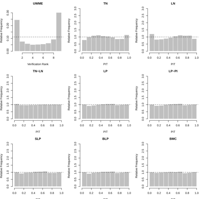
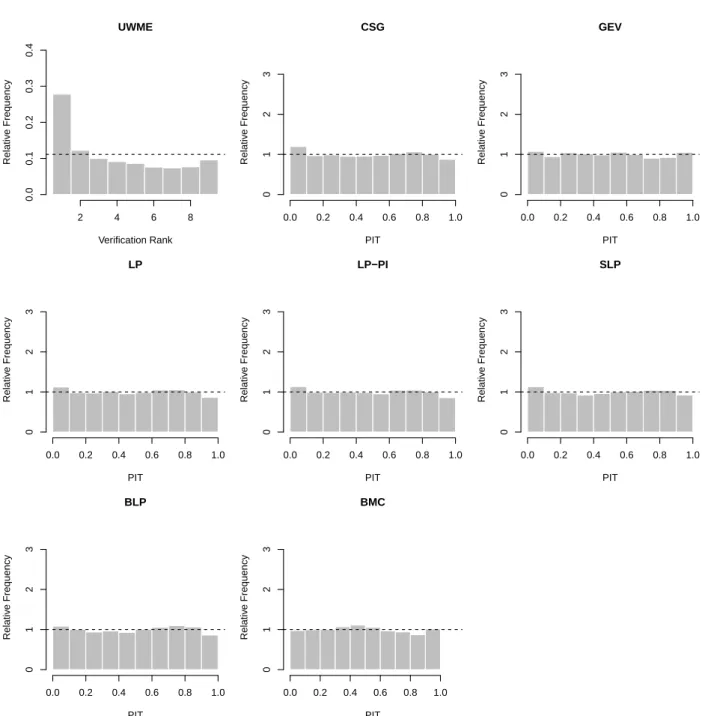
Figure 3: Verification rank histogram of raw ensemble forecasts and PIT histograms for post-processed and combined forecast distributions for the UWME data.

in the following. Calibration of the raw ensemble and the post-processed forecasts can be assessed graphically with the help of verification rank and probability integral transform (PIT) histograms, respectively. The former is the histogram of ranks of the validating ob- servations with respect to the corresponding ensemble predictions computed for all forecast cases (see e.g. Wilks, 2011, Section 7.7.2). For a calibrated ensemble, the observations and the ensemble forecasts should be exchangeable, resulting in a uniform verification rank his- togram. The PIT is the value of the predictive CDF evaluated at the verifying observation (Raftery et al., 2005), PIT histograms can therefore be seen as continuous counterparts of verification rank histograms. The visual inspection of deviations from the desired uniform distribution of the verification ranks and PIT values allows to further detect possible reasons of miscalibration (Gneiting et al., 2007).

A verification rank histogram of the raw ensemble forecast and PIT histograms of the post-processed and combined forecast distributions for the UWME data are shown in Fig- ure 3. Note that for the BMC forecasts PIT values are calculated for all 50 predictive CDFs of a given forecast case. Compared to the U-shaped verification rank histogram of the under- dispersive raw ensemble forecasts where the observation takes too many high and low ranks, all post-processing approaches are better calibrated which is indicated by smaller deviations from the desired uniform distribution of the PIT values. The calibration of the individual TN and LN component models is not perfect, with the TN model showing systematic over- predictions of high wind speeds, and the LN model over-predicting low wind speed values.

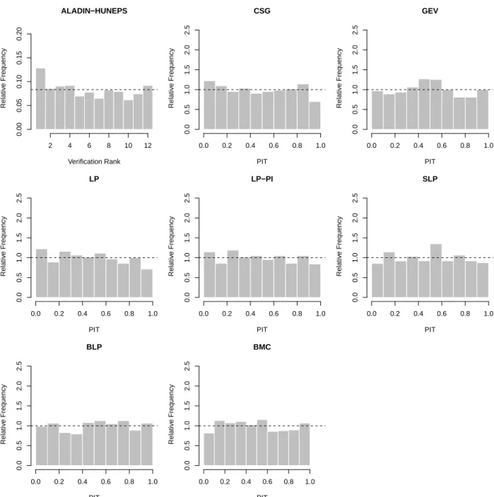
By contrast, all forecast combination approaches are able to correct for these deficiencies and are well calibrated, similar to the full TN-LN mixture model. The differences in cal- ibration among the combination methods are small, as the PIT histograms are virtually indistinguishable. The results for the ALADIN-HUNEPS data are qualitatively similar, the corresponding Figure 6 is shown in Appendix A.

5.2 Precipitation

Similar to wind speed, the post-processing models introduced in Section 3 are estimated using optimum score estimation approaches. The coefficients of the EMOS models (3.4) and (3.6) based on single CSG and GEV distributions are obtained using rolling training periods of lengths 70 (UWME) and 55 days (ALADIN-HUNEPS), which ensures comparability with Baran and Nemoda (2016).

Given the estimated coefficients of the CSG and GEV component models, the parameters of the two-step combination approaches are estimated as described for wind speed. For the UWME data, forecast cases from calendar year 2007 are again used to obtain training periods of equal length for all models, whereas the first 55 days are excluded from the evaluation period of the ALADIN-HUNEPS data. In this way UWME forecasts are again validated on data from calendar year 2008, whereas the verification period for ALADIN-HUNEPS precipitation forecasts is 21 January – 25 March 2011.

UWME

(a) combination weight (b) further parameters

0 50 100 150 200 250 300

0.00.20.40.60.81.0

Day in evaluation set

Weight of CSG component

LP LP−PI

SLP BLP

0 50 100 150 200 250 300

0.81.01.21.41.6

Day in evaluation set

Parameter value

c (SLP) α (BLP) β

ALADIN-HUNEPS

(c) combination weight (d) further parameters

0 10 20 30 40 50 60

0.00.20.40.60.81.0

Day in evaluation set

Weight of CSG component

LP LP−PI

SLP BLP

0 10 20 30 40 50 60

0.60.70.80.91.01.11.21.3

Day in evaluation set

Parameter value

c (SLP) α (BLP) β

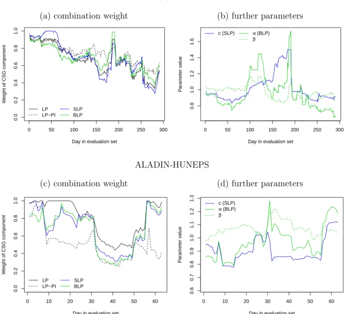
Figure 4: Illustration of mixture weights and other combination parameters for the LP, LP- PI, SLP and BLP combination methods over the corresponding verification periods for both precipitation data sets.

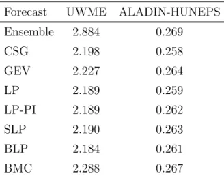
Table 2: Mean CRPS for probabilistic precipitation accumulation forecasts of the raw en- semble, the CSG and GEV EMOS models, and the forecast combination approaches.

Forecast UWME ALADIN-HUNEPS

Ensemble 2.884 0.269

CSG 2.198 0.258

GEV 2.227 0.264

LP 2.189 0.259

LP-PI 2.189 0.262

SLP 2.190 0.263

BLP 2.184 0.261

BMC 2.288 0.267

The estimates of the combination parameters over the evaluation period are shown in Figure 4. The mixture weights of the LP, LP-PI, SLP and BLP approaches exhibit relatively similar developments over time, and the spread-adjustment parameter c shows slightly higher variability compared to the wind speed forecasts.

Mean CRPS values for all post-processing models and forecast combination methods for both data sets are shown in Table 2. Compared to wind speed, the relative improvements of both EMOS models over the raw ensemble forecasts are smaller, particularly for the ALADIN-HUNEPS data. This observation is in line with various comparative studies of post-processing models for different variables (see for example Hemri et al., 2014). The CSG model outperforms the GEV model, and in case of the UWME data, the predictive performance is further improved by combining the forecasts via the LP, LP-PI, SLP and BLP approaches which show small relative differences. In light of the larger relative score differences in favor of the CSG method it is worth noting that the estimated mixture weights of the CSG component in these combination approaches are between 0.3 and 0.7 for a large number of forecast cases, see Figure 4. As observed for wind speed, none of the combination methods is able to outperform the best component model for the ALADIN-HUNEPS data.

Forecasts produced by the BMC method are worse than both component models for both data sets and only marginally better than the raw ensemble forecasts in case of the ALADIN- HUNEPS data.

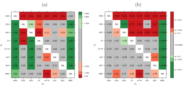
The variability and statistical significance of the observed score differences is again as- sessed using moving block bootstrap resampling and DM tests with the setup described above. The results are summarized in Figure 5. For the ALADIN-HUNEPS data, the block bootstrap resampling indicates clear differences between the raw ensemble forecasts and all post-processing and forecast combination approaches. Further, the GEV model forecasts are substantially improved by the LP, LP-PI, SLP and BLP combination methods. These