for calibrating the wind speed forecasts in central regions of Chile ∗

(1)

Post-processing methods

for calibrating the wind speed forecasts in central regions of Chile ^∗

Mailiu Díaz

^ab

, Orietta Nicolis

^bc

, Julio César Marín

^ac

, Sándor Baran

^d

aDepartamento de Meteorología, Universidad de Valparaíso, Chile mailiudp@gmail.com

bFacultad de Ingenieria, Universidad Andres Bello, Chile orietta.nicolis@unab.cl

cCentro Interdisciplinario de Estudios Atmosfŕicos y Astro-Estadística, Universidad de Valparaíso, Chile

julio.marin@meteo.uv.cl

dFaculty of Informatics, University of Debrecen, Hungary baran.sandor@inf.unideb.hu

Submitted: December 22, 2020 Accepted: March 17, 2021 Published online: May 18, 2021

Abstract

In this paper we propose some parametric and non-parametric post-processing methods for calibrating wind speed forecasts of nine Weather Research and Forecasting (WRF) models for locations around the cities of Valparaíso and Santiago de Chile (Chile). The WRF outputs are generated with different planetary boundary layers and land-surface model parametrizations and they are calibrated using observations from 37 monitoring stations. Statistical calibration is performed with the help of ensemble model output statistics and quantile regression forest (QRF) methods both with regional and semi-local approaches. The best performance is obtained by the QRF using a semi- local approach and considering some specific weather variables from WRF simulations.

∗This research was partially supported by the Interdisciplinary Center of Atmospheric and Astro-Statistical Studies, University of Valparaíso, Chile.

doi: https://doi.org/10.33039/ami.2021.03.012 url: https://ami.uni-eszterhazy.hu

93

(2)

Keywords:Ensemble model output statistics, ensemble calibration, quantile regression forest, statistical post-processing, wind speed

1. Introduction

Numerical weather prediction (NWP) models have been used for many years in research and operational weather forecasting due to their advantage to simulate the state of the atmosphere in any region of the globe at high spatial and tem- poral resolutions. The Weather Research and Forecasting (WRF) model [32, 37]

is one of the most widely used systems, which has received strong support by the atmospheric science community over the years. However, despite its continuous improvement and successful use, the model still presents biases in the prediction of near-surface variables; specifically, in the prediction of wind speed over complex terrain [23, 33, 35], which may be related to the smoothed topography used in the model and the misrepresentation of small-scale atmospheric processes [19, 23]. Those limitations negatively influence obtaining accurate predictions of surface wind speed and direction, which are used in a large number of applications in Chile, such as wind energy [24, 28], air-quality [6, 33, 36], and precipitation over the Andes cordillera [9].

In the last 15 years several statistical post-processing models have been devel- oped to obtain sharp and calibrated forecasts, e.g. the non-homogeneous regression or ensemble model output statistics [EMOS; 13], which method provides full predictive distribution of the future weather quantity using a single parametric distribution with parameters connected to the ensemble members.

Recently, some studies have been focused on the use of machine learning techniques for statistical post-processing. [39] introduced a new post-processing method based on quantile regression forests (QRF), which is a generalization of random forests and allows the estimation of conditional quantiles from the cumulative distribution function (CDF) in an efficient and simple way. This approach has the important advantage of allowing the inclusion of other features as predictors in the post-processing model. One can also mention [34], where QRF is applied to improve 2m temperature forecasts and a flexible alternative using a neural network is also proposed.

In [7], we evaluated two parametric models for calibrating surface temperature forecasts from nine WRF simulations at 19 meteorological stations in Santiago city.

Now, the main aim of this study is to compare the forecast skill of some parametric and non-parametric post-processing methods to calibrate the wind speed using both regional and semi-local approaches at 37 monitoring stations around Valparaíso and Santiago city. Furthermore, the importance of each simulation and that of other weather variables from WRF included as predictors in QRF are examined on the basis of the continuous ranked probability score (CRPS).

The paper is organized as follows. Section 2 provides a description of data from meteorological stations, WRF configurations and variables included in the study, and a preliminary statistical analysis considering the error forecast and verification

(3)

rank. Methods for modeling wind speed and some verification tools are described in Section 3. The results of statistical post-processing are given in Section 4 with a comparison of the various approaches and with specification of the importance of ensemble members and other included variables. Finally, Section 5 presents the major results and some possible future extensions.

2. Description of the data and preliminary analysis

Nine WRF simulations were generated for the period between 1 June 2017 and 30 January 2018 to predict wind speed at 37 meteorological stations, around Val- paraíso and Santiago cities, using the same configurations of [7]. The WRF simulations and the data from monitoring stations are briefly described below. A preliminary analysis of the forecasts is also provided.

2.1. WRF configurations and data description

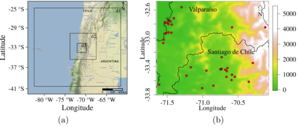
The Advanced Research WRF core (ARW-WRF) [37] Version 3.7.1 was employed to generate a nine-member forecast ensemble using three nested domains at 18 km, 6 km and 2 km horizontal resolutions (see Figure 1a) and 44 vertical levels with variable resolution between 60 and 200 m from 1 June 2017 to 30 January 2018 at 3 hour time steps from 00 UTC to 21 UTC. The detailed description of nine ensemble members is presented in [7].

(a) (b)

Figure 1. (a) Representation of the domains 1, 2 and 3 used in the WRF model at 18 km, 6 km, and 2 km horizontal resolutions respectively and (b) Altitude map and the location of monitoring

stations represented with red points.

The ensemble members differ both in the applied planetary boundary layer (PBL) and land-surface model (LSM) parametrizations. The Land-surface processes are represented by the 5-layer [8], Noah [5] and Pleim-Xiu [31] schemes;

we use the Mellor-Yamada-Janjic (MYJ) [18], Yonsei University (YSU) [16] and

(4)

Mellor-Yamada Nakanishi and Ninno 2.5 level (MYNN) [29] schemes to represent the PBL and surface layer processes.

The rest of the parametrizations are kept the same in all simulations: Kain- Fritsch (Kain-F) [20] cumulus parametrization, the Rapid Radiative Transfer Model (RRTMG) [17] to represent the long wave and short wave radiative processes, and the WRF single-moment 3-class (WSM3) [15] scheme to represent microphysics processes.

The initial and boundary conditions were provided by the Final Operational Global Analysis (FNL) at 0.25 ×0.25 degrees horizontal resolution every 6 hours to obtain the variables described in Table 1 from the highest resolution domain (d3).

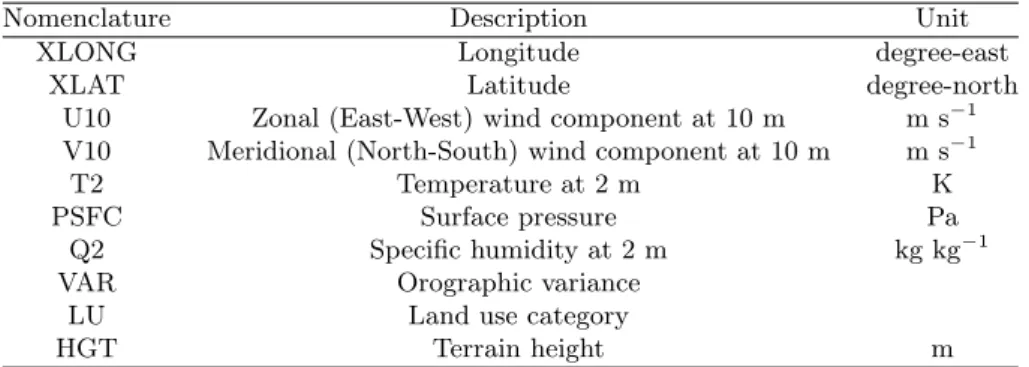
Table 1. The variables included in the study from the highest resolution domain (d3) of WRF simulations.

Nomenclature Description Unit

XLONG Longitude degree-east

XLAT Latitude degree-north

U10 Zonal (East-West) wind component at 10 m m s⁻¹ V10 Meridional (North-South) wind component at 10 m m s⁻¹

T2 Temperature at 2 m K

PSFC Surface pressure Pa

Q2 Specific humidity at 2 m kg kg⁻¹

VAR Orographic variance

LU Land use category

HGT Terrain height m

Wind speed and relative humidity forecasts are obtained from the predictions of variables described in Table 1: 10 m wind speed equals WS =√

U10²+V10² and it is expressed in m s⁻¹, whereas 2 m relative humidity is obtained using an approximation of equations presented by [3], namely

RH=Q2/(︀

(𝑝𝑞0/PSFC) exp{𝑎2(T2−𝑎3)/(T2−𝑎4)})︀

, (2.1)

where 𝑝𝑞0= 379.91, 𝑎2 = 17.27,𝑎3= 273.16and 𝑎4= 35.86. The values obtained by equation (2.1) are normed to 1 and referred to as percents.

Finally, the corresponding 3 hourly verifying observations of 10 m wind speed for the same time period 1 June 2017 - 30 January 2018 measured in 37 monitoring stations around Valparaíso and Santiago city (see Figure 1b) were downloaded from the Dirección Meteorológica de Chile (http://www.meteochile.gob) and the National System for Air Quality (https://sinca.mma.gob.cl/). The stations have different altitudes represented in meters from 0 to 3000 m, see Figure 1 (b).

2.2. Preliminary data analysis

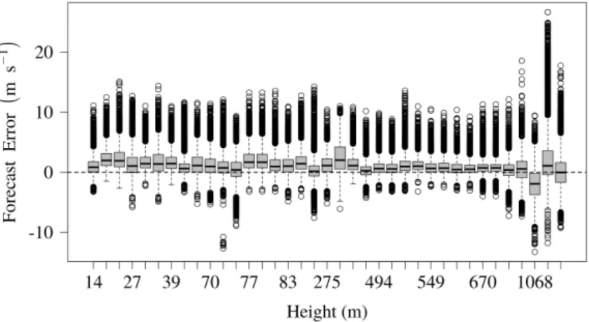
Consider first the dependence of the forecast error of an individual member of the WRF ensemble forecast on the location of the monitoring station. In Figure 2 the

(5)

box-plots of forecast errors corresponding to different stations are given, arranged in ascending order of station altitude. The median error at all stations is close to 0; however, as expected, stations above 2000 m located in the mountain zone of Santiago de Chile exhibit the highest forecast errors (last two boxplots in Figure 2), which is nicely in line with the results of [25].

Figure 2. Forecast error at each station sorted by the altitude in meters.

(a) (b)

Figure 3. (a) Verification rank histogram for the total period and (b) the percentage of observed values included in the range of the

ensemble forecasts at each hour for the all period.

Further, to get an idea about the calibration, Figures 3a,b show the verification rank histogram of raw wind speed ensemble forecasts and the coverage for the different observation times, respectively. The verification rank is the rank of the validating observation with respect to the corresponding ensemble members and in

(6)

the case of proper calibration it should be uniformly distributed (see e.g. Section 9.7.1 [42]), whereas the coverage is the proportion of observed values included in the range of the forecasts. Since, the resulted histogram doesn’t follow a uniform distribution as confirmed by the high value of the𝜒²test statistic, a great difference between the observed and the expected frequencies is supposed to exist. In addition, there is no observation hour when the coverage exceeds 50% with the lowest value of 41.99% at 21 UTC (see Figure 3b), which proportions are far from the nominal 80% coverage of a calibrated 9-member ensemble forecast.

These preliminary results indicate that the ensemble forecasts are biased and not properly calibrated calling for some form of statistical post-processing.

3. Methodology

As wind speed data are characterized by non-negative values and the observations do not follow a symmetric law, they cannot be described by a normal distribution as temperature or air pressure. For this reason, to model wind speed the use of skewed and non-negative distributions, such as a truncated normal [1, 41], log-normal [2]

or gamma [38] distribution are proposed.

Some post-processing approaches to calibrate wind speed forecasts and the tools to assess the forecast skill of the models are described below.

3.1. EMOS using truncated normal distribution

The Ensemble Model Output Statistics (EMOS) or non-homogeneous regression approach, proposed by [13], is one of the most used parametric post-processing techniques. EMOS models for various weather variables differ in the predictive distribution family and in the link functions connecting the parameters of the predictive distribution to the ensemble members. Following [41], as parametric family we consider a truncated normal (TN) distribution𝒩⁰(𝜇, 𝜎)with location𝜇, scale𝜎 >0 and cut-off equal at0, defined by probability density function (PDF)

𝑓(𝑥|𝜇, 𝜎) :=

{︃₁

𝜎𝜑((𝑥−𝜇)/𝜎)/Φ(𝜇/𝜎), if𝑥≥0,

0, otherwise, (3.1)

[41], where𝜑andΦare the PDF and the cumulative distribution function (CDF) of a standard normal distribution, respectively.

The TN EMOS predictive distribution considering 9 WRF ensemble members is defined as

𝒩⁰(𝑎0+𝑎1𝑓1+· · ·+𝑎9𝑓9, 𝑏0+𝑏1𝑆²), where 𝑆²:= 1 8

∑︁9

𝑘=1

(𝑓𝑘−𝑓¯)², with 𝑓¯ denoting the ensemble mean. Location parameters 𝑎0, 𝑎1, . . . , 𝑎9 ∈ R, 𝑎1, . . . , 𝑎9≥0 and scale parameters0≤𝑏0, 𝑏1∈Rare estimated over the training

(7)

data consisting of ensemble members and verifying observations from the preceding 𝑛days (rolling training period) by optimizing the mean of a certain proper verification score (see [41] for more details), which in our case is the continuous ranked probability score (CRPS) described in detail in Section 3.2.

3.2. Diagnostics

[11] defines the aim of statistical post-processing as maximization of the sharpness of the predictive distribution subject to calibration, where the latter expresses a statistical consistency between forecasts and observations, whereas the former indicates the forecast accuracy.

For doing a simultaneous evaluation of calibration and sharpness, [12] suggests the use of the continuous ranked probability score (CRPS), which for a given CDF 𝐹(𝑦)and observation𝑥is defined as

CRPS(𝐹, 𝑥) :=

∫︁∞

−∞

(︀𝐹(𝑦)−1_{𝑦≥𝑥}

)︀2

d𝑦=E|𝑋−𝑥| −1

2E|𝑋−𝑋^′|,

where 1_{𝑦≥𝑥} denotes the indicator function which is 1 if𝑦 ≥𝑥and 0 otherwise, while 𝑋 and 𝑋^′ are independent random variables with CDF 𝐹 and finite first moment. For wind speed, similar to observations and forecasts, this score is expressed in m s⁻¹and it is a negatively oriented scoring rule, that is the smaller the better. For comparing predictive performance of different probabilistic forecasts one usually considers the mean CRPS over all forecasts and observations of the verification data denoted byCRPS.

In addition, to assess the relative improvement of a forecast with respect to a given reference forecast, one can calculate the continuous ranked probability skill score (CRPS.S) [12],

CRPS.S = 1− CRPS CRPSref,

whereCRPSrefdenotes the mean CRPS of the reference forecast over the verification data.

Further, calibration can also be investigated by examining the coverage of the (1−𝛼)100% central prediction interval with 𝛼 ∈ (0,1), i.e. by calculating the proportion of validating observations located between the lower and upper 𝛼/2 quantiles of the predictive distribution. In the case of proper calibration the coverage should be around(1−𝛼)100%, and in order to provide a fair comparison with the raw ensemble one usually chooses the value of𝛼to match the nominal coverage of the raw ensemble (80 %for the 9-member ensemble).

The predictive performance of point forecasts can be assessed by considering the root mean of the squared error 𝑆𝐸(𝑥, 𝑦) = (𝑥−𝑦)² (RMSE) and mean of the absolute error 𝐴𝐸(𝑥, 𝑦) = |𝑥−𝑦| (MAE) based on the forecast 𝑦 and the observation 𝑥[10, 30] taken over all forecast cases in the verification data.

(8)

Finally, the probability integral transform (PIT) histograms (see e.g. [42]) might be used for a visual perception of the improvement in calibration compared with the raw ensemble. The PIT is the value of the predictive CDF evaluated at the validating observation and for a calibrated forecast PIT has to follow a uniform law on the[0,1]interval. Hence, the PIT histogram is the continuous counterpart of the verification rank histogram of the raw ensemble.

3.3. Quantile Regression Forests

As an alternative to parametric post-processing, [39] and [34] recently applied the Quantile Regression Forest (QRF) model for calibrating ensemble forecasts. This model was originally introduced by [26] as an extension of the random forest theory [4], by presenting an algorithm for computing the estimated distribution of the variable of interest, in our case the wind speed. The algorithm consists of an iterative process which splits the training data and every split minimizes the sum of the variance of the response variable. One of the disadvantages of this method is that the process of growing trees might lead to overfitting as mentioned in [22].

However, [39] suggested to solve this problem by tuning the number of trees.

Different predictors can be used in the implementation of the QRF (see for example [39] and [34]); here we consider two cases. For the first one the only predictors are the nine wind speed forecasts from the WRF model. In the second case this set is extended by the mean, standard deviation, minimum and maximum of some variables presented in Table 1 (U10, V10, T2, PSFC, and RH) in addition to the orographic variance (VAR), land use (LU), HGT, and the observed altitude (Alt_st), forming a total of 24 covariates. In particular, our implementation is based on theRpackagequantregForest.

The QRF model also allows to determine the importance of the predictor𝑝𝑗 by the random permutation method introduced in the context of random forests by [4]. The importance is computed by the mean CRPS of the difference between the forecast𝐹 conditional to the permuted predictor and the unpermuted features, i.e.

Imp(𝑝𝑗) = 1 𝑆𝑇

∑︁𝑆

𝑠=1

∑︁𝑇

𝑡=1

(︀CRPS(𝐹 |𝑋_𝑠,𝑡^𝑝^𝑗, 𝑦𝑠,𝑡)−CRPS(𝐹 |𝑋𝑠,𝑡, 𝑦𝑠,𝑡))︀

, (3.2)

where𝑋_𝑠,𝑡^𝑝^𝑗 denotes the vector of predictors at time𝑡and station𝑠for the permuted predictor (see [34] for more details). The higher the value of Imp(𝑝𝑗), the more important the predictor𝑝𝑗.

3.4. Spatial selection of training data

For selecting the geographical composition of the training data for post-processing methods, [41] defines the local and regional approaches. By regional or global we mean that forecast/observation pairs of all stations from the training period are used to estimate the parameters of a given parametric model or perform a non- parametric calibration, while the local approach uses only the information of the

(9)

observation site at hand. Although the local approach in general results in better predictive performance, it requires longer training periods to avoid numerical sta- bility issues [21]. Hence, we focus on regional estimation and on the novel semi-local approach proposed by [21]. Semi-local modeling takes the advantages of regional and local forecasting by clustering the observation stations based on climatological characteristics and the distribution of forecast errors of the training data and performing a global estimation within each cluster. Clustering is performed with the help of a𝑘-means algorithm [14] and clusters may vary as the training window slides.

4. Results

In order to exclude the effect of natural daily variation in wind speed, calibration approaches described in Sections 3.1 and 3.3 were run separately for each forecast hour using an optimal training period length and both regional and semi-local approaches.

4.1. Selection of the training data

Selection of an appropriate set of training data is necessary for successful calibration. This selection procedure includes the choice of the length of the rolling training period and the geographical composition of the training set.

The optimal length of the training period is obtained by verifying the forecasts against observations for different training periods with the help of various scoring rules [12]. We investigated the mean CRPS and nominal coverage of the regional EMOS predictive distribution for the time period from 29 September 2017 to 30 January 2018 separately at each forecast hour using training periods of length 55, 60, 65, . . . , 120days. Based on the corresponding figures of the mean CRPS and nominal coverage plotted against the training period length (not shown) we decided to choose a training period of length 65 days for calibrating wind speed forecasts of the WRF simulations. This length of the training period leaves 179 calendar days between 5 August 2017 and 30 January 2018 for forecast verification.

As mentioned in Section 3.4, EMOS and QRF modeling were performed using regional and clustering-based semi-local training. In the latter approach stations were grouped into 3 clusters using 24 features, where half of the features were obtained as equidistant quantiles of the climatological CDF, whereas the other half as equidistant quantiles of the empirical CDF of the forecast error over the training period [21]. Note that each verification day and forecast hour had an individual clustering of the 37 monitoring stations.

4.2. Comparison of the post-processed forecasts

EMOS and QRF calibration of WRF ensemble forecasts is performed using the optimal 65 day rolling training period and regional and semi-local approaches to

(10)

spatial selection of training data. In what follows EMOS_C and QRF_C will denote the semi-local EMOS and QRF methods, respectively, in order to distinguish them from the corresponding regional approaches. Note that EMOS model (3.1) has 12 parameters to be estimated from the training data.

Further, as mentioned is Section 3.3, QRF method is implemented in two different ways. In the first case, referred to as QRF, we use just the nine wind speed forecasts from the WRF model, whereas in the second case (QRF_M), this set is extended by several other variables (see Section 3.3) resulting in a total of 24 covariates. Both cases were tested with different arguments and we decided to make use of the model with 300 trees and a minimum size of 5 for terminal leaves, since these arguments provided smaller scores. Further, the implementations of QRF and QRF_M differ from each other in the number of variables randomly sampled as candidates at each split; one for QRF and three for QRF_M were the best options.

Figure 4. Mean CRPS vs. EMOS by hours for all stations.

Consider first Figure 4 showing the CRPS.S values with respect to the regional EMOS approach as function of the forecast hour. The use of semi-local estimation in EMOS modeling improves the calibration at each hour and the same applies for QRF modeling. QRF models perform slightly better than the corresponding EMOS approaches and the best QRF forecasts are obtained by adding other features as predictors to the regression model (QRF_M and QRF_C_M). Although the (QRF_M and QRF_C_M) provided better predictions than all the other methods (see Figure 4), the results could be further improved buy adding new covariates, for example using the wind speed forecasts instead of the U10 and V10 components.

Note that the ranking of the different methods is completely consistent, the different graphs do not cross.

(11)

Table 2. Overall scores for the different models computed in the study.

Models CRPS MAE RMSE Coverage

Ensemble 1.1715 1.4470 1.9949 43.95

EMOS 0.6078 0.8333 1.2443 82.12

EMOS_C 0.5108 0.7121 1.0361 80.29

QRF 0.5794 0.7968 1.1827 89.15

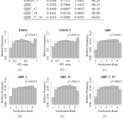
QRF_C 0.4939 0.6867 0.9817 88.18 QRF_M 0.4441 0.6143 0.9021 90.69 QRF_C_M 0.4318 0.5992 0.8781 89.65

(a) (b) (c)

(d) (e) (f)

Figure 5. PIT histograms of post-processed forecasts (a) EMOS and (b) EMOS-C, and verification rank histogram of: (c) QRF, (d)

QRF-C, (e) QRF-M, (f) QRF-C-M.

A similar ranking of the post-processing methods can be derived from the overall scores of Table 2. All post-processing approaches outperform the raw WRF ensemble in all scores with a wide margin, and the lowest CRPS, MAE and RMSE belong to QRF_M and QRF_C_M combined with slightly high coverage values.

Finally, as mentioned in Section 3.2, PIT and verification rank histograms allow us to visualize the improvement in calibration, and the goodness of fit to the cor-

(12)

responding uniform distribution can be quantified by the value of the 𝜒² statistic (the smaller the better). According to Figure 5, all post-processing methods can successfully correct the underdispersion of the raw WRF ensemble forecast (see Figure 3a) turning it into a slight overdispersion indicated by the hump shape of the histograms. However, none of PIT histograms looks close to uniformity, prob- ably due to the small sample size [40]. EMOS forecast are slightly biased and from the competing QRF approaches QRF-C seems to have the best calibration with 𝜒²= 1647.9.

4.3. Importance features results

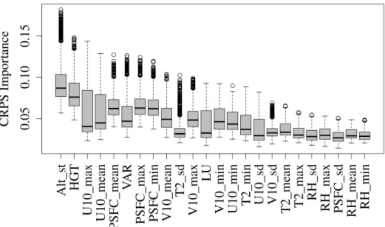
Additionally to the comparison of the post-processing methods, the QRF model allows to determine the importance of each predictor by considering the CRPS as verification score using equation (3.2). Figure 6 shows that the observed altitude (Alt-st) and the terrain height from WRF model are the most important variables in the QRF-M. The zonal near-surface wind component (U10) seems to be more important than the meridional wind component (V10), and the surface pressure (PSFC), orographic variance (VAR) and the deviation of surface temperature (T2) are also included in the first ten most important features.

Figure 6. Importance of the forecasts considering the CRPS score.

5. Conclusions

In this work some parametric and non-parametric post-processing methods for calibrating 9-member 3 hourly WRF wind speed ensemble forecasts are investigated.

The WRF ensemble forecasts were generated by different planetary boundary layers and land-surface model parametrizations in order to model wind speed at 37 monitoring stations around Valparaíso and Santiago city for the period between 1 June 2017 and 30 January 2018. In order to choose the optimal training pe-

(13)

riod length (65 days in this study) a regional EMOS model has been tested with training periods of different lengths. EMOS and QRF modeling is performed both regionally and using a clustering-based semi-local approach, the different forecast hours are treated separately in order to exclude the natural daily variation in wind speed.

Compared with raw WRF ensemble forecasts, all post-processing approaches result in a substantial improvement in calibration of probabilistic and accuracy of point forecasts. From the competing approaches to calibration, the semi-local QRF model considering other weather variables from WRF simulations exhibits the best overall predictive performance.

The importance of the predictors for QRF using a permutation method is also investigated, where from the additional covariates the altitude of the station occurs to be the most important. These results are crucial in choosing the parametrization for the WRF model in order to improve wind predictions in Chile.

As a next step we are planning to explore other machine learning methods in addition to different parametrizations. Further, it would be very interesting to evaluate the performance of EMOS models with additional predictors using the boosting approach proposed by [27].

Acknowledgments. Mailiu Díaz is grateful for the support of the National Com- mission for Scientific and Technological Research (CONICYT) of Chile under Grant No. 21150227. Orietta Nicolis and Julio César Marín are partially supported by the Interdisciplinary Center of Atmospheric and Astro-Statistical Studies. Pow- ered@NLHPC: This research was partially supported by the supercomputing in- frastructure of the National Laboratory for High Performing Computer (NLHPC) (ECM-02). Sándor Baran was supported by the National Research, Development and Innovation Office under Grant No. NN125679.

References

[1] S. Baran:Probabilistic wind speed forecasting using Bayesian model averaging with truncated normal components, Computational Statistics and Data Analysis 75 (2014), pp. 227–

238,

doi:https://doi.org/10.1016/j.csda.2014.02.013.

[2] S. Baran,S. Lerch:Log-normal distribution based EMOS models for probabilistic wind speed forecasting, Quarterly Journal of the Royal Meteorological Society 141 (2015), pp. 2289–

2299,

doi:https://doi.org/10.1002/qj.2521.

[3] D. Bolton:The computation of equivalent potential temperature, Monthly Weather Review 108 (1980), pp. 1046–1053,

doi:https://doi.org/10.1175/1520-0493(1980)108<1046:TCOEPT>2.0.CO;2.

[4] L. Breiman:Random Forests, Machine Learning 45.1 (2001), pp. 5–32,issn: 1573-0565, doi:https://doi.org/10.1023/A:1010933404324.

(14)

[5] F. Chen,J. Dudhia:Coupling an Advanced Land Surface-Hydrology Model with the Penn State-NCAR MM5 Modeling System. Part I: Model Implementation and Sensitivity, Monthly Weather Review 129.4 (2001), pp. 569–585,

doi:https://doi.org/10.1175/1520-0493(2001)129<0569:CAALSH>2.0.CO;2.

[6] A. M. Córdova,J. Arévalo,J. C. Marín,D. Baumgardner,G. B. Raga,D. Pozo, C. A. Ochoa,R. Rondanelli:On the transport of urban pollution in an Andean mountain valley, Aerosol & Air Quality Research 16 (2016), pp. 593–605,

doi:https://doi.org/10.4209/aaqr.2015.05.0371.

[7] M. Díaz,O. Nicolis,J. Marín,S. Barán:Statistical post-processing of ensemble forecasts of temperature in Santiago de Chile, Meteorological Applications 27.1 (2019),

doi:https://doi.org/10.1002/met.1818.

[8] J. Dudhia:A Multi-layer Soil Temperature Model for MM5. The Sixth PSU/NCAR Meso- scale Model Users’ Workshop, in: July 1996.

[9] Y.-M. G.,J. Gironás,M. Caneo,R. Delgado,R. Garreaud:Using the Weather Re- search and Forecasting (WRF) Model for Precipitation Forecasting in an Andean Region with Complex Topography, Atmosphere 9.8 (2018), p. 304,

doi:https://doi.org/10.3390/atmos9080304.

[10] T. Gneiting:Making and evaluating point forecasts, Journal of the American Statistical Association 106.494 (2011), pp. 746–762.

[11] T. Gneiting, F. Balabdaoui,A. E. Raftery:Probabilistic forecasts, calibration and sharpness, Journal of the Royal Statistical Society: Series B 69 (2007), pp. 243–268.

[12] T. Gneiting,A. E. Raftery: Strictly proper scoring rules, prediction, and estimation, Journal of the American Statistical Association 102.477 (2007), pp. 359–378,

doi:https://doi.org/10.1198/016214506000001437.

[13] T. Gneiting, A. E. Raftery,A. H. Westveld,T. Goldman: Calibrated Probabilis- tic Forecasting Using Ensemble Model Output Statistics and Minimum CRPS Estimation, Monthly Weather Review 133.5 (2005), pp. 1098–1118,

doi:https://doi.org/10.1175/MWR2904.1.

[14] J. A. Hartigan,M. A. Wong:Algorithm AS 136: A K-means clustering algorithm, Ap- plied Statistics 28 (1979), pp. 100–108,

doi:https://doi.org/10.2307/2346830.

[15] S.-Y. Hong,J. Dudhia,S.-H. Chen:A Revised Approach to Ice Microphysical Processes for the Bulk Parameterization of Clouds and Precipitation, Monthly Weather Review 132.1 (2004), pp. 103–120,

doi:https://doi.org/10.1175/1520-0493(2004)132<0103:ARATIM>2.0.CO;2.

[16] S.-Y. Hong,Y. Noh,J. Dudhia: A New Vertical Diffusion Package with an Explicit Treatment of Entrainment Processes, Monthly Weather Review 134.9 (2006), pp. 2318–2341, doi:https://doi.org/10.1175/MWR3199.1.

[17] M. J. Iacono, J. S. Delamere, E. J. Mlawer, M. W. Shephard, S. A. Clough, W. D. Collin:Radiative forcing by long-lived greenhouse gases: Calculations with the AER radiative transfer models, Journal of Geophysical Research: Atmospheres 113.D13 (2008), doi:https://doi.org/10.1029/2008JD009944.

[18] Z. I. Janjić:The Step-Mountain Eta Coordinate Model: Further Developments of the Con- vection, Viscous Sublayer, and Turbulence Closure Schemes, Monthly Weather Review 122.5 (1994), pp. 927–945,

doi:https://doi.org/10.1175/1520-0493(1994)122<0927:TSMECM>2.0.CO;2.

[19] P. A. Jiménez,J. Dudhia:Improving the Representation of Resolved and Unresolved To- pographic Effects on Surface Wind in the WRF Model, Journal of Applied Meteorology and Climatology 51 (2012), pp. 300–316,

doi:https://doi.org/10.1175/JAMC-D-11-084.1.

(15)

[20] J. S. Kain:The Kain-Fritsch Convective Parameterization: An Update, Journal of Applied Meteorology 43.1 (2004), pp. 170–181,

doi:https://doi.org/10.1175/1520-0450(2004)043<0170:TKCPAU>2.0.CO;2.

[21] S. Lerch,S. Baran:Similarity-based semi-local estimation of EMOS models, Journal of the Royal Statistical Society: Series C 66 (2017), pp. 29–51.

[22] Y. Lin,Y. Jeon:Random Forests and Adaptive Nearest Neighbors, Journal of the American Statistical Association 101 (2006), pp. 578–590.

[23] J. C. Marí n,D. Pozo,E. Mlawer,D. Turner,M. Curé:Dynamics of local circulations in mountainous terrain during the RHUBC-II project, Monthly Weather Review 141.10 (2013), pp. 3641–3656,

doi:https://doi.org/10.1175/MWR-D-12-00245.1.

[24] C. Mattar,D. Borvarán:Offshore wind power simulation by using WRF in the central coast of Chile, Renewable Energy 94 (2016), pp. 22–31,

doi:https://doi.org/10.1016/j.renene.2016.03.005.

[25] A. Mazzeo,N. Huneeus,C. Ordóñez,A. Orfanoz-Cheuquelaf,L. Menut,S. Mail- ler,M. Valari,H. Denier van der Gon,L. Gallardo,R. Muñoz,R. Donoso,M.

Galleguillos, M. Osses,S. Tolvett: Impact of residential combustion and transport emissions on air pollution in Santiago during winter, Atmospheric Environment 190 (2018), pp. 195–208,

doi:https://doi.org/10.1016/j.atmosenv.2018.06.043.

[26] N. Meinshausen:Quantile Regression Forests, Journal of Machine Learning Research 7 (2006), pp. 983–999,issn: 1532-4435.

[27] J. W. Messner,G. J. Mayr,A. Zeileis:Nonhomogeneous boosting for predictor selection in ensemble postprocessing, Monthly Weather Review 145.1 (2017), pp. 137–147,

[28] R. Muñoz,M. Falvey,M. Arancibia,V. Astudillo,J. Elgueta,M. Ibarra,C. San- tana,C. Vásquez:Wind energy exploration over the Atacama Desert: a numerical model- guided observational program, Bulletin of the American Meteorogical Society 99 (2018), pp. 2079–2092,

doi:https://doi.org/10.1175/BAMS-D-17-0019.1.

[29] M. Nakanishi,H. Niino:An Improved Mellor–Yamada Level-3 Model: Its Numerical Stabil- ity and Application to a Regional Prediction of Advection Fog, Boundary-Layer Meteorology 119.2 (2006), pp. 397–407,

doi:https://doi.org/10.1007/s10546-005-9030-8.

[30] P. Pinson,R. Hagedorn:Verification of the ECMWF ensemble forecasts of wind speed against analyses and observations, Meteorological Applications 19 (2012), pp. 484–500.

[31] J. E. Pleim,A. Xiu:Development of a Land Surface Model. Part II: Data Assimilation, Journal of Applied Meteorology 42.12 (2003), pp. 1811–1822,

doi:https://doi.org/10.1175/1520-0450(2003)042<1811:DOALSM>2.0.CO;2.

[32] J. G. Powers,J. G. Klemp,W. S. Skamarock,C. A. Davis,J. Dudhia,D. O. Gill, J. L. Coen,D. J. Gochis, R. Ahmadov,S. E. Peckham,G. A. Grell,J. Micha- lakes,S. Trahan,S. G. Benjamin,C. R. Alexander,G. J. Dimego,W. Wang,C. S.

Schwartz,G. S. Romine,Z. Liu,C. Snyder,F. Chen,M. J. Barlage,W. Yu,M. G.

Duda:The Weather Research and Forecasting Model: overview, system efforts, and future directions.Bulletin of the American Meteorological Society 98 (2017), pp. 1717–1737.

[33] D. Pozo,J. C. Marín,G. B. Raga,J. Arévalo,D. Baumgardner,A. M. Córdova, J. Mora:Synoptic and local circulations associated with events of high particulate pollution in Valparaiso, Chile, Atmospheric Environment 196 (2018), pp. 164–178,

doi:https://doi.org/10.1016/j.atmosenv.2018.10.006.

(16)

[34] S. Rasp,S. Lerch:Neural networks for post-processing ensemble weather forecasts, Monthly Weather Review 146.11 (2018), pp. 3885–3900,

[35] J. J. Ruiz,C. Saulo,J. Nogués-Paegle:WRF model sensitivity to choice of parameterization over South America: Validation against surface variables, Monthly Weather Review 138.8 (2010), pp. 3342–3355,

doi:https://doi.org/10.1175/2010MWR3358.1.

[36] M. Saide P. E. adn Mena-Carrasco,S. Tolvett,P. Hernandez,G. Carmichael:Air quality forecasting for winter-time PM 2.5 episodes occurring in multiple cities in central and southern Chile, Journal of Geophysical Research: Atmospheres 121.1 (2016), pp. 558–

575,

doi:https://doi.org/10.1002/2015JD023949.

[37] W. Skamarock,J. Klemp,J. Dudhia,D. Gill,D. Barker,W. Wang,J. Powers:A Description of the Advanced Research WRF Version 3, 27 (Jan. 2008), pp. 3–27.

[38] J. M. Sloughter,T. Gneiting,A. E. Raftery:Probabilistic wind speed forecasting using ensembles and Bayesian model averaging, Journal of the American Statistical Association 105 (2010), pp. 25–35,

doi:https://doi.org/10.1198/jasa.2009.ap08615.

[39] M. Taillardat,O. Mestre,M. Zamo,P. Naveau:Calibrated Ensemble Forecasts Using Quantile Regression Forests and Ensemble Model Output Statistics, Monthly Weather Re- view 144.6 (2016), pp. 2375–2393,

[40] T. L. Thorarinsdottir,N. Schuhen:Chapter 6 - Verification: Assessment of Calibration and Accuracy, in: Statistical Postprocessing of Ensemble Forecasts, Elsevier, 2018, pp. 155–

186,

doi:https://doi.org/10.1016/B978-0-12-812372-0.00006-6.

[41] T. L. Thorarinsdottir, T. Gneiting: Probabilistic forecasts of wind speed: ensemble model output statistics by using heteroscedastic censored regression, Journal of the Royal Statistical Society Series A 173.2 (2010), pp. 371–388,

doi:https://doi.org/10.1111/j.1467-985X.2009.00616.x.

[42] D. S. Wilks:Statistical Methods in the Atmospheric Sciences, Amsterdam: 4th ed., Elsevier, 2019.