A quantitative metric for the comparative evaluation of optical clearing protocols for 3D multicellular spheroids
Akos Diosdi
a,b, Dominik Hirling
a,c, Maria Kovacs
a, Timea Toth
a,b, Maria Harmati
a, Krisztian Koos
a, Krisztina Buzas
a,d, Filippo Piccinini
e, Peter Horvath
a,f,g,⇑aSynthetic and Systems Biology Unit, Biological Research Centre (BRC), H-6726 Szeged, Hungary
bDoctoral School of Biology, University of Szeged, H-6726 Szeged, Hungary
cDoctoral School of Computer Science, University of Szeged, H-6701 Szeged, Hungary
dDepartment of Immunology, Faculty of Medicine, Faculty of Science and Informatics, University of Szeged, H-6720 Szeged, Hungary
eIRCCS Istituto Romagnolo per lo Studio dei Tumori (IRST) ‘‘Dino Amadori”, Via Piero Maroncelli 40, I-47014 Meldola, FC, Italy
fInstitute for Molecular Medicine Finland, University of Helsinki, FI-00014 Helsinki, Finland
gSingle-Cell Technologies Ltd., H-6726 Szeged, Hungary
a r t i c l e i n f o
Article history:
Received 28 September 2020
Received in revised form 19 January 2021 Accepted 23 January 2021
Available online 4 February 2021
Keywords:
Optical tissue clearing Spheroid
Light-sheet microscopy Focus metrics
a b s t r a c t
3D multicellularspheroidsquickly emerged asin vitromodels because they represent thein vivotumor environment better than standard 2D cell cultures. However, with current microscopy technologies, it is difficult to visualize individual cells in the deeper layers of 3D samples mainly because of limited light penetration and scattering. To overcome this problem several optical clearing methods have been pro- posed but defining the most appropriate clearing approach is an open issue due to the lack of a gold stan- dard metric. Here, we propose a guideline for 3D light microscopy imaging to achieve single-cell resolution. The guideline includes a validation experiment focusing on five optical clearing protocols.
We review and compare seven quality metrics which quantitatively characterize the imaging quality of spheroids. As a test environment, we have created and shared a large 3D dataset including approxi- mately hundred fluorescently stained and optically cleared spheroids. Based on the results we introduce the use of a novel quality metric as a promising method to serve as a gold standard, applicable to compare optical clearing protocols, and decide on the most suitable one for a particular experiment.
Ó2021 The Authors. Published by Elsevier B.V. on behalf of Research Network of Computational and Structural Biotechnology. This is an open access article under the CC BY license (http://creativecommons.
org/licenses/by/4.0/).
1. Introduction
Two dimensional (2D) monolayer cell cultures have been used extensively as model systems to evaluate the efficacy of com- pounds in drug discovery studies for decades. However, it has been demonstrated that culturing cells in 2D does not properly reflect the physiological properties of tissues and tumor-specific microen- vironments[1]. As an attempt to find a more relevant model sys- tem for drug testing, three dimensional (3D) cell cultures have gained increasing attention[2]. Several 3Din vitromodels are cur- rently used in biological laboratories [3], the most common of which are spheroids where the cells are arranged into clusters in a sphere-like structure [4]. Spheroids mimic in vivo conditions
and preserve the structure of the cells, making this model system remarkable for many biological research fields, such as drug dis- covery, tumor biology or immunotherapy [5–7]. Despite their advantages exploited in screening studies, large-scale image acqui- sition is still challenging in case of 3D samples. Single-cell pheno- typing is one of the most promising drug screening approaches emerging nowadays[8,9]. It is one of the most relevant techniques to monitor the morphological changes induced by pharmacological treatments in drug screening studies, allowing to understand the effects of the compounds tested. Light sheet-based fluorescence microscopy (LSFM) is widely used to visualize single cells compos- ing the inner core of the spheroids [10]. LSFM obtains optical sections by moving the sample through a thin layer of laser light, also called a light sheet, which illuminates the focal plane of the detection path. Since LSFM provides high imaging speed with remarkably low photobleaching and high penetration depth[11], the technique is well suited for the imaging of large spheroids, typically up to 500mm[12].
https://doi.org/10.1016/j.csbj.2021.01.040
2001-0370/Ó2021 The Authors. Published by Elsevier B.V. on behalf of Research Network of Computational and Structural Biotechnology.
This is an open access article under the CC BY license (http://creativecommons.org/licenses/by/4.0/).
⇑Corresponding author at: Synthetic and Systems Biology Unit, Biological Research Centre (BRC), H-6726 Szeged, Hungary.
E-mail address:horvath.peter@brc.hu(P. Horvath).
j o u r n a l h o m e p a g e : w w w . e l s e v i e r . c o m / l o c a t e / c s b j
However, in spheroids, light scattering strongly limits imaging depth: scattering of both the excitation and emission lights results in a loss of fluorescence intensity and contrast. As a consequence, the imaging depth is restricted, practically allowing the screening of cells in the outer layer of the spheroids only. This light scattering effect is mainly explained by the discontinuities of the refractive index (RI) between and within spheroids[13]. To overcome this problem, many optical clearing protocols were established during the last decade[14]. Most of these methods aim to increase trans- parency of spheroids chemically, by equilibrating RI throughout the sample to reduce inhomogeneities in light scattering. To achieve this, various approaches have emerged, such as dehydra- tion, solvent- and water-based techniques[13]. Although clearing protocols have been increasingly adopted for 3D cultures in cellu- lar phenotyping assays[15,16], the quantitative assessment of the efficiency of these methods is still challenging. Most of the studies focusing on newly developed clearing protocols used diverse qual- itative and quantitative efficacy measures to assess the perfor- mance of the newly established clearing technique. However, due to the subjective aspects of human perception and the lack of gold standard metrics, many optical clearing protocols are available and used without a proper evaluation of their efficacy.
In this article, we report on developing and comparing novel metrics that measure the efficiency of optical clearing protocols for 3D images in an uniform way. We considered seven no- reference sharpness metrics for evaluating the clearing protocols and implemented those in a user-friendly open-source ImageJ/Fiji [17,18] plugin named Spheroid Quality Measurement (SQM). To test their performance and usability, we created and shared a large 3D dataset[19]composed by 90 cancer spheroids and established a 3D analysis pipeline using five popular water-based clearing pro- tocols, namely ClearT[20]ClearT2[20]CUBIC[19,21], ScaleA2[22]
and Sucrose[19,23]. We used the human experts’ evaluation of the 3D dataset as the ground truth and compared the correlation between the metrics and the human experts. We found that among the seven metrics, only intensity variance is suitable to quantita- tively measure and evaluate different optical clearing protocols.
Finally, we compared the efficiency of the clearing protocols on spheroids derived from three different human carcinoma cell lines with intensity variance metric and identified the best clearing pro- tocols for each cell line. Based on these findings we support inten- sity variance as the gold standard metric to evaluate the efficacy of optical clearing protocols on 3D multicellular spheroids.
2. Results
2.1. 3D pipeline
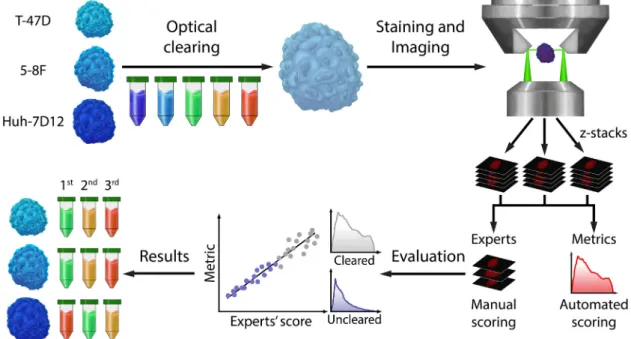
To evaluate the quality assessment metrics, we designed a 3D pipeline (Fig. 1). The seven metrics we consider here are commonly used to benchmark image sharpness in photos and videos, however, they characterize different aspects of the images. In order to vali- date these metrics, we first created a 3D dataset of cleared mono- culture spheroids (Fig. 2). All details are reported in[19]. Then, we asked ten microscopy experts (researchers that have been work- ing with spheroid images and possess at least 5 years of experience in microscopy) to visually evaluate the sharpness of the images and we correlated their evaluations with the results of the seven met- rics. Finally, to measure the efficacy of the clearing protocols, we used the metric that best correlated with the evaluation of the experts. In this article we report on our findings, organized as fol- lows: Section 2.2 (i.e. ‘‘Human evaluation”) summarizes the results of the human evaluation of the 3D dataset. InSection 2.3 (i.e.‘‘Quantitative metrics”) we discuss the results for image qual- ity assessment using the seven objective no-reference sharpness metrics that we implemented as an ImageJ/Fiji plugin. The correla- tion between the quality metrics and human evaluation, as well as the performance of the 5 optical clearing protocols tested are pre- sented inSection 2.4(i.e.‘‘Correlation and clearing results”).
2.2. Human evaluation
For a quantitative testing of the proposed metrics, a 3D light- sheet dataset of spheroids was used[19]. The dataset contained
Fig. 1.Representation of the 3D pipeline summarizing the concept of our experiments. Spheroids from T-47D, 5-8F, and Huh-7D12 cell lines with a similar size range (approx.
250mm) were cleared with ClearT, ClearT2, CUBIC, ScaleA2, and Sucrose protocols, and the nuclei of the cells were labeled with DRAQ5 staining. For imaging, a Leica SP8 digital light-sheet microscope was used, yieldingz-stack images. Ten experts evaluated the sharpness of the fluorescent images, and we compared their scoring with the tested quality metrics. Correlations between the quality metrics and human evaluation were calculated using Pearson’s correlation, and the metric with the best correlation was used to compare the efficacy of the optical clearing protocols applied on three types of spheroids originating from different cell lines.
fluorescence stack images of 90 spheroids that included three cell lines (T-47D, 5-8F, and Huh-7D12), five clearing protocols (ClearT, ClearT2, CUBIC, ScaleA2, and Sucrose), and an uncleared group as a control (the number of spheroids was n = 5 for each group).
Ten microscopy experts scored the LSFM images of the spheroids cleared with the optical clearing methods. The scores ranged from 1 to 5 (1 for the worst image quality and 5 for the sharpest image).
To assess the consistency of each expert’s evaluation, some of the images were repeated. On average, the self-accuracy of the ten experts reached 81.6% for the evaluation of repeated images. The best-case consistency was 92.1% and the worst-case one was 74.5%, and only four of the experts recognized the repeated images during the evaluation process. In general, the experts were more uncertain in case of the highest scores (i.e. ‘‘good” – 4 or ‘‘very good” – 5) were considered to be appropriate. Therefore, the scores for the T-47D and the 5-8F spheroids were less consistent com- pared to the Huh-7D12 spheroid. According to the experts, they could differentiate between the top, the middle and the bottom regions of the spheroids. The average results for the evaluation executed by the ten experts are represented on a heatmap (Fig. S1A). In general, the experts scored the T-47D spheroids higher, followed by the 5-8F spheroids, whereas the Huh-7D12 spheroids were characterized by the lowest scores. Comparing
the optical clearing protocols, the results for ClearT and ClearT2 were similar to the uncleared group, as the experts could hardly differentiate them from one another, however both of these clear- ing protocols decreased the size of the spheroids. Meanwhile, CUBIC, ScaleA2, and Sucrose protocols got higher scores for all the three regions of the spheroids, indicating that these optical clearings improved the transparency of the spheroids. We con- cluded that Sucrose was the only protocol that improved the image quality even at the bottom region for the Huh-7D12 spheroids, while the 5-8F and the T-47D spheroids had better scores when CUBIC and ScaleA2 protocols were applied. Both of these protocols reached very similar scores upon the experts’ evaluation, as no sig- nificant differences between these images could be detected by the human experts. Among the mentioned clearing protocols Sucrose resulted in minimal shrinkage, meanwhile CUBIC and ScaleA2 increased the volume of the spheroids. Regarding that currently there is no gold standard metric capable of assessing the differ- ences between the different protocols, we considered the results for the experts’ evaluation as ground truth to compare the metrics for their appropriateness to quantify the performance of the clear- ing protocols tested.
2.3. Quantitative metrics
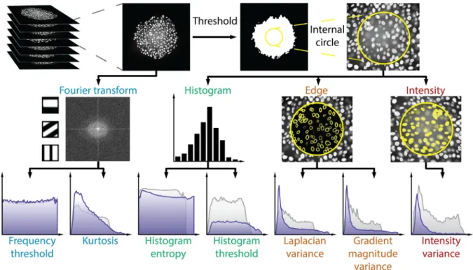
We implemented seven metrics in a user-friendly ImageJ/Fiji plugin to assess the quality of microscopy images, namely intensity variance, Laplacian variance, gradient magnitude variance, his- togram threshold, histogram entropy, kurtosis, and frequency threshold [24–28], and benchmarked them on 3D datasets. The metrics were applied on each optical section of the whole z- stacks independently, and the results were visualized. For his- togram, gradient, and intensity based metrics, we enabled the threshold option to obtain information from the area of the spher- oid. To handle the sharpness and contrast differences between the outer and inner layers of the spheroids, caused by the lateral light scattering effect, an internal circle option was also enabled which evaluates images inside the spheroids only. A schematic represen- tation of the metrics is shown inFig. 3, and an extended compar- ison of them is presented in Table 1. Detailed results for all the metrics evaluated on the Huh-7D12 cell line are shown inFig. S2.
2.3.1. Intensity variance
Intensity variance clearly differentiated the uncleared group from those that were cleared. The plot reaches the maximum vari- ance in the top region of the spheroid, and constantly decreases towards the deeper layers. Higher steepness of the plot indicates that visibility inside the spheroid is limited. In general, the uncleared spheroids lost intensity variance from top to the center, mainly in the first outer third, while the cleared and more trans- parent spheroids retained higher values through their whole thick- ness (Fig. 3andFig. S2). The results for the internal circle yielded plots of similar shape, but separated the cleared spheroids better.
This metric is one of the most basic methods, and it is a relatively fast approach for assessing image quality.
2.3.2. Derivative based metrics
Gradient magnitude variance and Laplacian variance metrics are also pixel based. Metrics that use image derivatives require pixel operations in order to yield a transformed image on which the final assessments are executed. These derivative metrics pro- vided plots similar to those yielded by the intensity variance method. Based on the evaluation of the whole spheroid, no differ- ences between these metrics were detected, however, the results for internal circle assessment separated the uncleared and cleared groups, and changed the order of the clearing protocols (Fig. 3and Fig. 2. 3D representation of the dataset. (A) 3D representation of a nuclei-labeled
Huh-7D12 spheroid cleared with Sucrose optical clearing protocol. For visualiza- tion, a square (110110300mm) from the middle part of the original spheroid was extracted. (B) For all the five clearing protocols, the same area was extracted from all the three cell lines. The scale bar represents 100mm. The images were taken and visualized with a LAS X microscope software developed by Leica.
Fig. S2). These findings suggest that the internal circle option is suitable to compare the optical clearing protocols.
2.3.3. Histogram based metrics
The histogram of a digital image shows the frequency of pixel intensities. Here we used two of the most popular histogram based methods for quality assessment, called histogram entropy and his- togram thresholding. Analysing the entire spheroids, histogram threshold reached the maximum values at the middle and it sepa- rated clearing groups from each other (Fig. S2). While, histogram entropy metric yielded consistent plots and the differences between the clearing groups were hardly visible. Based on the evaluation of the internal circle, the difference between the uncleared and cleared spheroids were remarkable when using his- togram thresholding metric, while histogram entropy plots showed the same consistent values across the spheroids. However, the assessment of the internal circle increased the differences and some of the cleared groups were separated from the uncleared group.
2.3.4. Frequency based metrics
To investigate the frequency space, frequency threshold and kurtosis were implemented in SQM and were evaluated on the whole image, without internal circle option. Frequency threshold metric failed to visualize the differences between the cleared and uncleared spheroids. Overall, frequency threshold yielded consis- tent plots, and the different optical clearing protocols were charac- terized by similar curves (Fig. 3andFig. S2). On the other hand, the kurtosis metric distinguished the cleared groups from one another, and the shapes of the curves were similar to those yielded by the intensity and derivative based metrics. This finding suggests that the frequency space can provide additional information about the images. However, performing all the necessary calculations to get
the bivariate kurtosis proved to be highly time consuming com- pared to the other metrics, and this drawback makes kurtosis less suitable for routine assessments.
2.4. Correlation and clearing results 2.4.1. Results of the metrics
According to the experts’ evaluation, the Uncleared, ClearTand ClearT2image groups were characterized by lower scores, while CUBIC, ScaleA2, and Sucrose got higher scores (Fig. S1A). Accord- ingly, we expected a gap between the well-performing and worse performing clearing protocols. Frequency threshold metric was unable to differentiate between the clearing protocols (Fig. S2).
Kurtosis metric, which can be calculated for the whole image only, yielded results similar to those obtained by intensity and edge based metrics, however, the slow processing time make this metric less effective. Histogram threshold metric distinguished between the optical clearing protocols, but the results did not match the ground truth: the ScaleA2 and the CUBIC protocols did not improve transparency compared to the uncleared group, which is in con- trast to the results for the experts’ evaluation. We also measured the histogram threshold metric in the internal circle of the spher- oids, where it showed greater differences between the cleared and uncleared groups, but the overall rank of the clearings was the same as for the whole spheroid. On the other hand, the histogram entropy metric, besides revealing differences among the clearing protocols, also matched the ground truth’s order of the protocols.
Furthermore, the assessment of the internal circle separated the clearing groups revealing greater differences between the proto- cols. Intensity variance, gradient magnitude variance, and Lapla- cian variance metrics yielded plots with very similar shape and almost the same order of the clearing protocols. Furthermore, intensity variance metric yielded similar results for the whole Fig. 3.Conceptual figure for the workflow of the quantitative metrics. The metrics based on Fourier transformation were evaluated on the whole image, whereas for the other metrics the automatic Otsu threshold was applied. For histogram, edge and intensity based metrics, the internal circle option was also enabled to assess the information content at the center of the objects only. The results for each metric were visualized as a plot describing sharpness across the spheroid, where the coordinate in thex-axis represents the number of the image within the stack, and they-axis is the score obtained by the metric. For histogram, edge and intensity based metrics, only the results for the internal circle are represented. Dark blue curves represent the uncleared spheroid, and gray curves represent the cleared spheroid. (For interpretation of the references to colour in this figure legend, the reader is referred to the web version of this article.)
spheroids and for the internal circle of the spheroids. Meanwhile, gradient magnitude and Laplacian metrics revealed greater differ- ences between the clearings, based on the internal circle assess- ments. Histogram entropy, histogram threshold, and frequency threshold methods yielded different line charts. Besides from the different line charts, all the metrics were reckoned to be worthy of further investigation to compare their correlation with the experts’ evaluation.
2.4.2. Correlation
To check if there is a quantitative metric able to reflect the experts’ evaluation, the Pearson’s correlation coefficient was com- puted between each metric and the ground truth by normalizing the results for all the spheroids. Here, we only discuss the intensity variance metric that showed the highest correlation with the experts either when applied to the whole spheroid or to the inter- nal circle only. This makes it an optimal candidate to assess quality differences. Considerations for the other metrics are reported in Supp. Note 1, with a detailed version of all the correlations and the individual normalization depicted inFig. S3.
The Pearson’s correlation coefficient for intensity variance resulted in 0.67 (Fig. 4A). The internal circle option improved the overall match with the experts’ evaluation and showed a higher correlation (0.80,Fig. 4A and E). The correlation between intensity variance and the experts’ scores was highest at the bottom regions of the spheroids and decreased at the middle and top regions. The Pearson’s correlation coefficient for the top, the middle, and the bottom regions were 0.46, 0.84, and 0.92 (Fig. 4B-D). Better image quality (like at the top region of the spheroids) and higher trans- parency of the spheroids weakened the correlations. This result might be contradictory, but it can be explained by the fact that the human decisions were less consistent with images of better quality because the experts found it difficult to decide the optimal score for them. In general, intensity variance metric showed the strongest correlation with the human scores in cases when the experts well distinguished the groups from one another (like at the bottom regions), independently of the type of the spheroids.
Moreover, a stronger correlation between intensity variance and the experts’ scores was revealed for the Huh-7D12 spheroids com- pared to the T-47D and 5-8F spheroids. We reckon that the fairly good overall 0.80 Pearson’s coefficient for the correlation between Table 1
Comparison of the metrics used in our experiments to quantitatively evaluate the imaging quality of spheroids. For the time comparison, 5 z-stacks with overall 295 images were processed using a consumer level laptop (Intel Core i5, CPU 1.80 GHz, 8 GB RAM).
Metric name Value(s) used Calculation of the metric
High value obtained Low value obtained
Advantages Drawbacks Computational
time (average) Intensity variance Grayscale pixel
values
Variance of intensity values
There are many different intensities in the image which are far away from one another in brightness
There is just one intensity value in the image
General usability, strongly associated with image sharpness, fast
Needs fine- tuning in specific cases
0.82 s/image
Gradient magnitude variance
Magnitude of the partial image derivative vectors
Variance of gradient magnitudes
There are many edges in the image with various magnitude values
There are no edges in the image, the image is homogeneous
Strongly associated with image sharpness, widely used in autofocus detection, fast
Very sensitive to noise, yields high values for blurred images with very sharp regions
0.86 s/image
Laplacian variance Second order image derivative values
Variance of the sum of second order derivatives
There are many edges in the image with various sharpness
There are no edges in the image, the image is homogeneous
Strongly associated with image sharpness, widely used in autofocus detection, fast
Noise sensitive, edges are not always indicative of image quality
0.92 s/image
Histogram thresholding
Image histogram values
Sum of histogram bin values above a predefined threshold (mean grayscale value), multiplied by their occurrence values
There are a lot of bright pixels in the image (theoretically when every pixel has the brightest value)
The pixels in the image have low brightness (theoretically when every pixel has 0 value)
Easy to calculate, fast
Applicable for image quality assessment in very specific cases only
0.88 s/image
Histogram entropy Image histogram values
Shannon entropy of the histogram as a vector of the occurrence values
Every histogram bin has the same value
Only 1 histogram bin has all the values
Strong theoretical background, used for image quality assessment, fast
Not closely related to image sharpness, histogram information might be misleading
0.94 s/image
Frequency thresholding
FFT magnitude image intensities
Sum of the intensities in the FFT image with a high-pass filter
Image contains a lot of high frequency components (edges, sharp noise)
Image is mostly made of low frequency components (homogeneous objects)
Edges can be detected very effectively in the FFT image, which is closely related to sharpness
Noise sensitive, threshold value is important
0.35 s/image
Kurtosis FFT magnitude
image of the autocorrelation image
Kurtosis of the periodogram as a bivariate probability distribution
There are less high frequency components on the FFT of the autocorrelation image
There are more high frequency components on the FFT of the autocorrelation image
Theory suits well to sharpness assessment
Very slow, less intuitive than some other metrics
2.78 s/image
intensity variance metric and the experts’ scores, indicates that intensity variance might be reliably used for the quality assess- ment of optical clearing protocols.
2.4.3. Clearing efficacy based on the intensity variance metric (based on internal circle assessment)
The correlation analysis confirmed that intensity variance met- ric yielded the highest scores both for the whole spheroid and for the internal circle assessments. Thus, in our further experiments we used this metric to visualize the spheroids treated by the five optical clearing protocols tested. Our primary aim was to find the best optical clearing protocol which is capable of clearing all the three types of spheroids in an appropriate manner. The metrics do not require a similar efficacy between the protocols to be compared. However, comparing clearing methods with a similar
efficacy it is easier. Regarding the methodology, it must be emphasized that the comparison of different clearing protocols presumes that every single protocol is applied on all different spheroid types, one by one, and the cleared spheroids are ana- lyzed by the chosen metric to reveal how each protocol performs on the different cell lines (Fig. 5A). In contrast, when different clearing protocols are applied in parallel on a well-defined spher- oid type, the results can only show the best protocol for the cell line of interest, but this type of experiment is inappropriate for the evaluation of the relative efficacy of the different clearing pro- tocols on various spheroid types (Fig. 5B). This methodological issue is explained by the fact that different normalization scales are used for the assessment of each sample type (Fig. 5 and Fig. S4). All three types of spheroids were treated with each clear- ing protocol, and were analyzed using intensity variance metric, Fig. 4.Correlation between the metrics and the experts’ evaluation. (A) Results for the Pearson’s correlation analysis between the metrics and the experts’ assessment.
Metrics were evaluated considering all the cell lines together. Bounding boxes with dashed lines represent the results of the internal circle assessment. (B-D) Correlation results for the three regions of the spheroids. (E) For a reliable calculation of the correlation between a metric and the experts’ assessment (i.e. the ground truth), all three regions of spheroids were included. Dark-blue dots represent the Huh-7D12 spheroids; blue dots the 5-8F spheroids; light-blue dots the T-47D spheroids. The correlation was visualized with linear regression, and the Pearson’s correlation coefficient was calculated for all the spheroids. In total, 54 pairs were tested to assess the overall correlation between the metrics and expert assessment, whereas only 18 pairs were tested to demonstrate the correlations at the different regions. (For interpretation of the references to colour in this figure legend, the reader is referred to the web version of this article.)
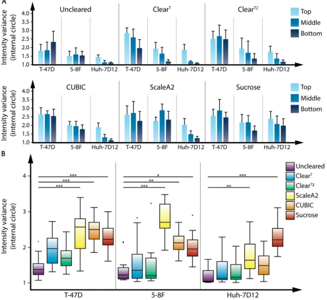
separated to top, middle and bottom regions. Using intensity vari- ance, the T-47D spheroid reached the highest scores, followed by 5-8F and Huh-7D12, which confirmed the transparency differ- ences among the spheroids derived from various cell lines. In all cases, the top and the middle regions of the spheroids reached higher scores than the bottom, which also confirms the presence of vertical light scattering. The results for internal circle assess- ments differed from the results related to the whole spheroid.
Regarding the efficacy of the optical clearing protocols, the analy- sis revealed that Sucrose increased transparency for all the spher- oids (Fig. 5A), but the total score for the three spheroid types were not similar in all the regions. The efficacy of the clearing protocols revealed that ScaleA2 and CUBIC clearing protocols were success- ful on certain cell lines only, but not on all the three types of spheroids (Fig. 5B). When the cleared groups were compared to the control group, we noticed that ClearTand ClearT2 increased transparency especially at the top region of the spheroids.
Although they both slightly improved the scores, the results did
not differ significantly from the scoring of the uncleared spheroids (Fig. 5A and B). In case of the T-47D spheroids, CUBIC, ScaleA2, and Sucrose protocols improved transparency significantly, but the differences among these groups were minimal. In case of the 5-8F spheroids, ScaleA2 protocol significantly improved image quality, yielding high quality images with low background signals.
For the Huh-7D12 spheroids, Sucrose reached the highest scores (Fig. 5B). In general, the scores for the whole spheroid assess- ments were higher than those for the internal circle assessments, because the outer parts of the spheroids improved the values (Fig. S4). Due to the lateral illumination by the light-sheet micro- scope, the higher contrast of the nuclei at the outer shell reduced the accuracy of the comparison, leading to modified overall results. Based on the whole spheroid assessments, all clearing protocols improved the overall scores for each cell line. The differ- ences among CUBIC, ScaleA2 and Sucrose clearing protocols decreased, but the order of the protocols slightly changed in case of the 5-8F and Huh-7D12 spheroids (Fig. S4B).
Fig. 5.Results for the clearing protocols (A) Performance (efficacy) of the clearing protocols on the spheroid types derived from different cell lines. Three types of spheroids were compared at three regions (top, middle, bottom) using intensity variance metric with the internal circle option, after applying each clearing protocol. The scores represent the results for the different types of spheroids treated with the same clearing protocol. (B) Comparison of the clearing protocols on each spheroid type to reveal the most appropriate method for each cell line. Intensity variance was used with the internal circle option to assess the quality of each protocol. The efficacy of each clearing protocol was compared to the uncleared spheroids of the same type. Each cleared group contains five spheroids that were divided into three regions (top, middle and bottom), yielding 15 values per group for quality assessment. *p0.05; **p0.01; ***p0.001.
3. Discussion
Regarding microscopy image analysis of 3Din vitromodels, the quality of the acquired images depends on the size, shape and incu- bation time and cell line composing the 3D model. These features and conditions often lead to inconsistency in the acquired images’
quality. The efficacy of optical clearing protocols applied to enhance image quality highly depends on the cell line. Thus, choosing the best optical clearing protocol for the target 3D model is crucial. Cur- rently, plenty of different approaches are utilized to assess the effi- ciency of clearing protocols for 3D samples. However, there is no gold standard metric to quantitatively evaluate and compare the different clearing protocols. In most studies of newly developed clearing protocols both qualitative and quantitative approaches were used to assess clearing efficacy. Among the qualitative approaches, most of the researchers simply used subjective scoring, based on microscopy images before and after optical clearing. These experiments are based on the ratings of brightfield and fluorescence microscopy images[29]. In fact, this method is appropriate when we simply have to decide whether fluorescent signals are present or absent after the clearing process, or when we simply need to dis- tinguish different clearing protocols based on brightfield images.
However, these measurements are time-consuming, and are not feasible when hundreds of 3D images are to be compared.
Some of the qualitative metrics aim to assess the changes in various fluorescence intensity profiles: intensity/contrast increases in both lateral and axial dimensions; tissue transparency improves due to clearing. The basic concept of this approach is the signal-to- background (SNB) ratio, which is defined as the ratio between the mean signal and the standard deviation of the background signal in the intensity profile. To obtain this ratio, an intensity threshold is usually applied to determine background (values below threshold) and signal intensities (values above threshold) [30]. As another option, calculating the changes in mean fluorescence intensity at different imaging depths of a 3D sample can also be used to assess lateral or axial imaging depth[31,32]. Furthermore, corrected total cell fluorescence (CTCF) was also introduced to monitor the loss of the fluorescent signal in response to optical clearing [31–34]. A recent study has developed an improved signal-to-noise ratio (SNR) based method to characterize depth-dependent signal inten- sity [35]. Regarding the well-established correlation between image quality improvement and fluorescence intensity changes, assessing these alterations is quite a popular approach in literature.
However, as a disadvantage of intensity values, the results are highly sensitive to staining quality and imaging settings, such as exposure time. Furthermore, the results of these analyses are highly dependent on the applied threshold as well, which might easily lead to the misinterpretation of total intensity changes for a whole spheroid.
A different approach to assess the performance of an optical clearing protocol is based on the concept that the number of well-segmented nuclei should be increased within the entire spheroid as image quality improves[36]. An obvious drawback of using the segmentation-based approach (to compare the efficacy of various clearing protocols) is that the results are highly depen- dent on the precision of the applied segmentation approach.
Based on these considerations, instead of using only the inten- sity values of the images or the information for the segmented nuclei, we tested seven metrics which are used to characterize blurriness of general photos and videos. Implemented in a user- friendly ImageJ/Fiji plugin, the seven metrics were tested on a large public available 3D dataset[19], quantifying the quality of micro- scopy images of different spheroid types. The results for these metrics-based analyses were compared to the sharpness ratings of the images executed by ten human experts, and the correlation
between the two approaches was assessed. Among the seven met- rics tested, intensity variance obtained the highest correlation with the experts’ evaluation. In this case, the results for the whole spheroid and for the internal circle showed relatively strong corre- lations with ground truth. Comparing the results for the different regions (top, middle, bottom) of the spheroid, we found that this metric strongly correlated with ground truth at the bottom and middle regions, while the correlation was only acceptable in the top region. The correlation between intensity variance metric and the human scores was the strongest in those cases when the experts could consistently differentiate the groups from one another, like in case of images of the bottom and middle regions.
Meanwhile, for images of similar quality, such as images of the T-47D and 5-8F spheroids or images of the top regions, the experts could not distinguish the different clearings protocols. Since, the experts’ evaluation was the least consistent with the T-47D and 5-8F spheroids, we have concluded that even the best metric may not definitely show a really strong correlation with human assessment in these cases. However, an overall good correlation (Pearson 0.80) between the metrics and the experts suggests that intensity variance metric in point may serve as a quantitative tool to evaluate the relative efficacy of optical clearing protocols. Our results indicated that the appropriate protocol for optical clearing strongly depends on the cell line composing the spheroid. Further- more, by comparing the results for the whole spheroid and for the internal part separately, we were able to measure the lateral light scattering effect. This effect is common with light-sheet micro- scopy systems where the samples are illuminated from the side resulting in great differences between the outer region and the internal parts of the spheroid. The results for the internal circle showed higher correlation with the experts’ evaluation, suggesting that image analysis data related to the internal part of the spheroid could be applicable in practice.
As expected, none of the tested optical clearing protocols per- formed equally well on all three cell lines. In case of the T-47D cell line, which forms the least compact spheroids, Sucrose, CUBIC and ScaleA2 protocols proved to be equally effective, yielding no signif- icant quality differences among the cleared groups. The 5-8F spheroids showed the best image quality with the ScaleA2 clearing protocol. Finally, regarding the Huh-7D12, only Sucrose clearing protocol was able to visualise single nuclei located at the bottom regions of the spheroids. We also tested the reversible ClearTand ClearT2 protocols and found that in case of the ClearT protocol image analysis improved after the spheroids were washed, which suggests that this clearing method is in fact not completely rever- sible. Also, we could measure the differences between ClearTand ClearT2precisely, which provides a practical benefit to distinguish between slightly different clearings. Specifically, as these two pro- tocols differ in a single component only, the effects of a protocol’s composition on spheroid transparency can also be evaluated based on image analysis.
In summary, we introduced seven metrics for image quality assessment, implemented in SQM, a user-friendly open-source ImageJ/Fiji plugin. We aimed to find a metric suitable for the quan- titative assessment ofz-stack images of 3D spheroids, allowing to compare optical clearing protocols without pre-processing of images. We tested the correlation between the metrics and the human experts’ evaluation (regarded as the ground truth), and found that of the seven implemented metrics, only intensity vari- ance showed a good correlation, at least in the bottom and middle regions, with the experts’ assessment. This metric is suitable to quantitatively compare different optical clearing protocols and spheroids derived from various human carcinoma cell lines. Based on these findings, we support intensity variance as the gold stan- dard metric to quantitatively compare optical clearing protocols.
4. Materials and methods
4.1. Intensity variance
For the intensity metric[25]the average and variance are calcu- lated with the following formulas:
Iaverage¼ 1 MN
XN i¼1
XM
j¼1Iði;jÞ; ð1Þ
Var¼ 1 MN
XN i¼1
XM
j¼1I i;ð Þ j Iaverage2
; ð2Þ
whereIis the image with a resolution ofMN. Images with high variance indicate that there are pixels from very dark to bright val- ues, which may suggest that the image is not blurred.
4.2. Derivative based metrics
Image gradient calculation is based on the differentiation of multivariable functions[25]: the partial derivatives of the image function I xð;yÞrI xð;yÞ ¼ @x@I;@y@IT
represent the sharpness of the horizontal and vertical edges in the original image. This can be visualized by the magnitude of the gradients (jrIðx;yÞj ¼ ffiffiffiffiffiffiffiffiffiffiffiffiffiffiffiffiffiffiffiffiffiffiffiffiffi
ð@x@IÞ2þ ð@y@IÞ2 q
). After that, the mean and the variance of the gradient image can be calculated. Our implementation con- tains the variance of the gradient magnitude values:
G¼ 1 MN
XN i¼1
XM
j¼1jrI i;ð Þj jj rIjaverage2
; ð3Þ
where jrIjaverage¼ 1
MN XN
i¼1
XM
j¼1jrIði;jÞj: ð4Þ
Second order derivatives can also be used for focus detection, for example with the Laplacian operator[26]. The Laplacian of an image can be calculated with the following formula:
Lðx;yÞ ¼@2I
@x2þ@2I
@y2: ð5Þ
Next, we calculate the variance of the Laplacian the same way as we did for the gradient magnitudes.
4.3. Histogram based metrics
The approach defines a threshold valueT, and sums brightness values above that threshold, weighted by the number of pixels with that particular intensity.T is usually chosen as the average intensity in the image. Histogram threshold[27]metric is calcu- lated with the following equation:
Mhist¼X
ijxi>TxifðxiÞ; ð6Þ
wherexiare the pixel intensities andf is the histogram function.
Another histogram metric can be calculated using entropy[27], which is more precise for image quality assessment. The entropy is higher when the intensities are less predictable, i.e. they are more varied and not homogeneous. It is calculated as follows:
Ment¼ X
i
f xð Þi
Hmax
log2f xð Þi
Hmax
; ð7Þ
whereHmaxis the vertical maximum of the histogram.
4.4. Frequency based metrics
Frequency based metrics rely on the 2 dimensional Fourier transformation, which converts an image from its original space to frequency space. It breaks down the image to a sum of weighted sine and cosine waves. Each pixel intensity at a positionðu;
v
Þrep-resents the amplitude of the function with a certain frequency component characterized byu and
v
: Around the center of the resulting image lower frequency components are found, so a high amplitude in the middle corresponds to a homogeneous territory in the original image. With a growing distance from the center alongside concentric circles, higher frequency components are found. High amplitudes at the sides of the Fourier image usually correspond to sharp edges or noise in the original image.The discrete Fourier transformation of an image can be formal- ized as follows:
F u;ð
v
Þ ¼X1m¼1X1n¼1Iðm;nÞe2piðumþvnÞ: ð8ÞThe calculated function F uð ;
v
Þ is a complex function, so for visualization,jF uð ;v
Þjis typically used:F u;ð
v
Þj j ¼
ffiffiffiffiffiffiffiffiffiffiffiffiffiffiffiffiffiffiffiffiffiffiffiffiffiffiffiffiffiffiffiffiffiffiffiffiffiffiffiffiffiffiffiffiffiffiffiffiffiffiffiffiffiffiffiffiffi Re F u;ð ð
v
ÞÞ2þIm F u;ð ðv
ÞÞ2q
; ð9Þ
whereReðzÞandImðzÞare the real and imaginary parts of a complex numberz.
One metric that can be calculated in the Fourier space is the fre- quency threshold metric[25]. Exactly how to measure sharpness in this domain varies. In this study, we defined a frequency threshold, and summed the amplitude values above that value only. This means that we sum the pixel values in the Fourier space outside a circle mask with radius r. Applying the mask is equivalent to multiplying the Fourier transformed image by a high-pass filter:
mask1:¼ fð Þjji;j 2þi2>r2g;
Mfreq¼X
i;j
ð Þ2mask1jF i;ð Þjj: ð10Þ
Kurtosis was proposed as an image sharpness measure[28]. The frequency space is utilized here as well, however, instead of using the Fourier magnitude image, kurtosis metric is calculated on the periodogram of the image, which is the Fourier transform of the autocorrelation image. The periodogram can be calculated as A u;ð
v
Þ ¼ jF u;ðv
Þ F u;ðv
Þj ð11ÞwhereF uð ;
v
Þis the complex conjugate ofF uð ;v
Þ. To calculate the kurtosis of the periodogram, it is beneficial to regard it as a proba- bility distribution. This can be achieved by normalization. We denote the frequencies at certain points of the periodogram by ui;v
jði¼1;2; ;NÞ, and calculate the normalized image with h u i;v
j¼P A u i;v
jn
P
mA uð n;
v
mÞ ð12Þfor everyi;j¼1;2; ;N.
The bivariate kurtosis of our probability distribution is calcu- lated as
b2;2¼
c
4;0þc
0;4þ2c
2;2þ4q
12ðq
12c
2;2c
1;3c
3;1Þ 1q
2122 ; ð13Þ
where
c
k;l¼ PNi¼1
PN
j¼1hðui;
v
jÞðuil
uÞkðv
jl
vÞlr
kur
lv ; ð14Þand
q
12is the normalized correlation betweenuandv
(q
12¼rruvurv).
The marginal means and variances ofh uð ;
v
Þarel
u¼XN i¼1uiXN
j¼1hðui;
v
jÞ;l
v¼XNj¼1v
jXNi¼1hðui;v
jÞ; ð15Þand
r
2u¼XNi¼1ðui
l
uÞ2XNj¼1hðui;
v
jÞ;r
2v¼XN
j¼1ð
v
jl
vÞ2XNi¼1hðui;v
jÞ: ð16ÞContrary to other metrics, a low number for kurtosis indicates a well-focused image, whereas high metric values suggest that the measured image is blurry.
4.5. Variance of normalized values inside the spheroid
We posed some conditions for the assessments of the fluores- cence images:
1. In an image of a spheroid, our volume of interest is the spheroid itself only, the background contains no relevant information, so we do not want to use it.
2. Intensity values highly depend on the quality of the staining and image acquisition. Metrics can behave differently for higher and lower intensity ranges, therefore, normalization is necessary.
3. Certain clearing agents are not appropriate to penetrate into the spheroids, as a result the edges become very sharp, while the internal part remains blurred. For most of the metrics, this can result in an overall high contrast value due to the very sharp edges on the side, which may lead to misinterpretation. There- fore, we assess both the whole spheroid and the internal part of the spheroid, and compare the results.
To satisfy the 1st criterium, we applied a threshold to the spher- oids, which can easily be achieved by the Otsu threshold algo- rithm: the spheroid area is very well distinguishable from the background based on the image histogram.
For intensity normalization (2nd criterium), we took the maxi- mum intensity value of the 3D image stack and divided every pixel value with that.
To assess the internal part of the spheroid separately (3rd cri- terium), we calculated the center of the spheroid mass, slice by slice, using image moments:
ðcenterx;centeryÞ ¼ M1;0 M0;0;M0;1
M0;0
;
where Mi;j¼X
x
X
yxiyjI x;ð yÞ: ð17Þ
We then calculated a desired pixel-based metric inside a circle with a radius ofrand with the center calculated above:
mask2:¼ fð Þji;j ðjcenterxÞ2þ icentery
2
<r2g:
Our internal circle results were obtained with a 200 pixel radius circle. The usage of this is optional, and the radius can be changed.
The choice of 200 pixel radius (~55mm diameter) was to measure a large enough area (~10 nuclei at minimum) to have stable analysis but small enough to have reasonable coverage at the top and bot- tom of the spheroids.
4.6. Score calculation
We have introduced a metric which can be calculated after plot- ting the slice-by-slice metric plots. These steps were necessary to make the metrics comparable with the results of the expert evalu- ations. Let there bekdifferent spheroid assessments, and letgibe
the calculated metric plot for the i-th spheroid in the domain f1; ;ng, wherendenotes the number of slices in the image stack, and let
a
be the maximum, andbbe the minimum value from all the assessedgiplots:a
¼maxgið Þ;xb¼mingið Þ;x i¼1; ;k:
We define our single-value score for every assessment with:
scorei¼ 1 ð
a
bÞnXn
j¼1ðgiðjÞ bÞ ð18Þ
With this number, ranging between 0 and 1, the quality of spheroid images relative to one another can be characterized in a given assessment set. The theoretical maximum (1) is a perfect rectangle with a height of
a
b, which would mean that an image with such a metric plot maintains the highest metric assessment across all of its slices. The theoretical minimum (0) is the constant zero function, which would mean that an image with such a metric plot gets a score of 0 for all of its slices. If an image maintains high metric values for most of the slices, its score will be closer to 1, whereas those images that consistently give low metric values, or the ones that have high values at the beginning, but then dras- tically decrease, will be closer to 0. In order to scale these scores to the human scoring system, we normalized all resulting values between 1 and 5. For all the metrics, the plots were divided into three equal regions, and the score calculation method described above was used. These steps do not change the results of the met- rics, just scale them to match with the scoring system of the experts. For all five clearing protocol groups, as well as for the con- trol group, the top, the middle, and the bottom regions of the spheroids were evaluated. Ten experts evaluated five spheroids from each clearing protocol group, but only one image from each region. The average of their scores was compared with the metrics.The results of the metrics were calculated almost the same way, except that the metrics evaluated all the images from each region, and the average scores were used for comparison. The whole spheroid and the internal circle were evaluated the same way, and the results were also calculated the same way. Next, the experts’ evaluation and the metrics’ scores were matched, and a linear regression analysis was carried out. For comparison, Pear- son’s correlation was used.
All the metrics were implemented in a user-friendly open- source ImageJ/Fiji[17,18]plugin named SQM. The results for score calculation are available as a csv file, saved by the plugin at the end of each image analysis process. SQM is implemented in Java and it works under Macintosh, Linux, and Windows 64-bit systems.
There are no special hardware requirements. SQM can be down- loaded from the Fiji plugin store, but it is also available at:
https://bitbucket.org/biomag/qualitymetricplugin/downloads/
4.7. Statistical analyses
Statistical analyses were performed using the R software. The Kolmogorov-Smirnov test was utilized to check for normal distri- bution. For the statistical analysis of the optical clearing results, non-parametric Kruskal-Wallis test with Dunn’s multiple compar- isons was performed. Significance level was set to
a
= 0.05 with a 95% confidence interval, andp-values were adjusted to account for multiple comparisons.Author contributions
A.D., D.H., M.K., K.K., and P.H. conceived the project. A.D., D.H., M.K., T.T., and M.H. designed and performed the experiments.
A.D., D.H., M.K., T.T., M.H., F.P., and P.H. analysed the data. A.D., D.
H., and K.K. designed the software. A.D., D.H., M.K., T.T., and F.P.
wrote the manuscript. M.H., K.K., K.B., and P.H. reviewed the manu- script. K.B., F.P., and P.H. supervised the project. All authors dis- cussed the conclusions and commented on the manuscript. All authors read and approved the final version of the manuscript.
Data and materials availability
All data needed to evaluate the conclusions in the paper are pre- sent in this paper, the Data in Brief article, and/or the Supplemen- tary Materials. Additional data related to this paper may be requested from the authors. The 3D dataset is available in FigShare at: https://doi.org/10.6084/m9.figshare.c.5051999.v1. SQM is available in BitBucket at: https://bitbucket.org/biomag/quality- metricplugin/downloads/.
Declaration of Competing Interest
The authors declare that they have no known competing finan- cial interests or personal relationships that could have appeared to influence the work reported in this paper.
Acknowledgments
The authors would like to thank Dr. Ji Ming Wang (National Cancer Institute-Frederick, Frederick, MD, USA) for kindly provid- ing us with the 5-8F cell line; Francesco Pampaloni (Goethe University, Frankfurt, Germany) for providing spheroid screening sample holders; Dora Bokor, PharmD (BRC, Szeged, Hungary) for proofreading the manuscript. Funding: A.D., D.H., M.K., T.T., M.H., K.K., B.K., and P.H. acknowledge support from the LENDULET- BIOMAG Grant (2018-342), from the European Regional Develop- ment Funds (GINOP-2.3.2-15-2016-00006, GINOP-2.3.2-15-2016- 00026, GINOP-2.3.2-15-2016-00037), from the H2020-discovAIR (874656), from the H2020 ATTRACT-SpheroidPicker, and from Chan Zuckerberg Initiative, Seed Networks for the HCA-DVP. FP acknowledges support from the Union for International Cancer Control (UICC) for a UICC Yamagiwa-Yoshida (YY) Memorial Inter- national Cancer Study Grant (ref: UICC-YY/678329).
Appendix A. Supplementary data
Supplementary data to this article can be found online at https://doi.org/10.1016/j.csbj.2021.01.040.
References
[1] Hoarau-Véchot J, Rafii A, Touboul C, Pasquier J. Halfway between 2D and animal models: are 3D cultures the ideal tool to study cancer- microenvironment interactions?. Int J Mol Sci 2018;19. https://doi.org/
10.3390/ijms19010181.
[2] Carragher N, Piccinini F, Tesei A, Jr OJT, Bickle M, Horvath P. Concerns, challenges and promises of high-content analysis of 3D cellular models. Nature Rev Drug Discov 2018;17:606.https://doi.org/10.1038/nrd.2018.99.
[3]Piccinini F, De Santis I, Bevilacqua A. Advances in cancer modeling: fluidic systems for increasing representativeness of large 3D multicellular spheroids.
Biotechniques 2018;65:312–4.
[4] Cesarz Z, Tamama K. Spheroid culture of mesenchymal stem cells. Stem Cells Int 2016;2016:1–11.https://doi.org/10.1155/2016/9176357 (2016).
[5]Sawant-Basak A, Obach RS. Emerging models of drug metabolism, transporters, and toxicity. Drug Metab Dispos 2018;46:1556–61.
[6]Sant S, Johnston PA. The production of 3D tumor spheroids for cancer drug discovery. Drug Discov Today: Technol 2017;23:27–36.
[7]Di Modugno F, Colosi C, Trono P, Antonacci G, Ruocco G, Nisticò P. 3D models in the new era of immune oncology: focus on T cells, CAF and ECM. J Exp Clin Cancer Res 2019;38:1–14.
[8]Swinney DC, Anthony J. How were new medicines discovered?. Nat Rev Drug Discov 2011;10:507–19.
[9]Smith K, Piccinini F, Balassa T, Koos K, Danka T, Azizpour H, et al. Phenotypic image analysis software tools for exploring and understanding big image data from cell-based assays. Cell Syst 2018;6:636–53.
[10] Method of the Year 2014. Nature methods. 12, 1 (2015).
[11]Power RM, Huisken J. A guide to light-sheet fluorescence microscopy for multiscale imaging. Nat Methods 2017;14:360–73.
[12]Zanoni M, Piccinini F, Arienti C, Zamagni A, Santi S, Polico R, et al. 3D tumor spheroid models for in vitro therapeutic screening: a systematic approach to enhance the biological relevance of data obtained. Sci Rep 2016;6:1–11.
[13]Costa EC, Silva DN, Moreira AF, Correia IJ. Optical clearing methods: an overview of the techniques used for the imaging of 3D spheroids. Biotechnol Bioeng 2019;116:2742–63.
[14]Richardson DS, Lichtman JW. Clarifying tissue clearing. Cell 2015;162.
[15]Tainaka K, Kuno A, Kubota SI, Murakami T, Ueda HR. Chemical principles in tissue clearing and staining protocols for whole-body cell profiling. Annu Rev Cell Dev Biol 2016;32.
[16]Dekkers JF, Alieva M, Wellens LM, Ariese HCR, Jamieson PR, Vonk AM, et al.
High-resolution 3D imaging of fixed and cleared organoids. Nat Protoc 2019;14:1756–71.
[17]Abràmoff MD, Magalhães PJ, Ram SJ. Image processing with imageJ. Biophoton Int 2004;11:36–41.
[18] Schindelin J, Arganda-Carrera I, Frise E, Verena K, Mark L, Tobias P, et al. Fiji - an open platform for biological image analysis. Nat Methods 2009;9.https://
doi.org/10.1038/nmeth.2019.Fiji.
[19] Diosdi A, Hirling D, Kovacs M, Toth T, Harmati M, Koos K, Buzas K, Piccinini F, Horvath P. Cell lines and clearing approaches: a single-cell level 3D light-sheet fluorescence microscopy dataset of multicellular spheroids. Data in Brief 2021;107090.https://doi.org/10.1016/j.dib.2021.107090.
[20]Kuwajima T, Sitko AA, Bhansali P, Jurgens C, Guido W, Mason C. ClearT: a detergent- and solvent-free clearing method for neuronal and non-neuronal tissue. Development 2013;140:1364–8.
[21]Susaki EA, Tainaka K, Perrin D, Kishino F, Tawara T, Watanabe TM, et al.
Whole-brain imaging with single-cell resolution using chemical cocktails and computational analysis. Cell 2014;157:726–39.
[22]Hama H, Kurokawa H, Kawano H, Ando R, Shimogori T, Noda H, et al. Scale: a chemical approach for fluorescence imaging and reconstruction of transparent mouse brain. Nat Neurosci 2011;14:1481–8.
[23]Tsai PS, Kaufhold JP, Blinder P, Friedman B, Drew PJ, Karten HJ, Lyden PD, Kleinfeld D. Correlations of neuronal and microvascular densities in murine cortex revealed by direct counting and colocalization of nuclei and vessels. J Neurosci 2009;29(46):14553–70.
[24]Ferzli R, Karam LJ. A no-reference objective image sharpness metric based on just-noticeable blur and probability summation. Proc - Int Conf Image Process, ICIP 2006;3:445–8.
[25]Batten CF. Autofocusing and astigmatism correction in the Scanning Electron Microscope. University of Cambridge; 2000.
[26]Pech-Pacheco J, Cristobal JL, Chamorro-Martinez G, Fernandez-Valdivia J.
Diatom autofocusing in brightfield microscopy: a comparative study. In: 15th International Conference on Pattern Recognition. p. 314–7.
[27]Firestone L, Cook K, Culp K, Talsania N, Preston K. Comparison of autofocus methods for automated microscopy. Cytometry 1991;12:195–206.
[28]Zhang N, Vladar A, Postek M, Larrabee B. A kurtosis-based statistical measure for two-dimensional processes and its application to image sharpness. Proc Sect Phys Eng Sci Am Statist Soc 2003;4730–4736.
[29]Kolesová H, Cˇapek M, Radochová B, Janácˇek J, Sedmera D. Comparison of different tissue clearing methods and 3D imaging techniques for visualization of GFP-expressing mouse embryos and embryonic hearts. Histochem Cell Biol 2016;146:141–52.
[30]Smyrek I, Stelzer EHK. Quantitative three-dimensional evaluation of immunofluorescence staining for large whole mount spheroids with light sheet microscopy. Biomed Opt Express 2017;8:484.
[31]Costa EC, Moreira AF, De Melo-diogo D, Correia IJ. Polyethylene glycol molecular weight influences the ClearT2 optical clearing method for spheroids imaging by confocal laser scanning microscopy. J Biomed Opt 2018;23:1.
[32]Costa EC, Moreira AF, de Melo-Diogo D, Correia IJ. ClearT immersion optical clearing method for intact 3D spheroids imaging through confocal laser scanning microscopy. Opt Laser Technol 2018;106:94–9.
[33] Ansari N, Müller S, Stelzer EHK, Pampaloni F. In: Quantitative 3D cell-based assay performed with cellular spheroids and fluorescence microscopy. Elsevier; 2013. https://doi.org/10.1016/B978-0-12-407239- 8.00013-6.
[34]Klaka P, Grüdl S, Banowski B, Giesen M, Sättler A, Proksch P, et al. A novel organotypic 3D sweat gland model with physiological functionality. PLoS One 2017;12:1–18.
[35]Nürnberg E, Vitacolonna M, Klicks J, von Molitor E, Cesetti T, Keller F, et al.
Routine optical clearing of 3D-cell cultures: simplicity forward. Front Mol Biosci 2020;7:1–19.
[36]Boutin ME, Voss TC, Titus SA, Cruz-Gutierrez K, Michael S, Ferrer M. A high- throughput imaging and nuclear segmentation analysis protocol for cleared 3D culture models. Sci Rep 2018;8:1–14.